Predictable properties of fitness landscapes induced by adaptational tradeoffs
- Institute for Biological Physics, University of Cologne, Germany
- School of Physics and Astronomy, University of Edinburgh, United Kingdom
Figures
Figure 1
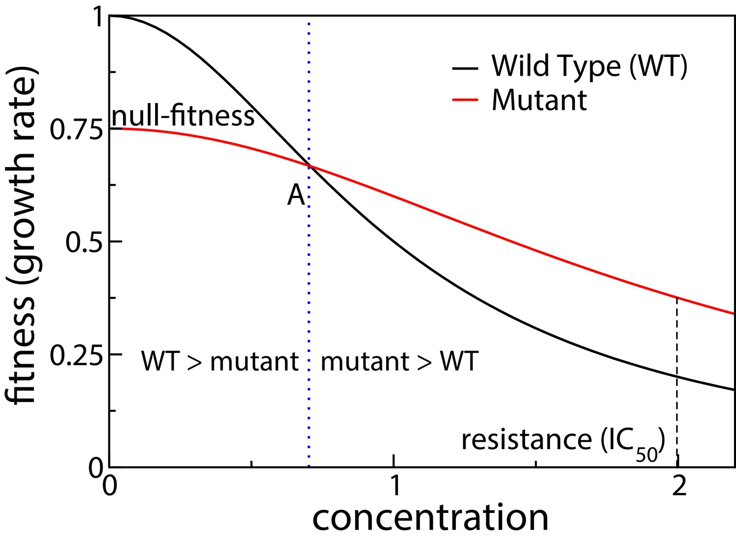
Schematic showing dose response curves of a wild type and a mutant.
To the left of the intersection point A the wild type is selected over the mutant, whereas to the right of A the mutant is selected.
Figure 2
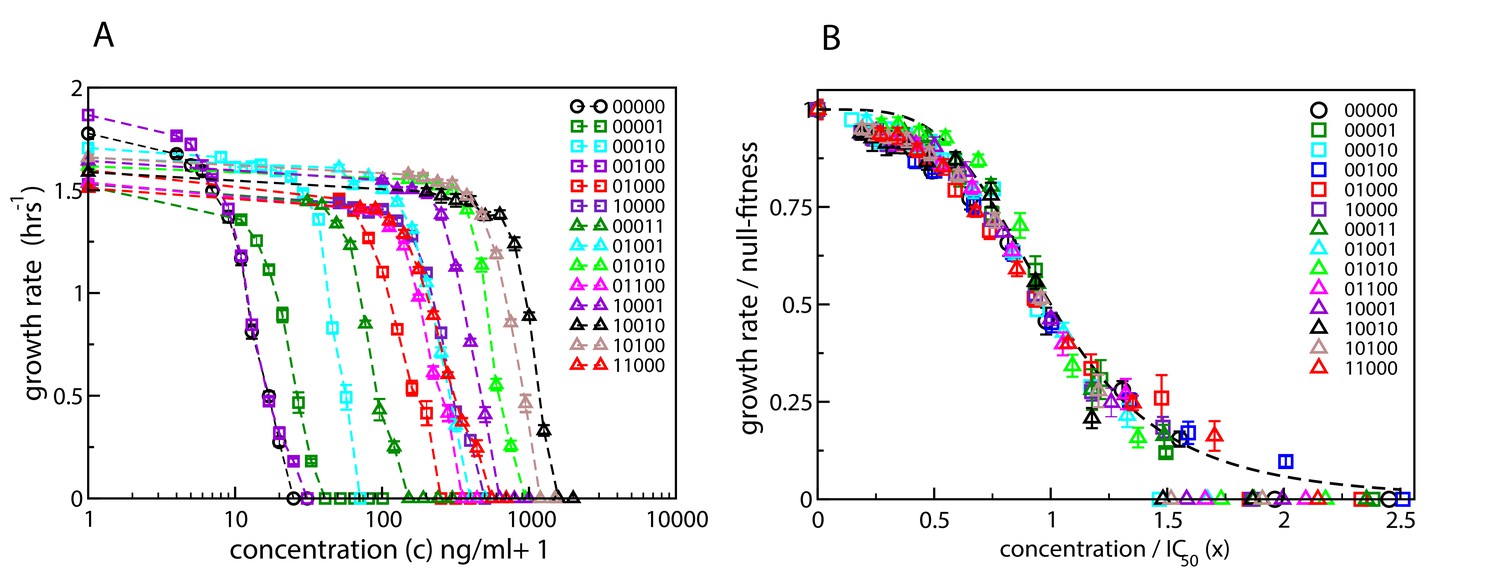
Dose-response curves for E. coli in the presence of ciprofloxacin.
Each binary string corresponds to a strain, where the presence (absence) of a specific mutation in the strain is indicated by a 1 (0). The five mutations in order from left to right are S83L (gyrA), D87N (gyrA), S80I (parC), marR, and acrR. The names of the strains are given in Table 1. (A) Dose-response curves of the wild type, the five single mutants and eight double mutants. Unlike the experiments reported in Marcusson et al., 2009, the mutants were grown in isolation rather than in competition with the wild type. (B) The same curves, but scaled with the null-fitness and IC50 of each individual genotype. The dashed black line is the Hill function .
Figure 3
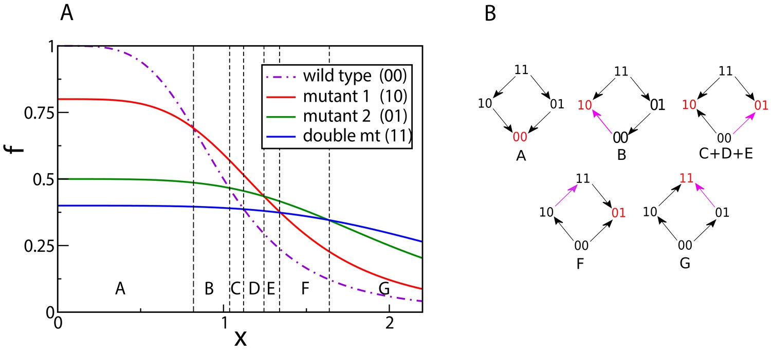
Crossing dose-response curves and fitness graphs.
(A) An example of dose-response curves of four genotypes – the wild type (00), two single mutants (10 and 01), and the double mutant (11). The parameters of the two single mutants are , , , . Null-fitness and resistance combine multiplicatively, which implies that the parameters of the double mutant are and . (B) Fitness graphs corresponding to antibiotic concentration ranges from panel (A). The genotypes in red are the local fitness peaks. The purple arrows are the ones that have changed direction at the beginning of each segment. All arrows eventually switch from the downward to the upward direction.
Figure 4
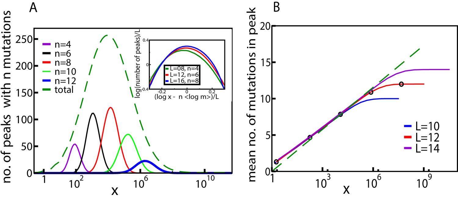
Fitness landscape ruggedness changes with drug concentration.
(A) Number of fitness peaks as a function of concentration for different numbers of mutations in the peak, , and . The dashed green curve is the total number of fitness peaks, summed over . The peaks were found by numerically generating an ensemble of landscapes with individual effects distributed according to the joint distribution (8). For this distribution, . Inset: The maximal number of peaks for a given value of occurs at , and grows exponentially with . (B) Mean number of mutations in a fitness peak as a function of concentration for the same model. The black circles are the mean number of mutations in the fittest genotype. The green dashed line is , where as before.
Figure 5
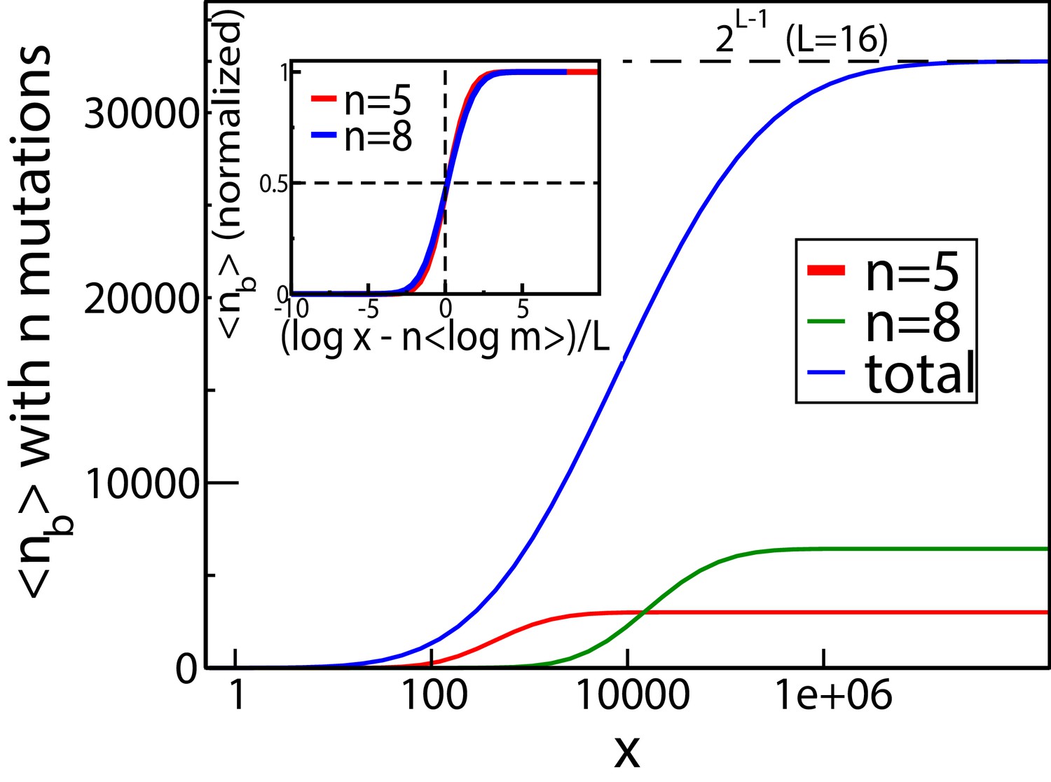
The mean number of genetic backgrounds in which a mutation is beneficial depends on the concentration.
The numerically computed mean number is shown in the blue curve. We also computed the mean for genetic backgrounds with a fixed a number of mutations. The results for two of these values, and are also shown. The inset shows these values of mean as a fraction of the total number of backgrounds with mutations.
Figure 6
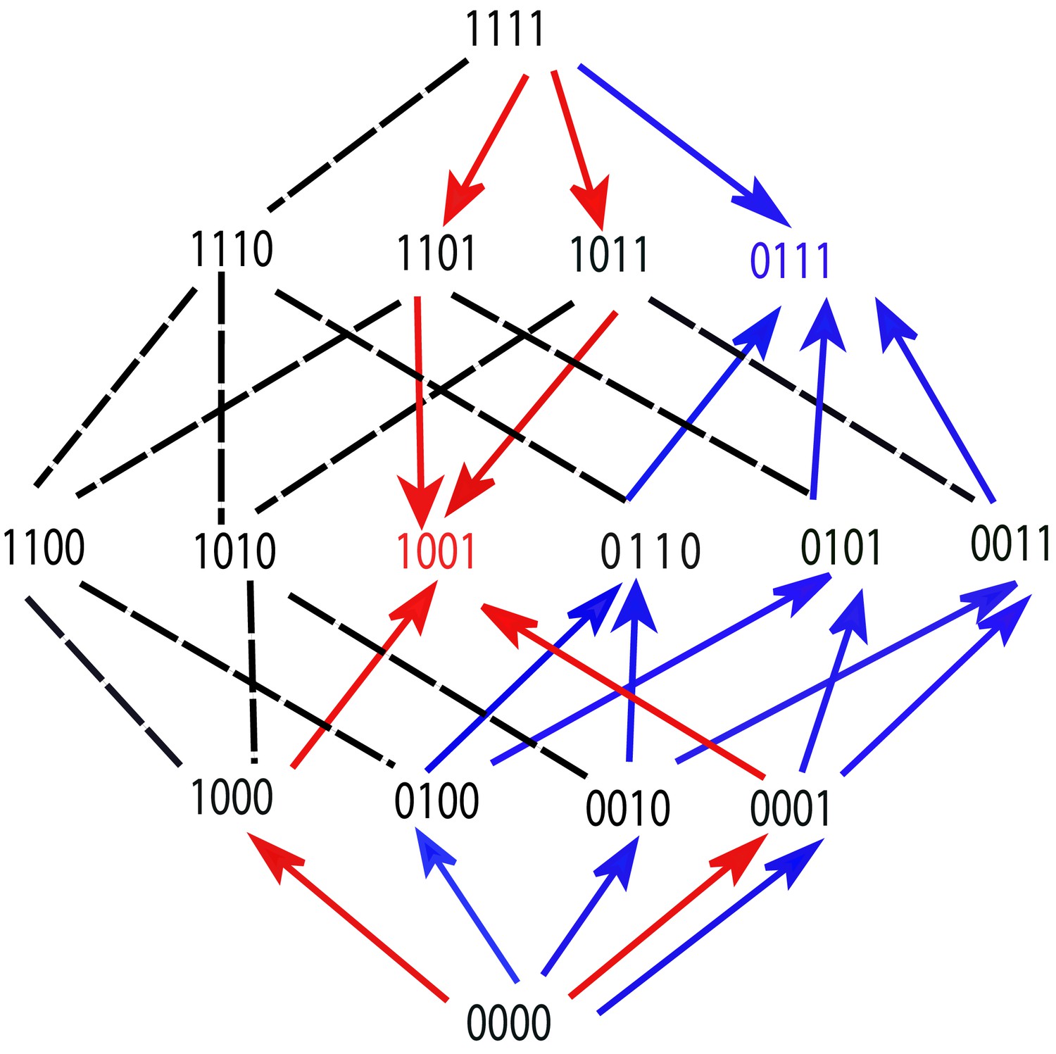
A fitness graph of a landscape with mutations, illustrating the accessibility property.
There are two fitness peaks, 1001 (red) and 0111 (blue). The fitness peaks are accessible from all their subset and superset genotypes following the paths marked by the arrows.
Figure 7
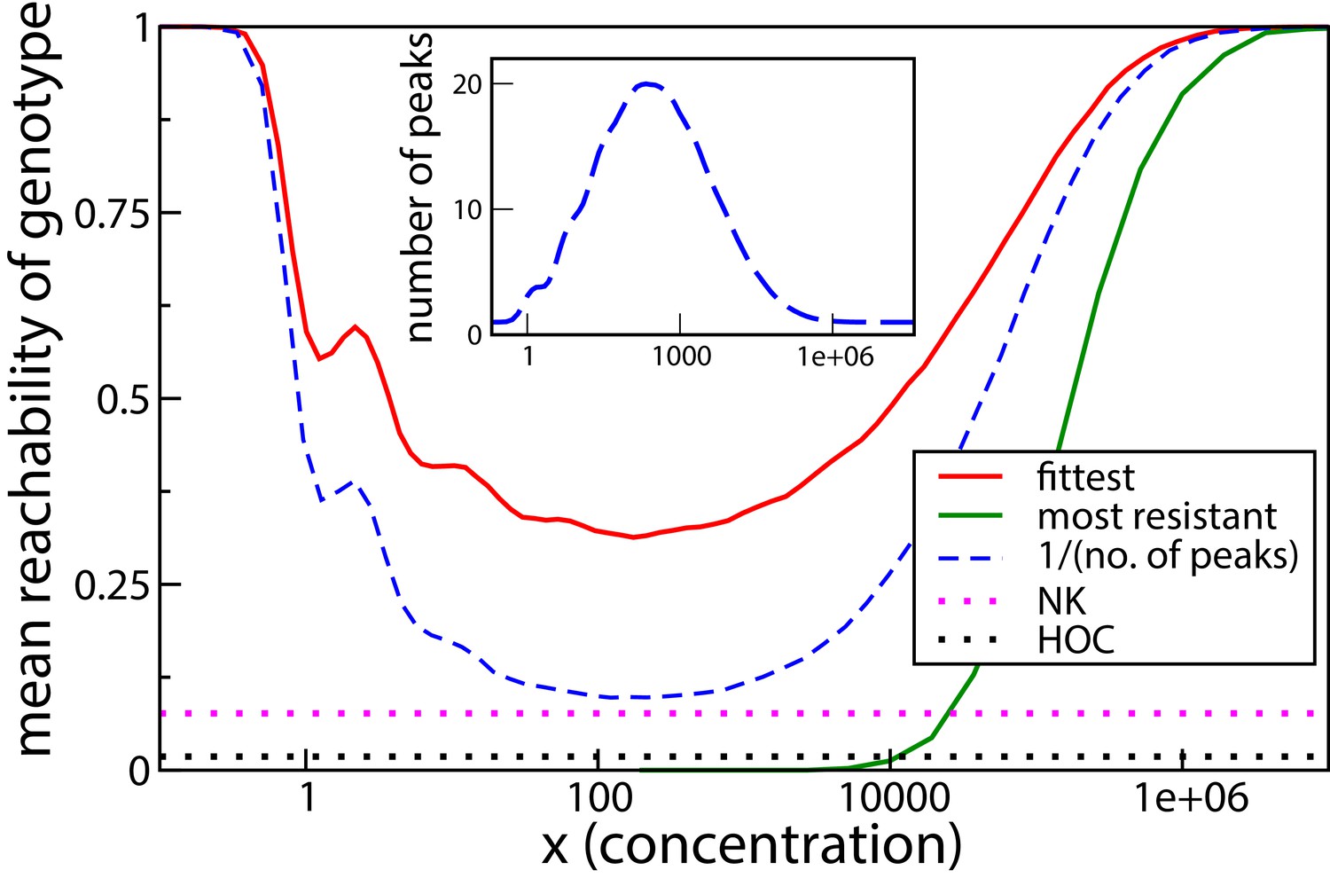
Reachability of fittest genotype and most resistant genotype.
The same model as in the previous subsection has been used, with . Inset shows the mean number of fitness peaks as a function of concentration. Dotted horizontal lines show comparisons to the HoC model and an NK model with the same number of mutations. These models were implemented using an exponential distribution of fitness values.
Figure 8
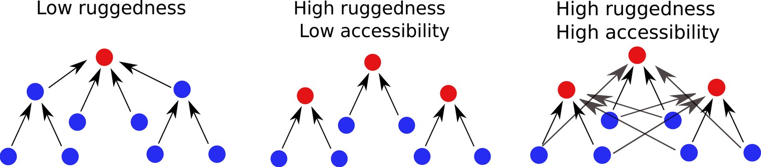
Accessibility and ruggedness in different types of fitness landscapes.
The first two landscapes correspond to the typical cases of smooth and rugged landscapes. The third figure describes landscapes with adaptational tradeoffs, where high ruggedness coexists with high accessibility.
Tables
Table 1
Epistasis in null-fitness and MIC for E. coli in the presence of ciprofloxacin
The table contains a combinatorially complete subset of the data reported by Marcusson et al., 2009, composed of the four mutations S83L (gyrA), D87N (gyrA), marR, and acrR. The names of the strains and values of null-fitness (in competition assays with the wild type) in the third column and MIC (of ciprofloxacin) in the fifth column are obtained from Marcusson et al., 2009. The binary representations follow the same convention as given in the caption of Figure 2. The fourth and sixth columns are respectively the null-fitness and MIC values expected in the absence of epistasis. NA denotes the cases where this is not applicable. The values in parentheses are error estimates. In the third and fifth columns, the errors in the are calculated as , where are the standard error as calculated from the standard deviations reported in the paper. The errors in columns four and six were estimated as where the sum is over the mutations present in the combinatorial mutants. The detectable cases of epistasis are marked in blue. Negative epistasis is found in all these cases. Also, all the cases with epistasis correspond to two or more mutations that affect the same chemical pathways.
| Strain | String | Log null-fitness | Non-epistatic | Log MIC | Non-epistatic |
|---|---|---|---|---|---|
| MG1655 | 00000 | 0.00 (±0.004) | NA | 0.00 (±0.35) | NA |
| LM378 | 10000 | 0.01 (±0.016) | NA | 3.17 (±0.70) | NA |
| LM534 | 01000 | −0.01 (±0.018) | NA | 2.75 (±0.70) | NA |
| LM202 | 00010 | −0.19 (±0.020) | NA | 0.69 (±0.70) | NA |
| LM351 | 00001 | −0.094 (±0.014) | NA | 1.08 (±0.70) | NA |
| LM625 | 11000 | −0.030 (±0.011) | 0.0 (±0.038) | ||
| LM421 | 10010 | −0.15 (±0.019) | −0.18 (±0.040) | 4.13 (±0.70) | 3.56 (±1.1) |
| LM647 | 10001 | −0.051 (±0.013) | −0.084 (±0.034) | 3.44 (±0.70) | 4.65 (±1.1) |
| LM538 | 01010 | −0.19 (±0.020) | −0.20 (±0.042) | 4.13 (±0.70) | 3.46 (±1.1) |
| LM592 | 01001 | −0.083 (±0.015) | −0.10 (±0.036) | 3.16 (±0.70) | 3.83 (±1.1) |
| LM367 | 00011 | −0.20 (±0.026) | −0.28 (±0.038) | 2.06 (±0.70) | 1.77 (±1.1) |
| LM695 | 11010 | −0.24 (±0.017) | −0.19 (±0.058) | ||
| LM691 | 11001 | −0.073 (±0.013) | −0.094 (±0.052) | ||
| LM709 | 10011 | −0.24 (±0.027) | −0.274 (±0.054) | 4.54 (±. 70) | 4.94 (±1.4) |
| LM595 | 01011 | 4.54 (±. 70) | 4.52 (±1.4) | ||
| LM701 | 11011 |
Additional files
Download links
A two-part list of links to download the article, or parts of the article, in various formats.
Downloads (link to download the article as PDF)
Open citations (links to open the citations from this article in various online reference manager services)
Cite this article (links to download the citations from this article in formats compatible with various reference manager tools)
Predictable properties of fitness landscapes induced by adaptational tradeoffs
eLife 9:e55155.
https://doi.org/10.7554/eLife.55155


