Aberrant sorting of hippocampal complex pyramidal cells in type I lissencephaly alters topological innervation
- Program in Developmental Neurobiology, Eunice Kennedy-Shriver National Institute of Child Health and Human Development, National Institutes of Health, United States
- Postdoctoral Research Associate Training Program, National Institute of General Medical Sciences, United States
- Brown University, Department of Neuroscience, United States
Figures
Figure 1

Lis mutants mice display heterotopic banding and ectopic positioning of calbindin-expressing principal cells.
(A) Left, two coronal NeuN stained images from differing levels of dorsal CA1 hippocampus in a wild-type littermate. Right, approximately matched coronal sections from a Lis mutant displaying heterotopic banding of the PCL. Scale bars are 300 μm. (B) Left, wild-type and Lis1-MUT, right, staining of CA1 highlighting the position of the PCL, calbindin-positive neurons, and overlay. Note the deep layer preference of calbindin-expressing neurons, particularly in distal CA1 in mutant. Scale bars are 200 μm. (C) Higher magnification view of the overlay images in (B), for wild-type (left) and Lis1-MUT (right). Scale bars are 150 μm. (D) Normalized histogram showing the positioning of calbindin-expressing cells in mutants with PCL banding compared to wild-type mice. (E) Percentage of cells in deep and superficial layers expressing calbindin in distal CA1 (for controls mice, the single PCL is divided in half radially). Counts represent number of identified calbindin soma divided by number of DAPI identified cells, Wt: deep 8.9 ± 2.8%, superficial 25.1 ± 1.3%; Lis1-MUT: deep 18.0 ± 2.8%, superficial 4.4 ± 1.0%. (F) Same as (E) for proximal CA1, Wt: deep 16.3 ± 2.3%, superficial 30.0 ± 2.0%; Lis1-MUT: deep 12.1 ± 2.3%, superficial 19.0 ± 2.4%; n = 12 Wt and 12 Lis1-MUT slices for distal and 12 and 11 for proximal, from six animals.
-
Figure 1—source data 1
Normalized calbindin cell counts within given regions of interest for distal and proximal CA1, normalized positional counts of CB+ cells.
- https://cdn.elifesciences.org/articles/55173/elife-55173-fig1-data1-v2.xlsx
Figure 2
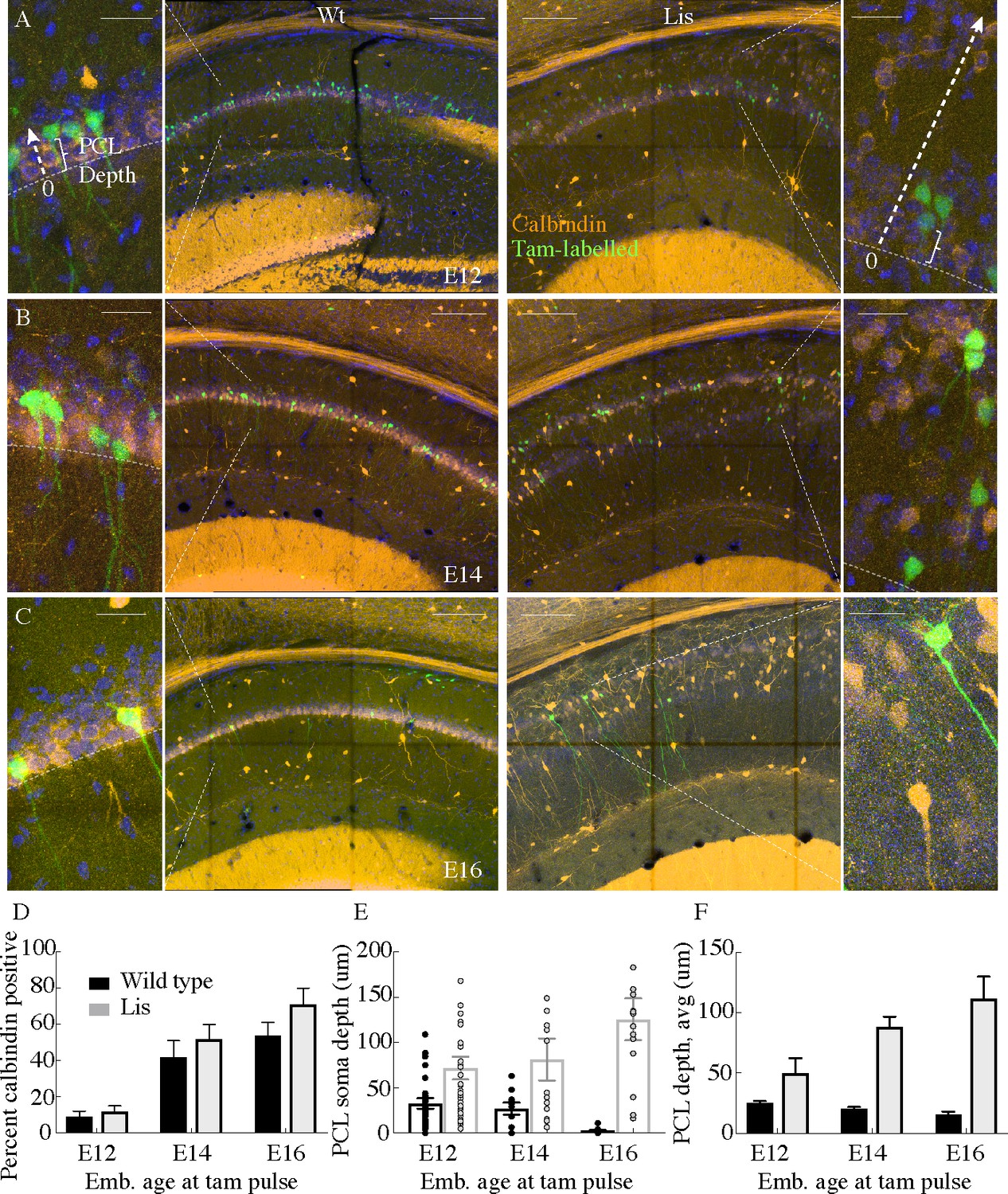
Cellular birth-dating indicates ectopic calbindin cells in Lis mutants are the same late-derived embryologic population.
(A) Wild-type (left) and Lis mutant (right) example birth-dating images for a litter tamoxifen dosed between E12-E13. Note the cutout, displaying how cellular somatic positioning was measured from the front of the PCL (as opposed to normalized structural position). Green corresponds to cells born during tamoxifen administration; orange is calbindin immunohistochemistry staining carried out when litters are P30. (B) Same as in (A) but for litters dosed at E14-E15. (C) Same as (A) but for litters dosed at E16-E17. (D) Quantification of the fraction tamoxifen-marked neurons co-staining for calbindin antibody from each timepoint. E12: Wt: 9 ± 3%; Lis1-MUT: 12 ± 3%, E14: Wt: 42 ± 9%; Lis1-MUT: 52 ± 8%, E16: Wt: 54 ± 7%; Lis1-MUT: 71 ± 9%. (E) Example counts from single images at each timepoint for PCL depth measurements. Later born cells position more superficially (front of the PCL) in non-mutants, but deeper in Lis1-MUT littermates. (F) Group averages for the measurements shown in (E). E12- Wt: 25.4 ± 1.4 μm; Lis1-MUT: 50 ± 12.3 μm, E14- Wt: 20.5 ± 1.3 μm; Lis1-MUT: 88 ± 8.7 μm, E16- Wt: 15.6 ± 2.6 μm; Lis1-MUT -: 111.6 ± 18.3 μm. Scale bars are 150 μm and 25 μm for the main image and zoom, respectively.
-
Figure 2—source data 1
Summary percentage CB+ cells with Tam labelling, PCL depth measurements for cells in single mouse examples, summary data with PCL depths.
- https://cdn.elifesciences.org/articles/55173/elife-55173-fig2-data1-v2.xlsx
Figure 3
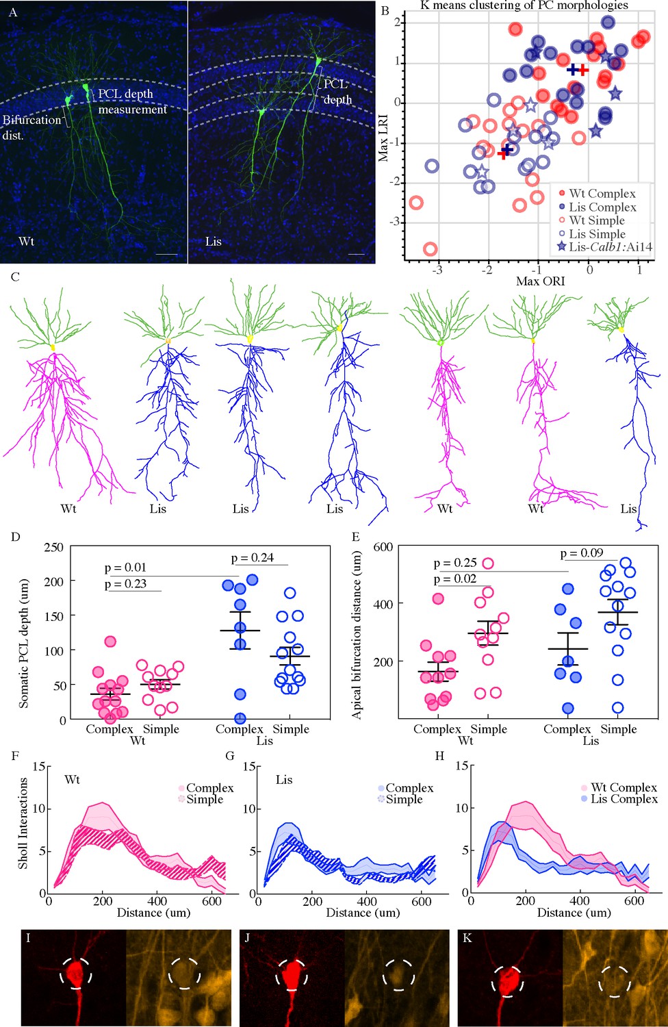
Lis1-MUT calbindin-expressing PCs retain relatively complex morphologies.
(A) Recovered cells from non-mutant and mutant experiments, highlighting different apical dendritic morphologies, complex and simple. Complex morphologies have been previously shown to be highly predictive of calbindin expression (Li et al., 2017). Scale bars are 50 μm. (B) Supervised K-means plots (63 best recovered cells, k = 2) carried out separately for mutant and wild-type data (blue and red respectively). Filled circles correspond to complex morphologies and open circles are simple. Stars are morphological recoveries from Lis1 mutants crossed to a Calb1-cre;Ai14 mouse line (n = 8 total) – filled stars have confirmed calbindin expression and open stars are calbindin negative recordings. These cells are then run through the same clustering algorithm, and the associated LRI/ORI positions are plotted over the original clustering. Note filled and open stars fall in the upper right (complex) quadrant and the lower left (simple) quadrant, respectively. (C) Example morphological reconstructions, ranging from most complex (left) to simple (right). (D) Positional properties for predicted calbindin (complex, filled circles) and non-calbindin expressing (simple, open circles) principal cells. Note predicted calbindin expressing cells were superficial to non-calbindin predicted, and this trend was inverted for Lis1-MUT animals. Wt: complex 36.42 ± 8.5 μm, simple 50 ± 6.9 μm; Lis1-MUT: complex 128 ± 26.6 μm, simple 90.9 ± 12.7 μm, n = 13, 11, 8, 13, respectively. Depth is measured as it was for Figure 2 from the front/superficial side of the PCL. (E) Group sorted measurements for distance along primary apical dendrite until first prominent bifurcation occurs. Wt: complex 163 ± 32.8 μm, simple 295.9 ± 41.4 μm; Lis1-MUT: complex 241.6 ± 55.8 μm, simple 368.9 ± 43.4 μm. Note complex cells tend to bifurcate sooner in both mutant and non-mutants. (F) Sholl interactions from Wt apical dendrites alone, of complex and simple sorted cells. (G) Likewise, for Lis1-MUT animals. (H) Overlay of the complex morphology sholl data from non-mutant and mutant experiments. Despite retaining a relatively complex population, complex Lis1-MUT - principal cells have decreased apical dendritic branching that peaks closer to the soma. (I–K) Somatic images confirming calbindin expression from three recordings performed in Lis1 mutants bred to a Calb1-cre;Ai14 line. Morphologically these cells clustered with the complex group in (B) – filled stars, while calbindin negative recoveries (not shown here) are plotted as open stars in (B). Dashed circle diameter is 15 μm.
-
Figure 3—source data 1
LRI/ORI values from script, and resulting morphological group.
Somatic positions and bifurcation distances.
- https://cdn.elifesciences.org/articles/55173/elife-55173-fig3-data1-v2.xlsx
Figure 4
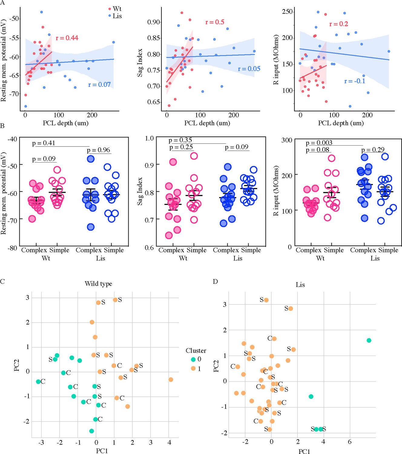
Physiological properties of calbindin positive and negative morphological clusters.
(A) Left, somatic PCL depth correlations with cellular resting membrane potential for wild-type (red) and Lis1-MUT (blue) recordings. Middle, likewise, for sag index, where values closer to 1 correspond to less sag exhibited. Right, same for input resistance. (B) Same data as in (A), grouped by predicted calbindin expression. (C) Supervised K-means (n = 2) sorting wild types. A handful of electrophysiological properties alone are capable of reasonably accurate morphological subtype prediction (and therefore calbindin expression). C’s and S’s correspond to the data points associated morphological group, note that even mis-categorized points are near the midline. Of 8 morphologically complex cells, 6 are found in in physiological cluster 0, of 11 simple cells, 8 are found in physiological cluster 1. (D) Same as in (C) for recordings in Lis mutants. Physiological properties are less capable of predicting morphological cluster in Lis mutant mice.
-
Figure 4—source data 1
Physiological properties by morphological type, position within CA1, and clustering data/results for ephys Kmeans.
- https://cdn.elifesciences.org/articles/55173/elife-55173-fig4-data1-v2.xlsx
Figure 5
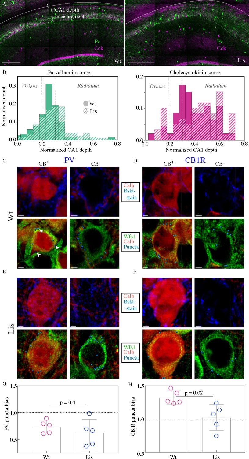
CCK-expressing basket cells have decreased innervation preference with ectopic calbindin-positive principal cells.
(A) Low-magnification images showing the locations of parvalbumin and cholecystokinin-expressing interneurons in the CA1 hippocampus. Note the CA1 depth measurement from the back of the oriens – this measure is more appropriate for assessing somatic position within the larger CA1 structure, as opposed to PCL depth used elsewhere in this study. Scale bars are 350 μm. (B) Normalized histograms of basket cell soma depth measurements along the radial axis of CA1, both PV- (left) and CCK-containing (right) inhibitory interneuron somas show modest superficial shifts in Lis1-MUT mice. (C) High-magnification images of a staining experiment for the quantification of PV-containing inhibitory puncta from control littermate samples. Left, an example CB-expressing principal cell. Right, an example non-CB-expressing principal cell. The top row shows calbindin and parvalbumin staining, the bottom row shows the same cells with calbindin, Wfs1 staining which was used to draw the cell border, and the puncta derived from the parvalbumin staining shown above (arrows point to a few in the first panel) – these puncta are filtered for proximity to a postsynaptic gephyrin puncta (channel not shown). (D) Same as in (C), except the interneuron staining is for the cannabinoid receptor 1, highly expressed in the terminals of CCK-expressing interneurons. (E and F) Same as the corresponding above panels, but for samples from Lis1-MUT littermates. Scale bars are 2 μm. (G) PV puncta bias summary. PV puncta had a modest preference for non-calbindin expressing principal cells in both non-mutant and mutant slices. PV-calbindin preference: 0.74 ± 0.05 and 0.63 ± 0.11 innervation biases for wild-type and mutants, respectively, p=0.55, each point represents 12 cells from a slice, n = 3 pairs of littermates from three litters. (H) Same as in (E), but for experiments where the PV antibody was replaced by the CB1-R antibody. Non-mutant CCK baskets displayed a preference for calbindin-expressing principal cells that was lost in Lis1-MUT mice. CB1-R-calbindin preference: 1.32 ± 0.04, 1.02 ± 0.09 for wild-type and mutant respectively, p=0.02. Scale bars for C-F are 2 μm.
-
Figure 5—source data 1
Summary interneuron positions within CA1.
Inhibitory puncta quanitification for CB+ and CB- somas, in mutant and Wt animals.
- https://cdn.elifesciences.org/articles/55173/elife-55173-fig5-data1-v2.xlsx
Figure 6
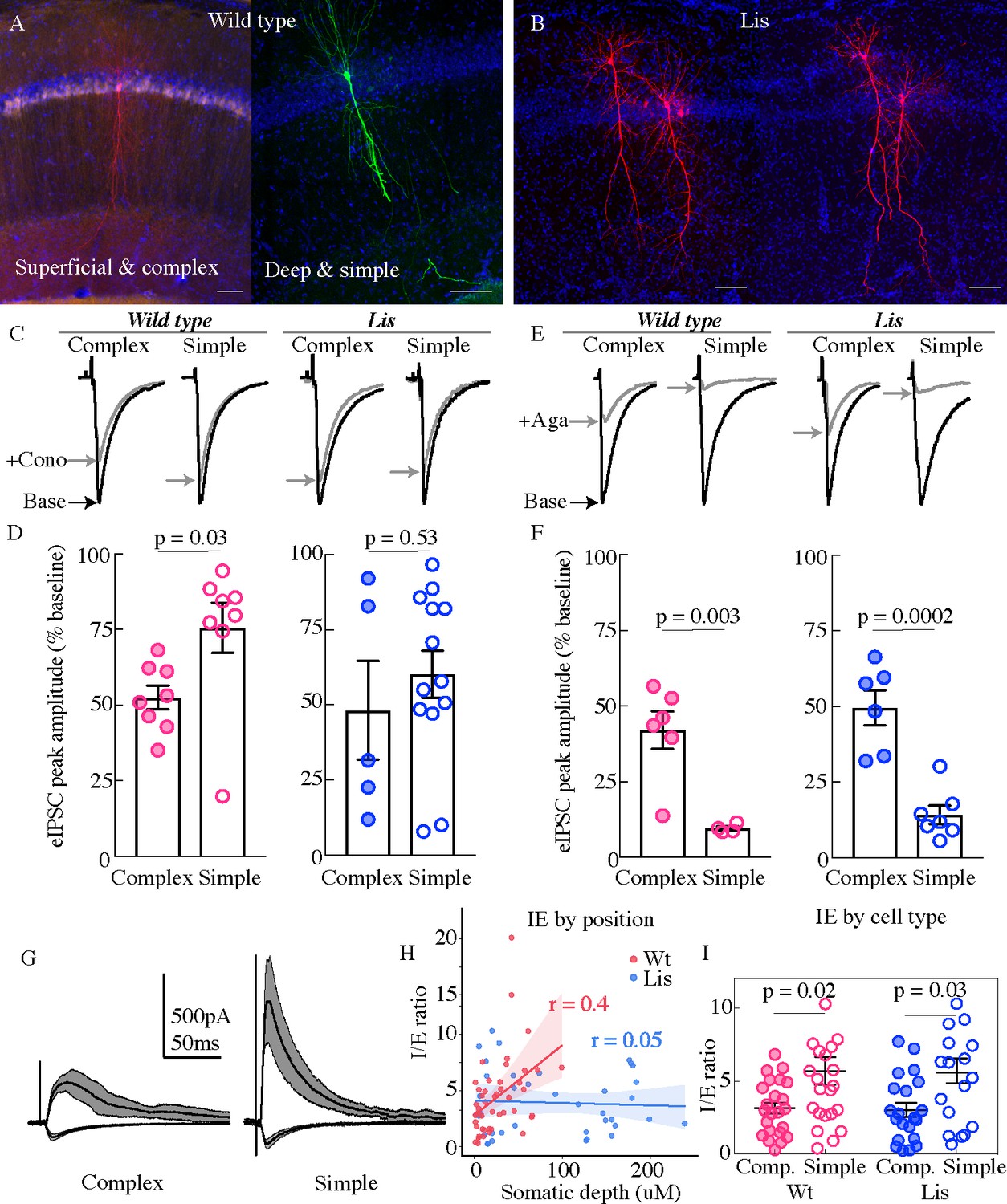
Physiological assays of network function within CA1.
(A and B) Cell recoveries from normal type and Lis1 mutant experiments. Scale bars are 85 μm. (C) Normalized example traces from pre- and post-wash in (dashed) of omega-conotoxin (1 μM), from left to right, a normal-type complex and simple recordings, followed by Lis mutant complex and simple examples. Stimulation for monosynaptic experiments was delivered locally in the CA1 PCL. (D) Quantification of the percent reduction in the evoked IPSC 10–12 mins after drug application. Wt: complex 52.5 ± 3.9%, simple 75.6 ± 8.3%; Lis1-MUT: complex 48.2 ± 16.4%; simple 60.2 ± 7.8%, n = 8, 8, 13, 5, respectively. (E) Example traces as in (C) but for omega-agatoxin experiments (250 nM). (F) As in (D) but for agatoxin. Wt: complex 42.0 ± 6.2%, simple 9.5 ± 0.7%; Lis1-MUT: complex 49.6 ± 5.8%; simple 14.2 ± 3.0%, n = 6, 4, 6, 7, respectively. (G) Example traces for monosynaptic EPSCs (excitatory, inward current), and disynaptic feedforward IPSCs (inhibitory, outward current) evoked by stimulation of Schaffer collaterals, from a simple and complex recovered cell morphology in normal type. (H) IPSC amplitude/EPSC amplitude plotted by somatic PCL depth. (I) Same data as in (H) sorted by cell sub-type. Wt: complex 3.15 ± 0.39, simple 5.70 ± 0.95; Lis1-MUT: complex 3.02 ± 0.49%; simple 5.03 ± 0.76, n = 23, 23, 21, 17, respectively.
-
Figure 6—source data 1
Monosynaptic wash-in event reduction percentages; disynaptic data summary and IE ratios with assigned morphological group.
- https://cdn.elifesciences.org/articles/55173/elife-55173-fig6-data1-v2.xlsx
Figure 7
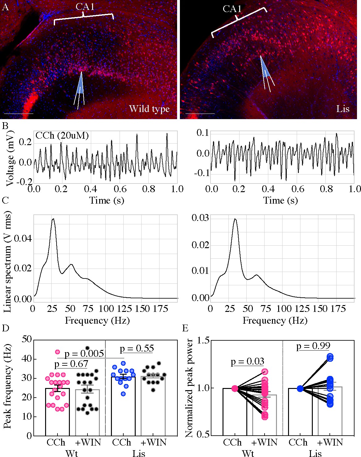
Lis mutants display robust carbachol-induced oscillations.
(A) Normal type (left) and mutant (right) images from ventral hippocampus in Calb1-cre:Ai14 mice. Note the second layer of deeply positioned calbindin expressing principal cells in the Lis mutant. Scale bars are 200 μm. (B) One second of data during carbachol induced activity from radiatum side electrodes in normal type and mutant recordings, respectively. (C) Power spectra computed for each of the above example recordings. (D) Summary peak frequency data for wild-type and Lis mutant experiments, in carbochol alone, and with addition of WIN-55 (Cb1-R agonist, 2 um). Wt CCh 24.88 ± 1.7 Hz, +WIN 24.4 ± 2 Hz, Lis1-MUT CCh 31 ± 1.1 Hz, +WIN 31.3 ± 1 Hz. (E) Summary data as in (D) but for normalized Vrms power at the peak frequency. Wt +WIN 0.93 ± 0.03 vs CCh alone p=0.03, Lis1-MUT +WIN 1.02 ± 0.04 vs CCh alone p 0.69; n = 20 and 14 wild-type and mutant respectively. Pre-vs-post wash p values represent paired t tests.
-
Figure 7—source data 1
Peak frequency and peak power summary data., note we normalize power data with-in exp.
- https://cdn.elifesciences.org/articles/55173/elife-55173-fig7-data1-v2.xlsx
Figure 8

Carbachol oscillations in Lis1 mutants are less synchronous across CA1 heterotopias.
(A) Normal type (left) and mutant (right) images from ventral hippocampus showing the positioning of dual electrode recordings, one from the s. radiatum and a second s. oriens side electrode in the same radial plane. Scale bars are 200 μm. (B) One second of simultaneous recordings from the deep (top) and superficial (bottom) electrodes, for wild-type (left) and Lis mutant (right) example experiments. Dashed lines highlight peak alignment between electrodes – note the blue line intersecting near a trough in the top trace, and a peak in the bottom. (C) Cross correlation plots for the example experiments shown in (B). Correlation values are arbitrary units. (D) Summary data for non-mutant and Lis1-MUT experiments in carbachol and after WIN-55 wash-in. Wt CCh 394.6 ± 80, +WIN 333.9 ± 72, Lis1-MUT CCh 394.2 ± 60.8, +WIN 427.2 ± 84.1. (E) Summary for the millisecond timing of peak correlation shifts shown in (D). Wt CCh 1 ± 0.8 ms, +WIN 0.68 ± 0.5 ms, Lis1-MUT CCh −1.8 ± 0.8 ms, +WIN −0.4 ± 1.23 ms; n = 20 and 14 wild-type and mutant respectively. Pre-vs-post wash p values represent paired t tests.
-
Figure 8—source data 1
Cross correlation and temporal shift data.
- https://cdn.elifesciences.org/articles/55173/elife-55173-fig8-data1-v2.xlsx
Author response image 1
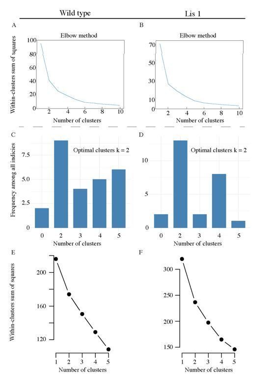
Pre-clustering analysis for morphological and physiological supervised clustering.
(A) An elbow plot of the total within-cluster sum of squares over various supervised clustering values of k, for morphological LRI and ORI values in Figure 3B. (B) Likewise for Lis1 mutant data. (C) and (D) display summary histograms generated from nbclust, the plots suggest that the optimal cluster answer is k = 2 for both mutant and non-mutant data. (E) An elbow plot of the total within-cluster sum of squares over various supervised clustering values of k, for the physiological properties analyzed in Figure 4C. (F) Likewise, for Lis1 mutant data in Figure 4D.
Additional files
-
Source code 1
Code used to cluster and sort cellular morphologies.
- https://cdn.elifesciences.org/articles/55173/elife-55173-code1-v2.ipynb
-
Transparent reporting form
- https://cdn.elifesciences.org/articles/55173/elife-55173-transrepform-v2.docx
Download links
A two-part list of links to download the article, or parts of the article, in various formats.
Downloads (link to download the article as PDF)
Open citations (links to open the citations from this article in various online reference manager services)
Cite this article (links to download the citations from this article in formats compatible with various reference manager tools)
Aberrant sorting of hippocampal complex pyramidal cells in type I lissencephaly alters topological innervation
eLife 9:e55173.
https://doi.org/10.7554/eLife.55173


