Spatiotemporal dynamics of multi-vesicular release is determined by heterogeneity of release sites within central synapses
Figures
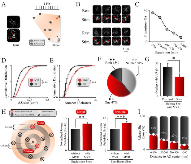
Non-uniform spatial features of MVR events and release sites within an AZ.
(A) Sample spatial distribution of ten UVR events and a single MVR (arrows) event within a hippocampal bouton evoked by 120 APs at 1 Hz. Release sites were defined using a hierarchical clustering algorithm with a cluster diameter of 50 nm (Maschi and Klyachko, 2017) and are shown by crossed circles. Images (before and after 1 AP stimulation) show a sample MVR event highlighted by arrows. (B) Examples of MVR events in different boutons. (C) Proportion of MVR events as a function of intra-event separation distances. (D, E) Cumulative distributions of AZ area (D) and number of clusters/release sites (E) for all recorded boutons (black) and boutons exhibiting MVR events (red). (F) Spatial overlap of MVR and UVR events. Percentages of MVR events in which none, one or both events in the pair occurred at release sites that also harbored at least one UVR event. (G) Probability of reuse by UVR events of more proximal vs. more distal release sites engaged in MVR event pairs. (H) Analysis of release probability (Pr-site) of more distal (left bars) and more proximal (right bars) release sites engaged in MVR event pairs compared to other release sites equidistant to the AZ center within ±25 nm but not engaged in the MVR event during the observation period (shown schematically on the left). (I) Proportion of release sites that are reused at least once during the observation period as a function of the distance to the AZ center. Numbers shown represent average release site re-use in a given bin. N = 3781 (UVR) and 245 (MVR) events, from 90 dishes from 11 independent cultures; *p<0.05, **p<0.01, ***p<0.001. Two-sample KS-test (D, E); Chi-square test (G); Paired t-test (H).
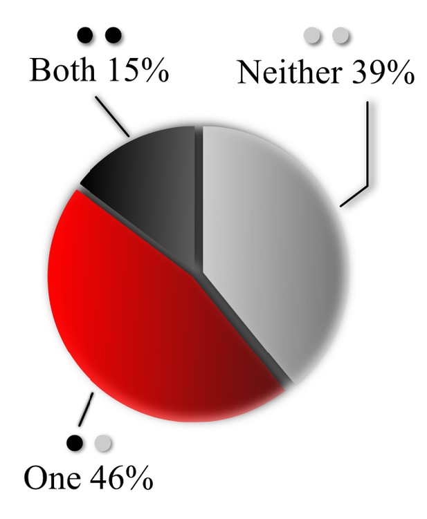
Overlap of MVR and UVR events determined by proximity analysis.
Percentage of MVR events in which none, one or both events in the pair overlapped (within 25 nm) with at least one UVR event during observation period, as determined by proximity analysis.
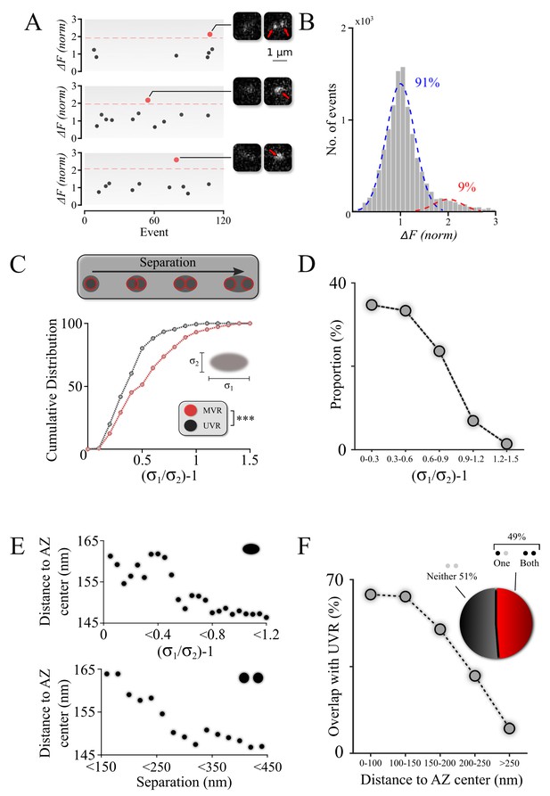
Spatiotemporal features of resolved MVR events generalize to unresolved MVR events.
(A) MVR (red) and UVR (black) events were separated on the basis of the event amplitude. Examples of an identified resolved MVR event (top) and two unresolved MVR events (middle and bottom) are shown with corresponding images. (B) An intensity histogram for all detected events from panel (A) reflects the quantal nature of fusion events. Gaussian fits to the first peak (UVR events, blue) and second peak (MVR events, red) and their relative abundances are shown. (C) Asymmetry analysis of unresolved MVR events vs UVR events. The asymmetry score was calculated using asymmetrical Gaussian fit to the event image to determine maximal (δ1) and minimal (δ2) width (insert). (D) Proportion of unresolved MVR events as a function of asymmetry score, which correlates with intra-event separation distances. (E) Mean distance to the AZ center for unresolved (top) and resolved (bottom) MVR events. Distance was calculated from the peak of the Gaussian fit for unresolved MVR events and from the center of the line connecting two fusions within the resolved MVR events. (F) Probability of overlap of unresolved MVR and UVR events in the same bouton as a function of distance to the AZ center. Event overlap was determined using proximity analysis with a radius of 25 nm. Only more symmetrical MVR events (asymmetry score <0.5) were included in this analysis. Points represent the proportion of MVR events within a given distance band that overlapped with UVR events. Pie chart: proportion of unresolved MVR events that overlap or not with UVR events during the observation period. N = 151 (UVR) and 144 (MVR) events, 90 dishes from 11 independent cultures. *** p<0.001; Two-sample KS-test (C).
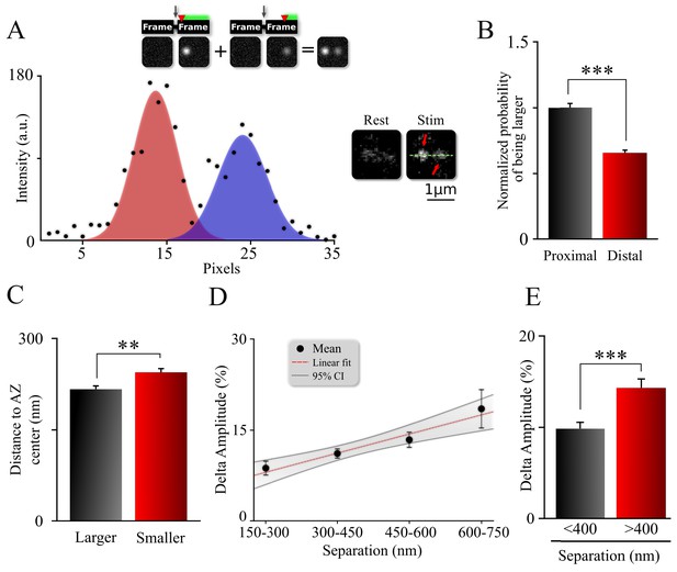
Spatiotemporal organization of release events comprising an MVR.
(A) Sample image (right) and intensity profile (left) of an MVR event with noticeable difference in intra-event amplitude. The top insert shows a cartoon representation of a relationship between a time delay (red arrow) of the second fusion after an action potential and the resulting amplitude difference within an MVR event. (B) Probability that the proximal or distal event within MVR pairs is larger, normalized to that of the proximal event. (C) Distance to the AZ center from the larger and smaller events within MVR pairs. (D, E) Amplitude difference of the two events comprising MVR as a function of intra-event separation. Linear fit (D) and t-test of pooled data (E) are shown. *p<0.05, ***p<0.001; Chi-square test (B); Paired t-test (C); Two-sample t-test (E). N = 245 MVR events, from 90 dishes from 11 independent cultures.

Amplitude difference within the MVR event pairs is not due to measurement uncertainty, changes in vesicle size or cleft pH within the AZs.
(A) Uncertainty in the fusion event amplitude determination was estimated on the basis of the amplitude variation of consecutive UVR events evoked in the same bouton at 1 Hz. Uncertainty in determination of individual event amplitude does not account for the amplitude differences observed in MVR events with large separation. (B) Amplitude of UVR events as a function of the distance to the AZ center. No correlation was found between event amplitude and distance to AZ center (p=0.21, linear fit). The bar graph shows that no significant difference in amplitude exists between central events (pooled data for 0–100 nm) vs. peripheral events (pooled data for 200–300 nm). (C, D) Vesicle diameter as a function of distance to the AZ center was determined for all vesicles positioned within 100 nm from the AZ (defined previously as tethered vesicles; Maschi et al., 2018) from LaSEM micrographs of hippocampal cultures (EM data from Maschi et al., 2018). Distance from the vesicle to the AZ center was determined from the projection of the vesicle center position onto the AZ plane (C). Vesicle diameter did not show significant changes with distance from the AZ center (p=0.16, linear fit). ***p<0.001; ns, not significant. Two-sample t-test (A,B).
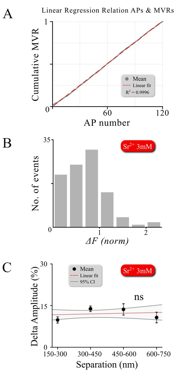
Double events do not result from asynchronous release overlapping temporally with synchronous events.
(A) MVR events occur at the same rate throughout the 120 action potential stimulus at 1 Hz, showing absolutely no increase in double event probability during the train, as would be expected if these events are generated by asynchronous release. (B) An amplitude histogram for asynchronous release events detected in 3 mM Sr+2 after single APs using 1 Hz 120 AP stimulation shows the loss of quantal homogeneity of asynchronous fusion events (with a left-shifted non-Gaussian distribution). This is distinct from the Gaussian amplitude distribution that we observed for synchronous MVR or UVR events in our measurements. (C) Amplitude difference of two asynchronous events detected in the same frame in the same bouton in the presence of 3 mM Sr2+ as a function of intra-event separation. In contrast to MVR events, no correlation was found between spatial event separation and desynchronization (p=0.662).
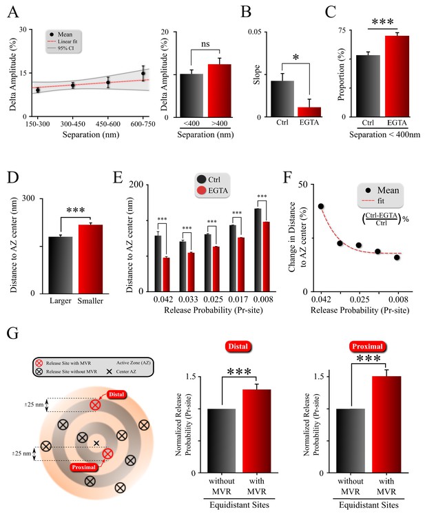
Spatiotemporal features of MVR events and release site properties are calcium-dependent.
(A) Effect of EGTA on the correlation between the spatial separation and amplitude difference between two events comprising an MVR. (B) The effect of EGTA was assessed by comparing the slopes of the correlation in panel (A) in control (from Figure 3D) and EGTA (from A) conditions. (C) Proportion of MVR events with intra-event separation <400 nm in EGTA and control conditions. (D) Distance to the AZ center from the larger and smaller events within MVR pairs in the presence of EGTA. (E,F) Average distance to the AZ center (E) and its relative change (F) for individual release sites binned on the basis of their release probability, in EGTA and control conditions. (G) Release probability of more distal (left bars) and more central (right bars) release sites engaged in MVR event pairs compared to all other release sites equidistant to the AZ center within ±25 nm, in the presence of EGTA. ***p<0.001; ns, not significant. Statistical tests were as follows: two-sample t-test (A,E); one-way analysis of covariance (ANOCOVA) (B); Chi-square test (C); and Paired t-test (D,G). Control: N = 245 MVR events from 90 dishes from 11 independent cultures. EGTA: N = 225 MVR events from 57 dishes from 11 independent cultures.
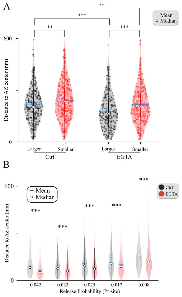
Violin plots of the amplitude differences within MVR event pairs and the effects of EGTA.
(A) Distance to the AZ center from the larger and smaller events within MVR pairs in control (data from Figure 3C) and EGTA conditions (data from Figure 4D). (B) Average distance to the AZ center of individual release sites binned on the basis of their release probability, in control and EGTA conditions (data from Figure 4E). ∗∗p<0.01; ∗∗∗p<0.001. Two-sample t-test.
Tables
Data values and statistical analyses.
Columns represent (from left to right): figure/panel number; experimental conditions; number of samples (synapses, dishes and cultures); mean values and standard errors of the means (SEM); statistical test used for comparison; and the P-value resulting from the statistical comparison.
| Figure number | Conditions | NSyn | NDishes | NCultures | Mean ± SEM | Statistical test | Pval |
|---|---|---|---|---|---|---|---|
| Figure 1D | All | 3781 | 90 | 11 | 0.1014 ± 0.0009 | Two-sample KS-test | <0.001 |
| MVR | 245 | 90 | 11 | 0.164 ± 0.005 | |||
| Figure 1E | All | 3781 | 90 | 11 | 6.57 ± 0.05 | Two-sample KS-test | <0.001 |
| MVR | 245 | 90 | 11 | 9.8 ± 0.03 | |||
| Figure 1G | Proximal | 245 | 90 | 11 | 0.45 ± 0.05 | Chi-square test | 0.0386 |
| Distal | 245 | 90 | 11 | 0.29 ± 0.05 | |||
| Figure 1H | Distal MVR/UVR | 66 | 90 | 11 | 1.24 ± 0.09 | Paired t-test | 0.006 |
| Proximal MVR/UVR | 95 | 90 | 11 | 1.28 ± 0.08 | Paired t-test | <0.001 | |
| Figure 2C | UVR | 151 | 90 | 11 | 0.32 ± 0.02 | Two-sample KS-test | <0.001 |
| MVR | 144 | 90 | 11 | 0.47 ± 0.02 | |||
| Figure 3B | Proximal MVR/Proximal MVR | 245 | 90 | 11 | 1 ± 0.03 | Chi-square test | 0.017 |
| Distal MVR/Proximal MVR | 245 | 90 | 11 | 0.65 ± 0.02 | |||
| Figure 3C | Larger MVR | 245 | 90 | 11 | 214 ± 7 | Two-sample t-test | 0.0058 |
| Smaller MVR | 245 | 90 | 11 | 242 ± 7 | |||
| Figure 3D | MVR | 245 | 90 | 11 | y = 3.108+0.02106 x | Linear fit | <0.001 |
| Figure 3E | MVR <400 nm | 129 | 90 | 11 | 9.8 ± 0.7 | Two-sample t-test | <0.001 |
| MVR >400 nm | 115 | 90 | 11 | 14.3 ± 0.9 | |||
| Figure 4A | EGTA MVR Linear fit | 225 | 57 | 11 | y = 8.801+0.00556 × | Linear fit | 0.264 |
| MVR <400 nm | 156 | 57 | 11 | 10.1 ± 0.8 | Two-sample t-test | 0.131 | |
| MVR >400 nm | 69 | 57 | 11 | 12.3 ± 1.2 | |||
| Figure 4B | Ctrl MVR | 245 | 90 | 11 | 0.021 ± 0.005 | One-way analysis of covariance (ANOCOVA) | 0.022 |
| EGTA MVR | 225 | 57 | 11 | 0.006 ± 0.005 | |||
| Figure 4C | Ctrl MVR | 245 | 90 | 11 | 52 ± 3 | Chi-square test | <0.001 |
| EGTA MVR | 225 | 57 | 11 | 69 ± 3 | |||
| Figure 4D | Larger MVR | 225 | 57 | 11 | 178 ± 7 | Two-sample t-test | <0.001 |
| Smaller MVR | 225 | 57 | 11 | 216 ± 7 | |||
| Figure 4E | Ctrl Pr = 0.042 | 2417 | 90 | 11 | 104 ± 8 | Two-sample t-test | <0.001 |
| EGTA Pr = 0.042 | 2338 | 57 | 11 | 62 ± 5 | |||
| Ctrl Pr = 0.033 | 2417 | 90 | 11 | 93 ± 3 | Two-sample t-test | <0.001 | |
| EGTA Pr = 0.033 | 2338 | 57 | 11 | 72 ± 2 | |||
| Ctrl Pr = 0.025 | 2417 | 90 | 11 | 107 ± 2 | Two-sample t-test | <0.001 | |
| EGTA Pr = 0.025 | 2338 | 57 | 11 | 83 ± 1 | |||
| Ctrl Pr = 0.017 | 2417 | 90 | 11 | 124 ± 1 | Two-sample t-test | <0.001 | |
| EGTA Pr = 0.017 | 2338 | 57 | 11 | 100 ± 1 | |||
| Ctrl Pr = 0.008 | 2417 | 90 | 11 | 154.6 ± 0.7 | Two-sample t-test | <0.001 | |
| EGTA Pr = 0.008 | 2338 | 57 | 11 | 129.8 ± 0.8 | |||
| Figure 4F | Ctrl MVR | 2417 | 90 | 11 | Fit | 0.0030 | |
| EGTA MVR | 2338 | 57 | 11 | a = 17.951 | |||
| b = 1.0049e+09 | |||||||
| c = 5.5575 | |||||||
| Figure 4G | Distal MVR/UVR | 52 | 57 | 11 | 1.29 ± 0.09 | Paired t-test | 0.0020 |
| Proximal MVR/UVR | 77 | 57 | 11 | 1.5 ± 0.1 | Paired t-test | <0.001 | |
| Figure 3—figure supplement 1A | UVR | 136 | 90 | 11 | 11.5 ± 0.8 | Two-sample t-test | 0.1262 |
| MVR,<400 nm | 129 | 90 | 11 | 9.8 ± 0.7 | |||
| UVR | 136 | 90 | 11 | 11.5 ± 0.8 | Two-sample t-test | 0.0232 | |
| MVR,>400 nm | 115 | 90 | 11 | 14.3 ± 0.9 | |||
| Figure 3—figure supplement 1B | UVR | 665 | 90 | 11 | y = 35.088-0.0064674 x | Linear fit | 0.207 |
| UVR 0–100 nm | 285 | 90 | 11 | 34.9±0.6 | Two-sample t-test | 0.1376 | |
| UVR 200–300 nm | 109 | 90 | 11 | 33.4 ± 0.9 | |||
| Figure 3—figure supplement 1D | Synaptic vesicle diameters | NSyn = 93 NVesic = 806 | – | 3 | y = 48.109+0.0047331x | Linear fit | 0.161 |
| Figure 4—figure supplement 1A | Larger Ctrl MVR | 245 | 90 | 11 | 214 ± 7 | Two-sample t-test | 0.0058 |
| Smaller Ctrl MVR | 245 | 90 | 11 | 242 ± 7 | |||
| Larger EGTA MVR | 225 | 57 | 11 | 178 ± 7 | Two-sample t-test | <0.001 | |
| Smaller EGTA MVR | 225 | 57 | 11 | 216 ± 7 | |||
| Larger Ctrl MVR | 245 | 90 | 11 | 214 ± 7 | Two-sample t-test | <0.001 | |
| Larger EGTA MVR | 225 | 57 | 11 | 178 ± 7 | |||
| Smaller Ctrl MVR | 245 | 90 | 11 | 242 ± 7 | Two-sample t-test | 0.0116 | |
| Smaller EGTA MVR | 225 | 57 | 11 | 216 ± 7 | |||
| Figure 4—figure supplement 1B | Ctrl Pr = 0.042 | 2417 | 90 | 11 | 104 ± 8 | Two-sample t-test | <0.001 |
| EGTA Pr = 0.042 | 2338 | 57 | 11 | 62 ± 5 | |||
| Ctrl Pr = 0.033 | 2417 | 90 | 11 | 93 ± 3 | Two-sample t-test | <0.001 | |
| EGTA Pr = 0.033 | 2338 | 57 | 11 | 72 ± 2 | |||
| Ctrl Pr = 0.025 | 2417 | 90 | 11 | 107 ± 2 | Two-sample t-test | <0.001 | |
| EGTA Pr = 0.025 | 2338 | 57 | 11 | 83 ± 1 | |||
| Ctrl Pr = 0.017 | 2417 | 90 | 11 | 124 ± 1 | Two-sample t-test | <0.001 | |
| EGTA Pr = 0.017 | 2338 | 57 | 11 | 100 ± 1 | |||
| Ctrl Pr = 0.008 | 2417 | 90 | 11 | 154.6 ± 0.7 | Two-sample t-test | <0.001 | |
| EGTA Pr = 0.008 | 2338 | 57 | 11 | 129.8 ± 0.8 |


