Low-frequency neural activity reflects rule-based chunking during speech listening
- Key Laboratory for Biomedical Engineering of Ministry of Education, College of Biomedical Engineering and Instrument Sciences, Zhejiang University, China
- Research Center for Advanced Artificial Intelligence Theory, Zhejiang Lab, China
Figures
Figure 1
Stimuli and task.
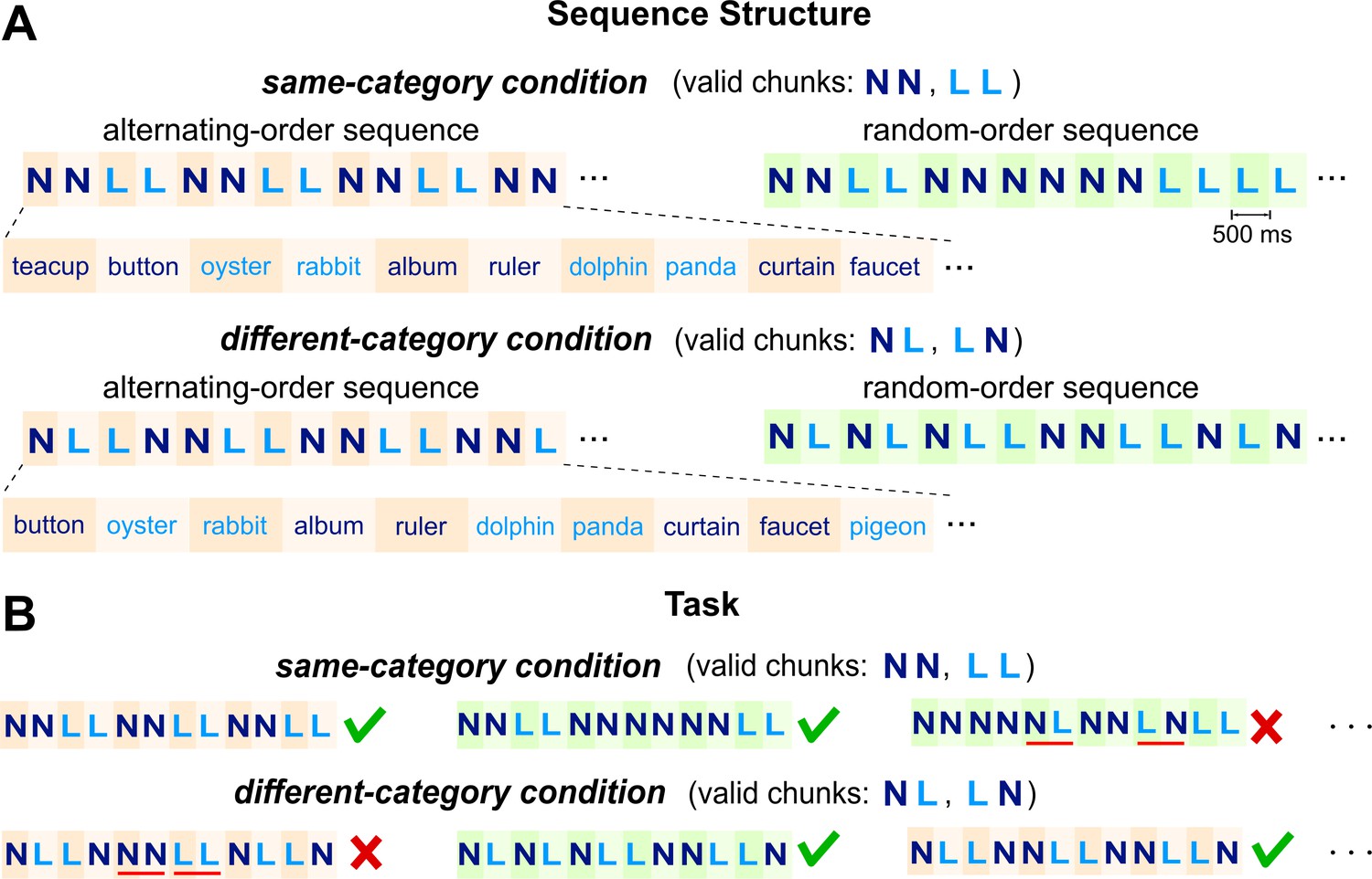
(A) Stimuli consist of isochronously presented nouns, which belong to two semantic categories, that is living (L) or nonliving (N) things. Two nouns construct a chunk and the chunks further construct sequences. In the same-category condition (upper panel), nouns in a chunk always belong to the same semantic category. In the different-category condition (lower panel), nouns in a chunk always belong to different categories. Sequences in each condition further divide into alternating-order (left) and random-order (right) sequences. The alternating-order sequence only differs by a time lag between the same- and different-category conditions. In the illustration, colors are used to distinguish words from different categories and the two words in a chunk but in the speech stimulus all words are synthesized in the same manner. (B) The task is to decompose each sequence into two-word chunks and detect invalid chunks. Three trials and the correct responses are shown for each condition (tick and cross for normal and outlier trials, respectively). Red underlines highlight the invalid chunks.
Figure 2 with 1 supplement
Model simulations.
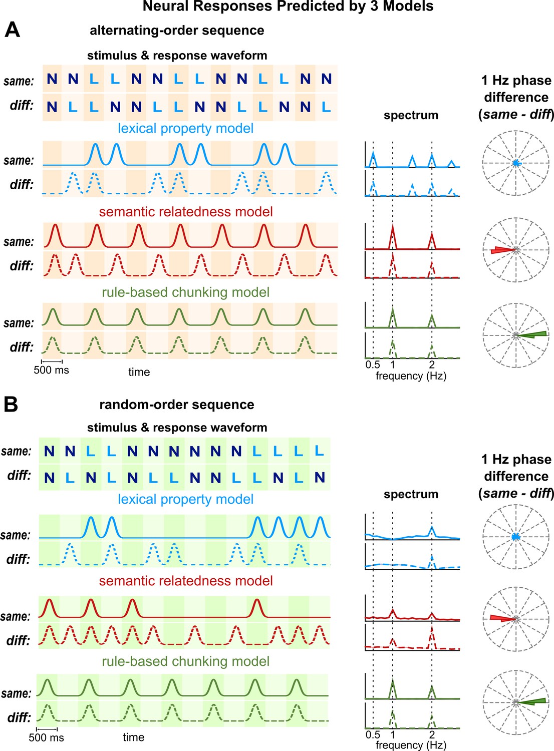
(A) Simulations for alternating-order sequences. The left panel illustrates the response waveform for example sequences. Neural responses predicted by the lexical property and semantic relatedness models differ by a time lag between same- and different-category conditions. The rule-based chunking model, however, predicts identical responses in both conditions. The middle panel shows the predicted spectrum averaged over all sequences in the experiment. The semantic relatedness model and the rule-based chunking model both predict a significant 1 Hz response, while the lexical property model predicts a significant response at 0.5 Hz and its odd order harmonics. The right panel shows predicted phase difference between same- and different-category conditions at 1 Hz. The phase difference predicted by the lexical property model is uniformly distributed. The semantic relatedness model predicts a 180° phase difference between conditions, while the rule-based chunking model predicts a 0° phase difference. (B) Simulations for random-order sequences. The semantic relatedness model and rule-based model predict a significant 1 Hz response. They generate different predictions, however, about the 1 Hz phase difference between conditions.
Figure 2—figure supplement 1

Model simulation.
(A) Procedures to simulate the lexical property model and the semantic relatedness model. The left panel illustrates the representation of word features. Each feature dimension is represented by a pulse sequence, with a pulse placed at the onset of each word and the amplitude of the pulse modulated by the word feature. Two feature dimensions are illustrated here. The predicted neural response is simply the feature sequence convolving a response function, which is a 500 ms Gaussian window. For the semantic relatedness model, the correlation coefficient between binary vectorial word representations is used to measure semantic similarity between words. In the pule sequence, the pulse at the onset of each word denoted the one minus the correlation between the current word and the previous word. (B) Potential waveforms for the chunk response. The rule-based chunking model only assumes a reliable response to each chunk and does not constrain the response waveform. Simulations show that the core model predictions, that is a 1 Hz spectral peak and a 180° phase difference between conditions, are not affected by the response waveform.
Figure 3 with 1 supplement
MEG responses.
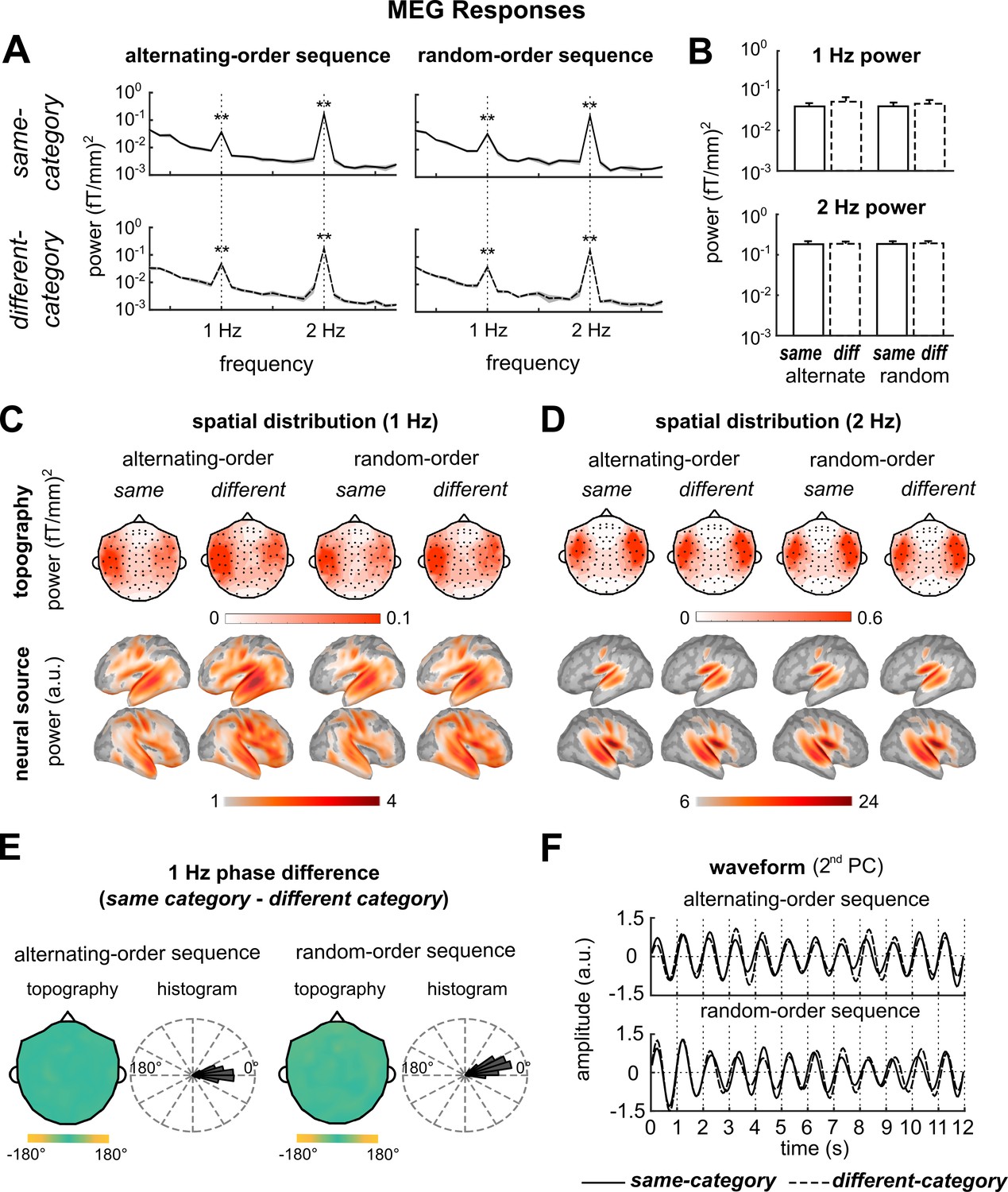
(A) The response power spectrum averaged over participants and MEG gradiometers. A 1 Hz response peak and a 2 Hz response peak are observed. The shaded area covered 1 SEM over participants on each side. (B) The 1 Hz and 2 Hz response power. There is no significant difference between conditions. (C, D) Response topography (gradiometers) and source localization results, averaged over participants. Sensors (shown by black dots) and vertices that have no significant response (p>0.05; F-test; FDR corrected) are not shown in the topography and localization results. The 1 Hz and 2 Hz responses both show bilateral activation. The neural source localization results are shown by the dSPM values and vertices with dSPM smaller than the min value in the color bar are not shown. (E) Phase difference between the same-category and different-category conditions at 1 Hz. The topography shows the distribution of phase difference across MEG sensors (one magnetometers and two gradiometers in the same position are circular averaged). The topography is circular averaged over participants. The histogram shows the phase difference distribution for all 306 MEG sensors. The phase difference is closer to 0° (predicted by the rule-based chunking model) than 180° (predicted by the semantic relatedness model). (F) Waveform averaged over trials and subjects (the second PC across MEG sensors). The waveform is filtered around 1 Hz and is highly consistent between the same- and the different-category conditions. *p<0.05, **p<0.005
Figure 3—figure supplement 1

Additional MEG results.
(A) Individual response spectrum and phase difference. In the response spectrum, each curve is the result from a participant (averaged over alternating- and random-order sequences with both same- and different-category chunks). A 1 Hz spectral peak can be seen in 14 out of 16 participants. In the phase difference (averaged over alternating- and random-order sequences), each point on the unit circle is the result from a participant. In 14 out of 16 participants, the phase difference is between −45° and 45°. (B) Waveform of the first and second PC across all MEG sensors, which is consistent between the same- and different category conditions. (C) Region of interest (ROI) analysis of 1 Hz power. The 1 Hz power in two ROIs were extracted (90th percentile). The two ROIs include one in the frontal lobe (shown in red/blue in the left/right hemisphere) and one in the temporal lobe. In the bar graph, each marker denotes the response to each kind of sequence and each bar shows the power averaged over all sequences. *p<0.05, **p<0.005.
Additional files
-
Source data 1
Preprocessed MEG data and analysis code.
- https://cdn.elifesciences.org/articles/55613/elife-55613-data1-v2.zip
-
Supplementary file 1
1 Hz power effect size.
- https://cdn.elifesciences.org/articles/55613/elife-55613-supp1-v2.docx
-
Transparent reporting form
- https://cdn.elifesciences.org/articles/55613/elife-55613-transrepform-v2.pdf
Download links
A two-part list of links to download the article, or parts of the article, in various formats.
Downloads (link to download the article as PDF)
Open citations (links to open the citations from this article in various online reference manager services)
Cite this article (links to download the citations from this article in formats compatible with various reference manager tools)
Low-frequency neural activity reflects rule-based chunking during speech listening
eLife 9:e55613.
https://doi.org/10.7554/eLife.55613


