Spatiotemporal control of cell cycle acceleration during axolotl spinal cord regeneration
- Systems Biology Group (SysBio), Institute of Physics of Liquids and Biological Systems (IFLySIB), National Scientific and Technical Research Council (CONICET) and University of La Plata (UNLP), Argentina
- The Research Institute of Molecular Pathology (IMP), Vienna Biocenter (VBC), Austria
- Division of Cell and Developmental Biology, School of Life Sciences, University of Dundee, United Kingdom
- Center for Information Services and High Performance Computing, Technische Universität Dresden, Germany
Figures
Figure 1 with 2 supplements
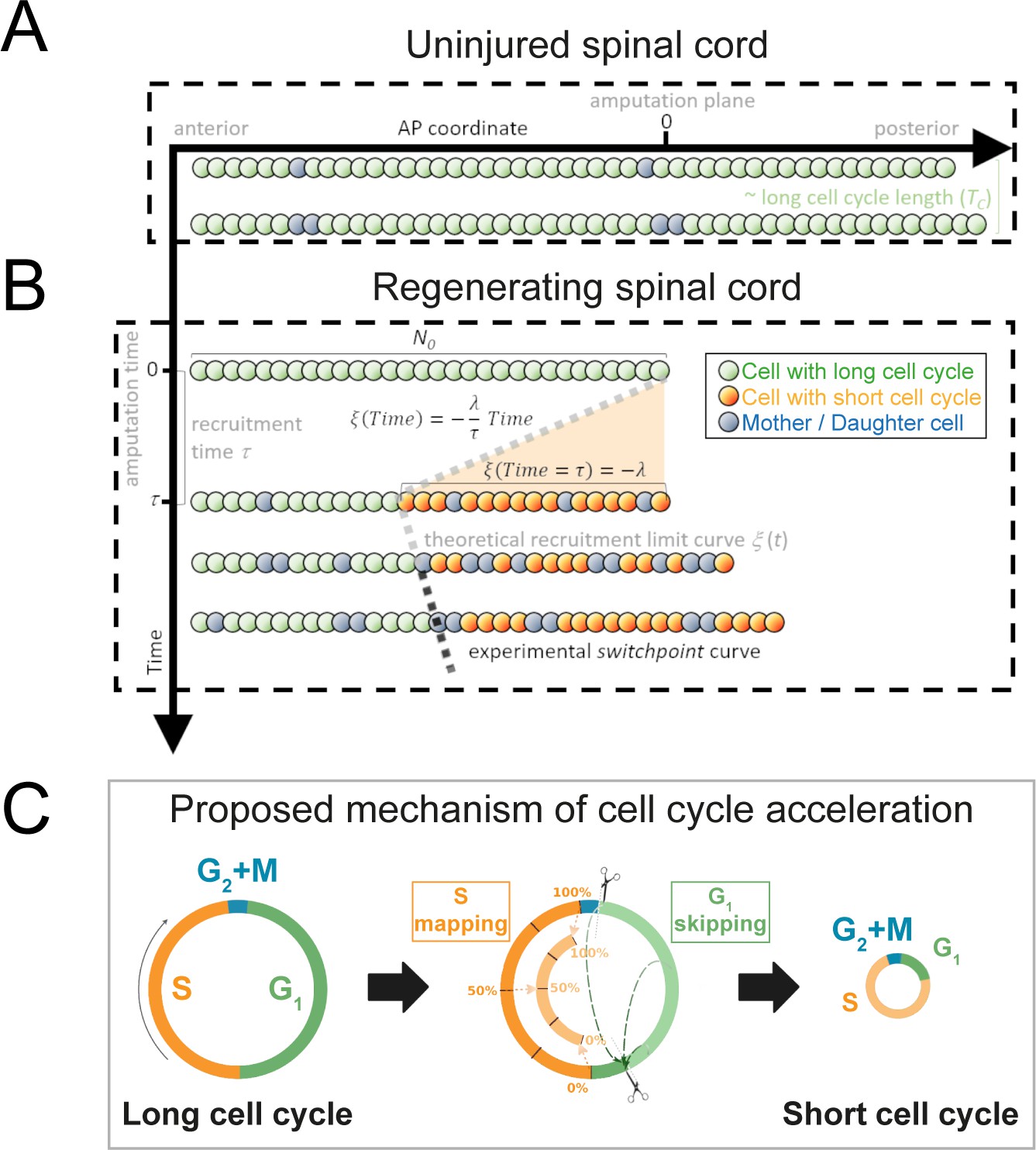
Model of uninjured and regenerating spinal cord growth based on shortening G1 and S phases.
(A) Uninjured spinal cord. 1D model of ependymal cells aligned along the anterior-posterior (AP) axis. In uninjured tissue, ependymal cells cycle with a long cell cycle length (see Figure 1—figure supplement 1). When they divide, they ‘push’ cells posteriorly and the spinal cord tissue grows. As an example, two mother cells (in blue) in the top row give rise to four daughter cells in the second row (also in blue) following one division. This results in a growth of two cell diameters within a timeframe of approximately one long cell cycle length. (B) Regenerating spinal cord. After amputation (AP coordinate and time equal to zero), a signal is released anteriorly from the amputation plane during a time τ and spreads while recruiting resident ependymal cells up to the theoretical recruitment limit ξ located at –λ μm from the amputation plane. After a certain time, the recruitment limit ξ overlaps the experimental switchpoint (see definition of the experimental switchpoint in Figure 1—figure supplement 1). (C) Proposed mechanism of cell cycle acceleration, consisting of partial skipping of G1 phase and proportional mapping between long and short S phases. In the middle panel, two examples are depicted (dashed green arrows) of cells that were in the long G1 phase (immediately before recruitment) that become synchronized (immediately after recruitment). Additionally, there are three examples (dotted orange arrows) of cells that were in the long S phase (immediately before recruitment) that are proportionally mapped (immediately after recruitment). All these examples are shown in detail in Figure 1—figure supplement 2. The diameter of the circles is approximately proportional to the length of the cell’s cell cycle.
Figure 1—figure supplement 1

Space-time distribution of cell proliferation during axolotl spinal cord regeneration.
Experimental switchpoint (black dots) separating areas of low cell proliferation (long cell cycle zone, dark green) from high cell proliferation (short cell cycle zone, light green) along the anterior-posterior axis (depicted horizontally) of the axolotl spinal cord. The dashed region marks the space outside of the spinal cord while the dotted region marks the unaffected part of the spinal cord (adapted from Figure 2F" of Rost et al., 2016). Each switchpoint value was determined as the border separating two spatially homogeneous zones assumed by a mathematical model, which was fitted to the experimental spatial distribution of growth fraction and mitotic index along the axolotl spinal cords (Rost et al., 2016).
Figure 1—figure supplement 2

Further explanation of the cell cycle coordinate transformation invoked by the model.
Cells in G1 phase at the moment of recruitment can skip the remainder of the phase, depending on where they are located in the long G1 phase. If their cell cycle coordinate is before the difference between the long and the short G1 phases, they skip this initial part of the long G1 phase and synchronize at the beginning of the short G1 phase (1, 2). If their cell cycle coordinate is equal or after the difference between the long and the short G1 phases, they continue cycling as before, but they will go through a short S phase afterwards (3). This generates a partial synchronization mechanism (see Section 1.1.1). If the cells are in S phase at the moment of recruitment, cells follow a proportional mapping (4 – 4). Essentially the cell cycle coordinates within S are scaled into the short S phase (see Section 1.1.2).
Figure 2 with 4 supplements
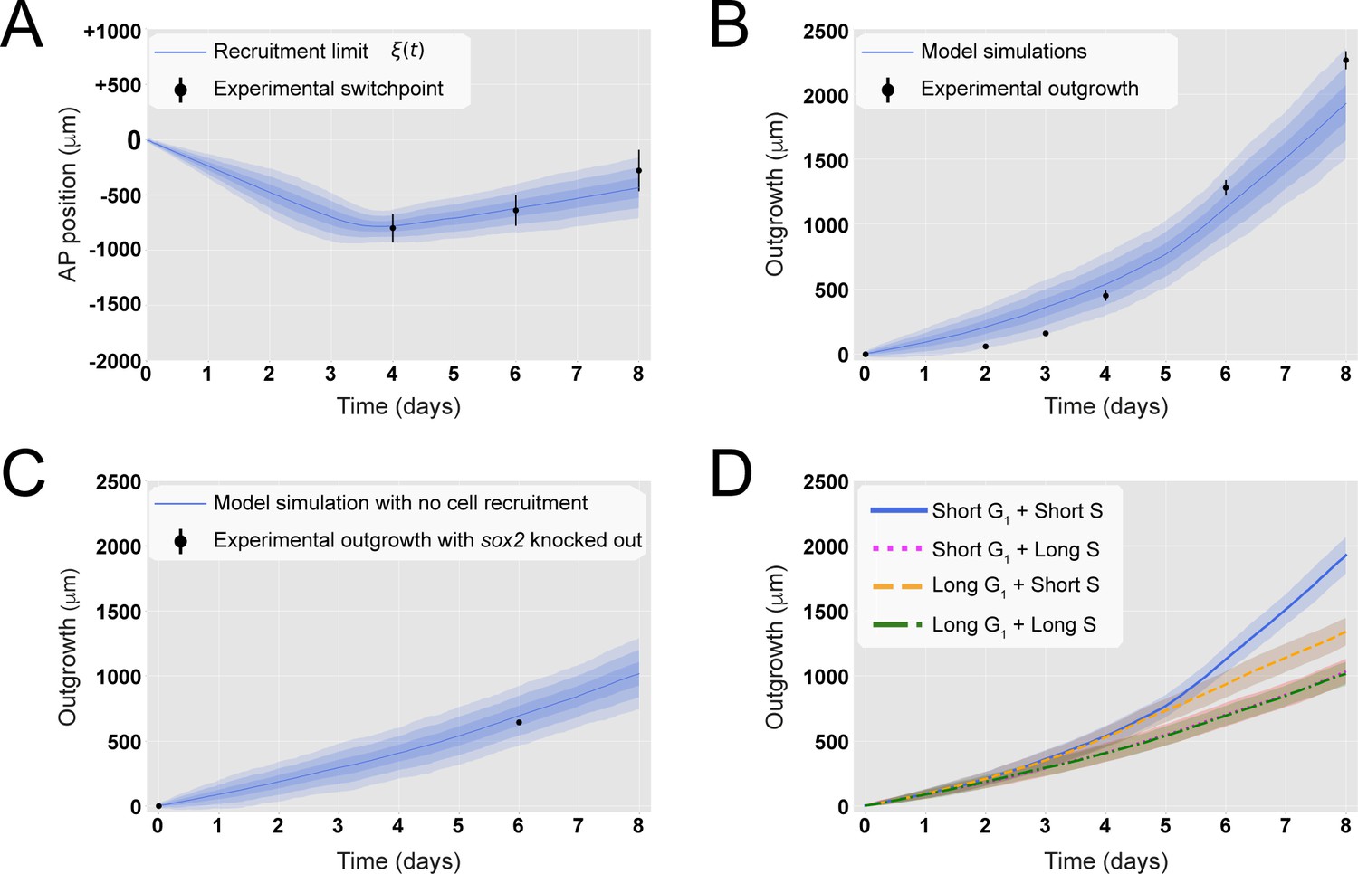
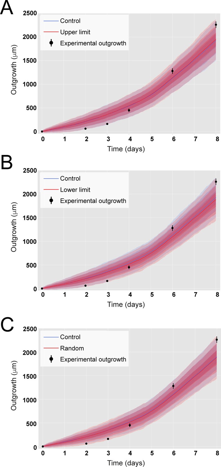
A hypothetical signal recruits ependymal cells up to 828 ± 30 μm anterior to the amputation plane during the 85 ± 12 hours following amputation, recapitulating in vivo spinal cord regenerative outgrowth.
(A) The modeled recruitment limit successfully fits the experimental switchpoint curve. Best-fitting simulations of the model-predicted recruitment limit ξ(t) overlap the experimental switchpoint curve (see definition of the experimental switchpoint in Figure 1—figure supplement 1). Best-fitting parameters are N0 = 196 ± 2 cells, λ = 828 ± 30 μm, and τ = 85 ± 12 hours. (B) The model quantitatively matches experimental axolotl spinal cord outgrowth kinetics (Rost et al., 2016). (C) The model reproduces experimental outgrowth reduction when the acceleration of cell proliferation is impeded. Prediction of the model assuming that neither S nor G1 phase lengths were shortened superimposed with experimental outgrowth kinetics in which acceleration of the cell cycle was prevented by knocking out Sox2 (Fei et al., 2014). Lines in (A–C) show the means while blue shaded areas correspond to 68, 95%, and 99.7% confidence intervals, from darker to lighter, calculated from the 1000 best-fitting simulations. (D) S phase shortening dominates cell cycle acceleration during axolotl spinal cord regeneration. Spinal cord outgrowth kinetics predicted by the model assuming shortening of S and G1 phases (blue line), only shortening of S phase (orange dashed line), only shortening of G1 phase (magenta dotted line), and neither S nor G1 shortening (green line). The magenta line and green line are overlapped with one another. Means are represented as lines, and each shaded area corresponds to 1 sigma out of 1000 simulations.
Figure 2—figure supplement 1
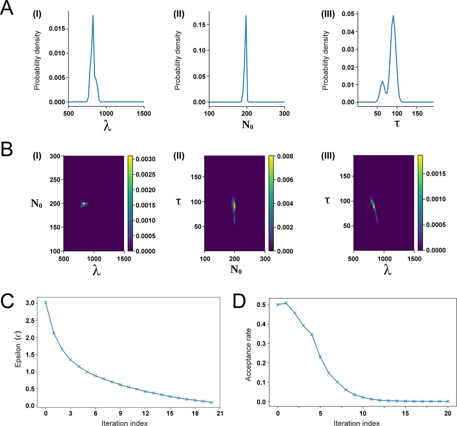
Approximate Bayesian Computation (ABC) fitting of the recruitment limit model to the experimental switchpoint data.
(A) Posterior distributions of the parameters λ (I), N0 (II), and τ (III). (B) Combined posterior distributions of N0 and λ (I), τ and N0 (II), as well as τ and λ (III). (C, D) Fitting process convergence depicted by the fitting tolerance ε (B) and the acceptance rate (D) versus the iteration index (see Section 1.3 for details).
Figure 2—figure supplement 2
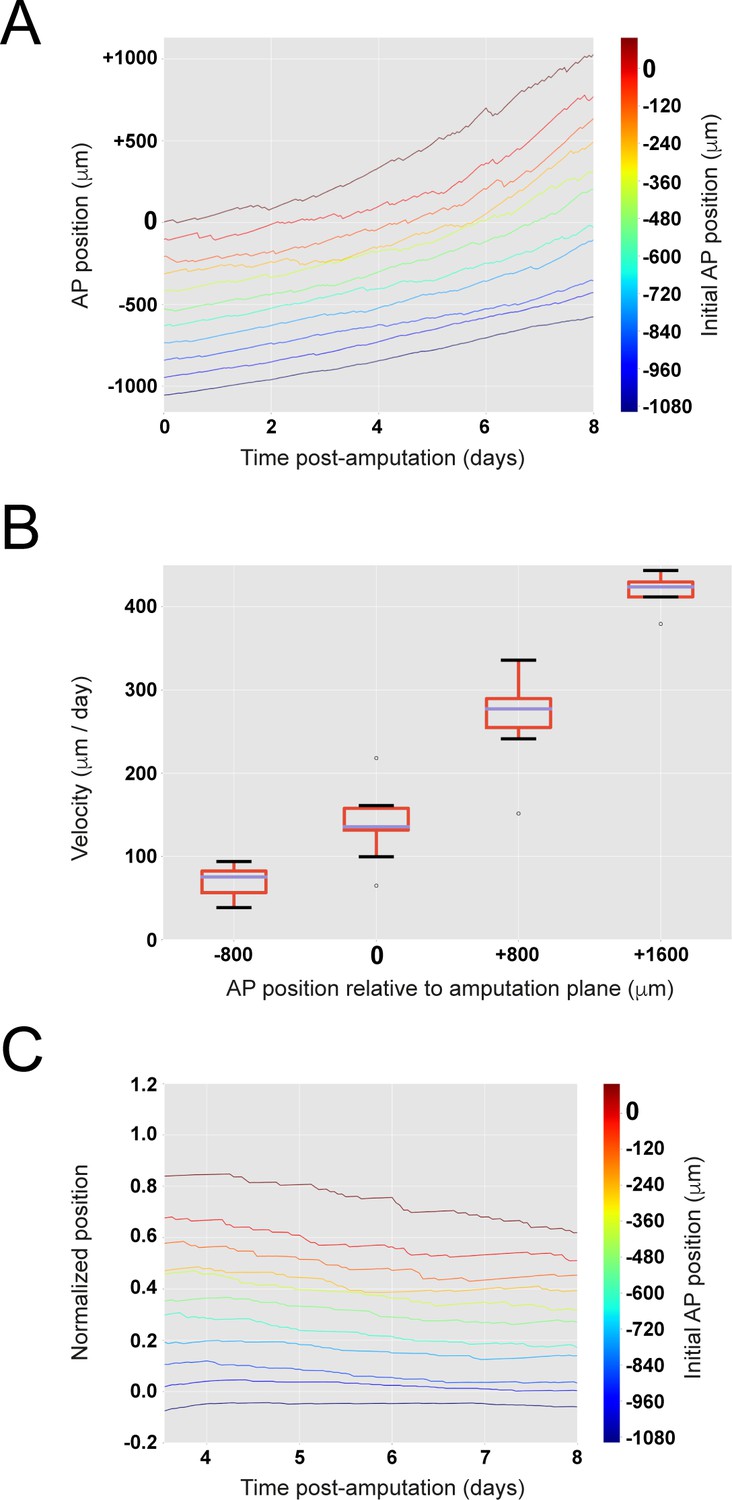
The model encompasses the cell pushing mechanism: the more posterior a cell is, the faster it moves.
(A) Cells located close to the amputation plane end up at the posterior end of the regenerated modeled tissue. (B) Clone velocity monotonically increases with anterior-posterior coordinate. Box plot representation showing median of clone velocities binned every 800 μm. (C) Scaling behavior: clone cells preserve their original spatial order. Relative position of each clone to the highly proliferating tissue delimited by its outgrowth and the recruitment limit remains constant in time. The figure depicts 11 simulations.
Figure 2—figure supplement 3
Incorporating variability of cell length along the anterior-posterior (AP) axis does not impact on predicted axolotl spinal cord outgrowth.
(A) Outgrowth predicted from the model assuming ependymal cell lengths equal to the experimental mean value plus 3 sigma of their cell length measured along the AP axis (in red). (B) Outgrowth predicted from the model assuming ependymal cell lengths equal to the experimental mean value minus 3 sigma of their cell length measured along the AP axis (in red). (C) Outgrowth predicted from the model assuming ependymal cell lengths extracted from a normal distribution parametrized from the experimental cell length measured along the AP axis (in red). In the three panels, it is depicted the outgrowth predicted from the model assuming ependymal cell lengths equal to the experimental mean value of their cell length measured along the AP axis (Control, in blue, same simulations shown in Figure 2B). Experimental ependymal cell lengths along the AP axis are characterized by μ = 13.2 μm, σ = 0.1 μm.
Figure 2—figure supplement 4
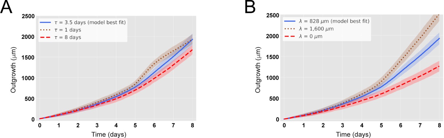
The maximal recruitment time (τ) and the maximal recruitment length (λ) determine the outgrowth of the axolotl spinal cord.
(A) Increase (decrease) of τ reduces (increases) the model-predicted spinal cord outgrowth. Time course of spinal cord outgrowth predicted by the model when varying τ from 1 day (brown) to 8 days (red). In blue, the prediction of the model assuming τ = 85 ± 12 hours. N0 = 196 ± 2 cells and λ = 828 ± 30 μm. (B) Increase (decrease) of λ increases (reduces) the model-predicted spinal cord outgrowth. Time course of spinal cord outgrowth predicted by the model when varying λ from 0 (red) to 1600 μm (brown). In blue, the prediction of the model assuming λ = 828 ± 30 μm. N0 = 196 ± 2 cells and τ = 85 ± 12 hours. Simulations depicted in the blue curves in (A) and (B) are the same simulations shown in Figure 2B. Means are depicted as lines while shaded areas correspond to 68% confidence intervals, respectively, calculated from 1000 simulations.
Figure 3 with 5 supplements

AxFUCCI – a transgenic cell cycle reporter for axolotl.
(A) Top panel: AxFUCCI design. A ubiquitous promoter (CAGGs) drives expression of two AxFUCCI probes (AxCdt1[1-128]-Venus and mCherry-AxGmnn[1-93]) in one transcript. The two AxFUCCI probes are separated co-translationally by virtue of the viral ‘self-cleaving’ T2A peptide sequence. Bottom panel: AxFUCCI fluorescence combinations in each phase of the cell cycle. (B) Live imaging of a single AxFUCCI-electroporated axolotl cell in vitro. Each panel is a single frame acquired at the indicated hour (h) after the start of the imaging session. One cell cycle (from S/G2 to the subsequent S/G2) is depicted. At 67 hours, the two mitotic daughter cells moved apart; the asterisked daughter cell is depicted in the remaining panels. (C) Establishment of AxFUCCI transgenic axolotls. The location of the spinal cord is indicated in the context of the tail. (D) A fixed AxFUCCI tail, cleared and imaged in wholemount using lightsheet microscopy. The 3D data enable post-hoc digital sectioning of the same spinal cord into lateral, dorsal, or transverse views. Images depict maximum intensity projections through 50 μm (lateral and transverse views) or 150 μm (dorsal view) of tissue. Trans.: Transition-AxFUCCI (G1/S or G2/M transition).
Figure 3—figure supplement 1
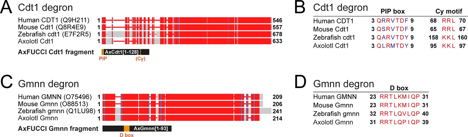
Determination of Cdt1 and Gmnn fragments for AxFUCCI reporter.
(A) Alignment of full-length Cdt1 proteins from human, mouse, zebrafish, and axolotl. Uniprot identifiers are given in parentheses. Numbers indicate amino acid residue numbers. Red regions indicate high amino acid similarity/identity; gray regions indicate low conservation. Alignments were performed using COBALT (NCBI). The AxFUCCI Cdt1 fragment comprises amino acids 1–128 of axolotl Cdt1, harboring the PIP box degron and corresponding to amino acids 1–190 of zebrafish cdt1 used to make zebrafish FUCCI (Sugiyama et al., 2009; Bouldin et al., 2014). (B) Amino acid alignments at the Cdt1 degron sequences. The PIP box is well conserved evolutionarily. Like zebrafish cdt1, axolotl Cdt1 harbors a ‘KKL’ motif rather than the ‘RRL’ motif found in human and mouse. (C) Alignment of full-length Gmnn proteins from human, mouse, zebrafish, and axolotl. The AxFUCCI Gmnn fragment comprises amino acids 1–93 of axolotl Gmnn, harboring the Destruction (D) box and corresponding to amino acids 1–100 of zebrafish gmnn1 used to make zebrafish FUCCI (Sugiyama et al., 2009; Bouldin et al., 2014). (D) Amino acid alignments at the Gmnn D box.
Figure 3—figure supplement 2
Fluorescence intensity measurements of AxFUCCI through the cell cycle.
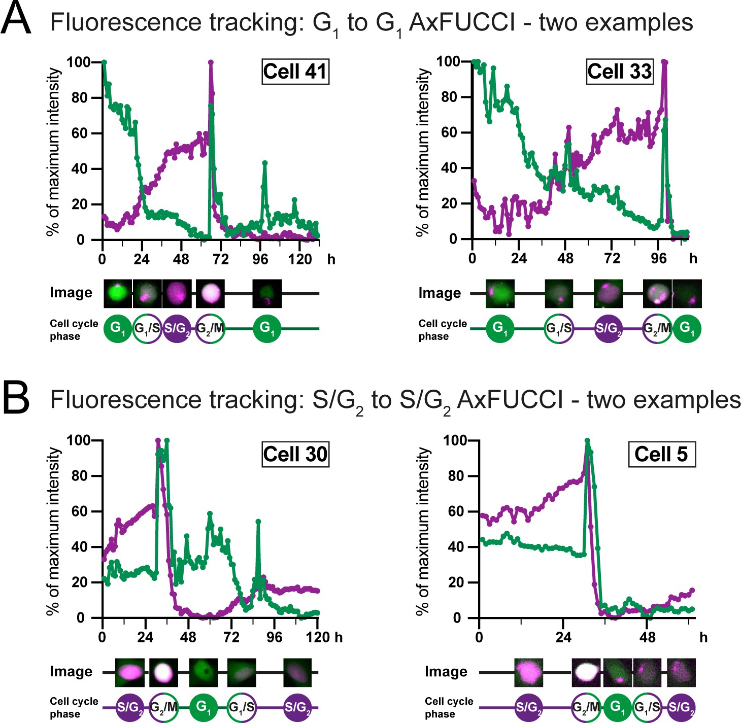
Fluorescence intensity measurements of AxFUCCI-electroporated AL1 cells as they transited through one cell cycle from G1 to the following G1 (A) or S/G2 to the following S/G2 (B). Two examples are presented for each transition. Green lines represent G0/G1-AxFUCCI fluorescence; magenta lines represent S/G2-AxFUCCI fluorescence. For each time point, the cell nucleus was segmented and the mean fluorescence intensity calculated. Fluorescence intensities were normalized to the maximal fluorescence value observed during the imaging session. h: hours after start of imaging. Maximum fluorescence is observed at mitosis when the cell rounds up in preparation for cell division. Mean fluorescence intensity decreases sharply after each mitosis due to fluorophore and plasmid dilution between the two daughter cells. For sample videos, see Video 2 and Video 3.
Figure 3—figure supplement 3

DNA quantification by flow cytometry to validate AxFUCCI functionality.
Relative DNA content in G0/G1-AxFUCCI (green), S/G2-AxFUCCI (magenta), or Transition-AxFUCCI (gray) cells. AxFUCCI-electroporated AL1 cells were incubated with Hoechst DNA stain-containing cell culture medium for 90 min prior to dissociation and analysis.
Figure 3—figure supplement 4
Validation of AxFUCCI functionality through in vivo tissue analysis.
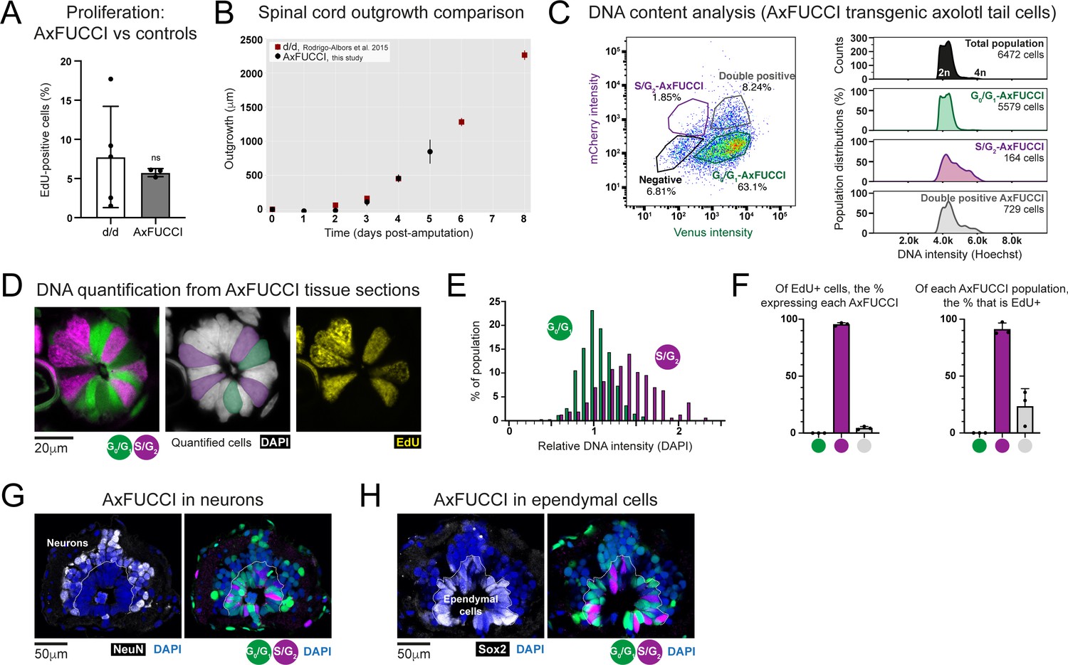
(A) Baseline proliferation in AxFUCCI spinal cord is not significantly different from d/d controls. EdU was administered in a 2 hours pulse to uninjured AxFUCCI or d/d control animals. Tails were harvested and sectioned to quantify EdU-labeled proliferative cells in the spinal cord. ns: not significant, p=0.62 (two-sample t-test). Error bars indicate standard deviation. n = 5 tails (control) or three tails (AxFUCCI), 750 cells counted in total for each, of which ~50 cells were EdU-labeled. (B) AxFUCCI tails regenerate with normal kinetics. Spinal cord outgrowth was measured every day up to 5 days after AxFUCCI tail amputation and plotted together with measurements previously obtained from d/d control animals (Rodrigo Albors et al., 2015). See Section 2.11 for details of how spinal cord outgrowth was measured. (C) DNA quantification by flow cytometry. Relative DNA content in G0/G1-AxFUCCI (green), S/G2-AxFUCCI (magenta), or Transition-AxFUCCI (gray) cells dissociated and harvested from uninjured AxFUCCI axolotl tails. Cells were incubated with Hoechst DNA stain for 60 min prior to analysis. (D) DNA quantification from AxFUCCI tissue sections. Single-section confocal image of a 10 μm-thick AxFUCCI spinal cord cross-section, co-stained with DAPI (gray) to label DNA. The DNA intensity of G0/G1-AxFUCCI cells (green) was compared to that of S/G2-AxFUCCI cells (magenta). The center panel depicts the cells that satisfy the criteria for quantification – they must span the spinal cord, contact the lumen, and not be obscured by neighboring cells. The AxFUCCI animals were also pulsed with EdU for 8 hours prior to tail harvesting. S/G2-AxFUCCI cells, but not G0/G1-AxFUCCI cells, incorporated EdU (yellow, right panel). (E) Histogram depicting the DAPI intensities of AxFUCCI cells quantified in (D). The mean intensity of G0/G1-AxFUCCI cells was set to an arbitrary value of 1 (2n). S/G2-AxFUCCI cells have a significantly higher DNA content than G0/G1-AxFUCCI cells (P = 2.20 × 10⁻¹⁶, Welch’s test). n = 3 tails (a total of 341 G0/G1-AxFUCCI cells vs. 157 S/G2-AxFUCCI cells). (F) Correlation of EdU labeling (see panel D) with each AxFUCCI-expressing population. n = 3 tails, 819 AxFUCCI-expressing cells were counted in total, of which 171 had incorporated EdU. (G) Spinal cord neurons express G0/G1-AxFUCCI. NeuN-expressing neurons are located on the periphery of the spinal cord. 98% ± 1.5% of neurons expressed G0/G1-AxFUCCI, and the remainder did not express any AxFUCCI. n = 5 tails, a total of 2,170 NeuN+ cells counted. (H) Ependymal cells express all AxFUCCI combinations. Sox2-expressing ependymal cells are located on the interior of the spinal cord, lining the lumen.
Figure 3—figure supplement 5
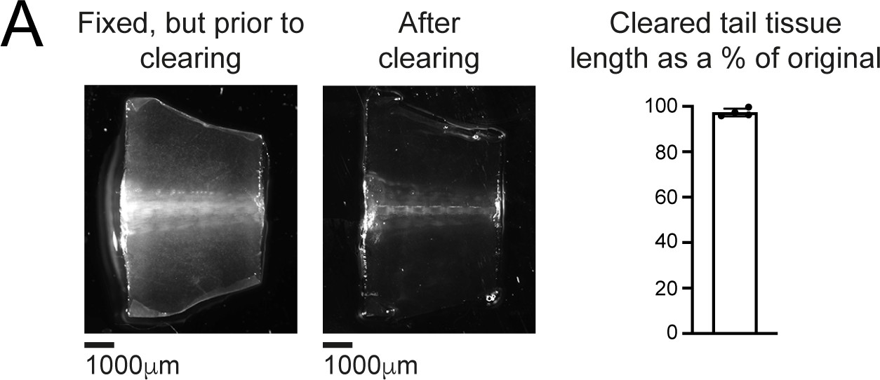
The tissue clearing protocol does not alter spinal cord length.
The same, fixed tail tissue imaged prior to (left) or following (center) tissue clearing and refractive index matching. Right: cleared tail tissue preserves 97% ± 1.7% of its length compared to uncleared tail tissue. n = 3 tails.
Figure 4 with 2 supplements
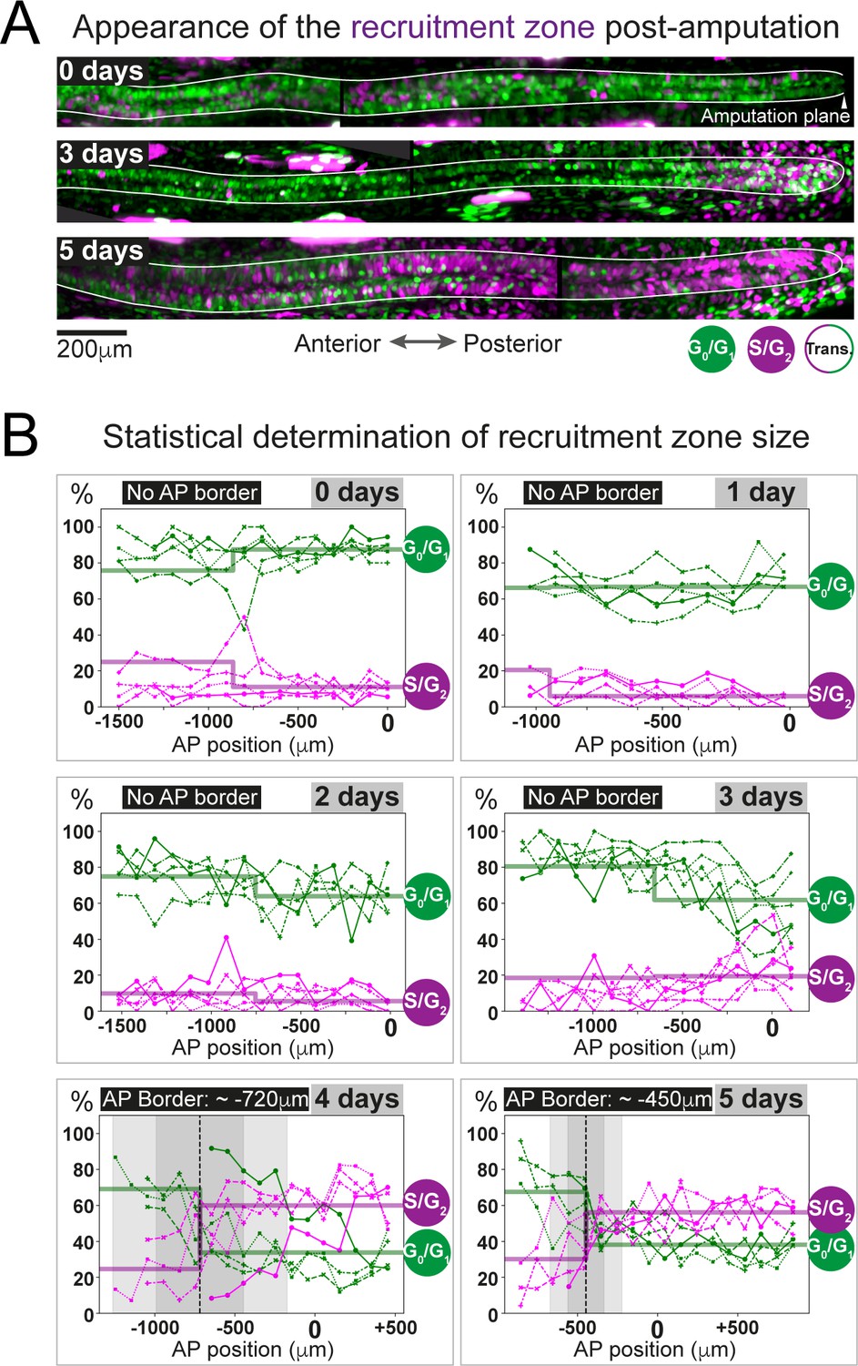
The predicted recruitment zone size is observed in AxFUCCI tails after amputation.
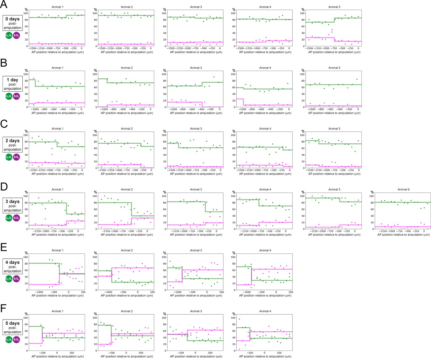
(A) Visualization of the recruitment zone in AxFUCCI tails. At amputation, most ependymal cells are G0/G1-AxFUCCI positive (green). After amputation, a decrease in G0/G1-AxFUCCI and an increase in S/G2-AxFUCCI (magenta) expression is seen anterior to the amputation plane, and this zone increases in size anteriorly through day 5 post-amputation. The spinal cord is outlined. Images depict maximum intensity projections through 30 μm of tissue and are composites of two adjacent fields of view. (B) Quantification of the anterior-posterior border (AP border) that delimits the recruitment zone in G0/G1 and S/G2-AxFUCCI data. Percentage of G0/G1 (in green) and S/G2 (in magenta)-AxFUCCI-expressing cells quantified in 100 μm bins along the AP spinal cord axis. A mathematical model assuming two adjacent spatially homogeneous zones separated by an AP border was fitted to the G0/G1 and S/G2-AxFUCCI-data for each animal. Significant differences between anterior and posterior zones were detected only at days 4 and 5 (Kolmogorov–Smirnov test p=0.0286). The AP border mean and 2 sigmas are depicted as a black dashed line and a gray shaded areas, respectively. AP position is defined with respect to the amputation plane (0 μm). n = 4–6 tails per time point, ~300 cells each. Different symbols depict different animals; each line represents one animal. Best-fitting values of the model regarding the anterior and posterior percentage of AxFUCCI data are in Figure 4—figure supplement 1. Individual fittings are in Figure 4—figure supplement 2. For more details, see Section 2.12.
Figure 4—figure supplement 1
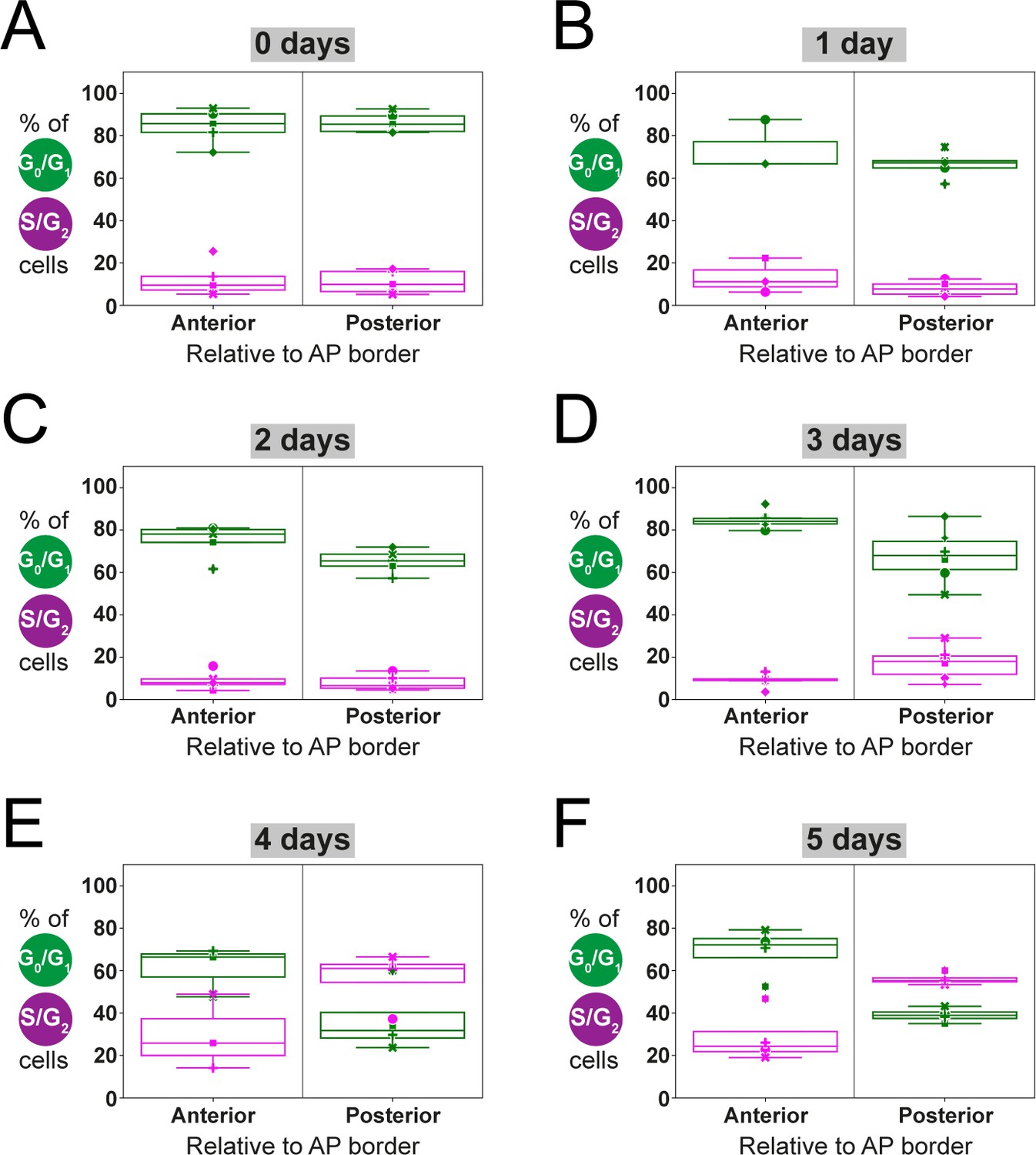
Estimation of anterior and posterior (AP) percentages of G0/G1-AxFUCCI and S/G2-AxFUCCI-expressing cells by fitting a two-zones model.
Dots correspond to the best-fitting value of the parameters , and to the experimental spatial AP profiles of the percentages of G0/G1-AxFUCCI (in green) and S/G2-AxFUCCI (in magenta) expressing cells for each animal, at each time point. (A–E) Each symbol identifies a different animal (same criteria as in Figure 4). Box plots show that at 0–3 days post-amputation, AP values are not significantly different from each other (A–D). In contrast, at days 4 and 5, AP values are significantly different (E, F) (Kolmogorov–Smirnov test p=0.0286) (see Section 2.12 for more details).
Figure 4—figure supplement 2
Individual fitting of the two-zones model to experimental AP profiles of the percentages of G0/G1-AxFUCCI and S/G2-AxFUCCI-expressing cells.
Percentage of G0/G1 (in green) and S/G2 (in magenta)-AxFUCCI-expressing cells quantified in 100 μm bins along the AP spinal cord axis. A mathematical model assuming two adjacent spatially homogeneous zones separated by an AP border was fitted to the G0/G1 and S/G2-AxFUCCI-data for each animal at time 0 (A), 1 (B), 2 (C), 3 (D), 4 (E), and 5 (F) days post-amputation. AP position is defined with respect to the amputation plane (0 μm). Best-fitting values of the model regarding the AP percentage of AxFUCCI data are in Figure 4—figure supplement 1 (for more details, see Section 2.12).
Figure 5 with 1 supplement
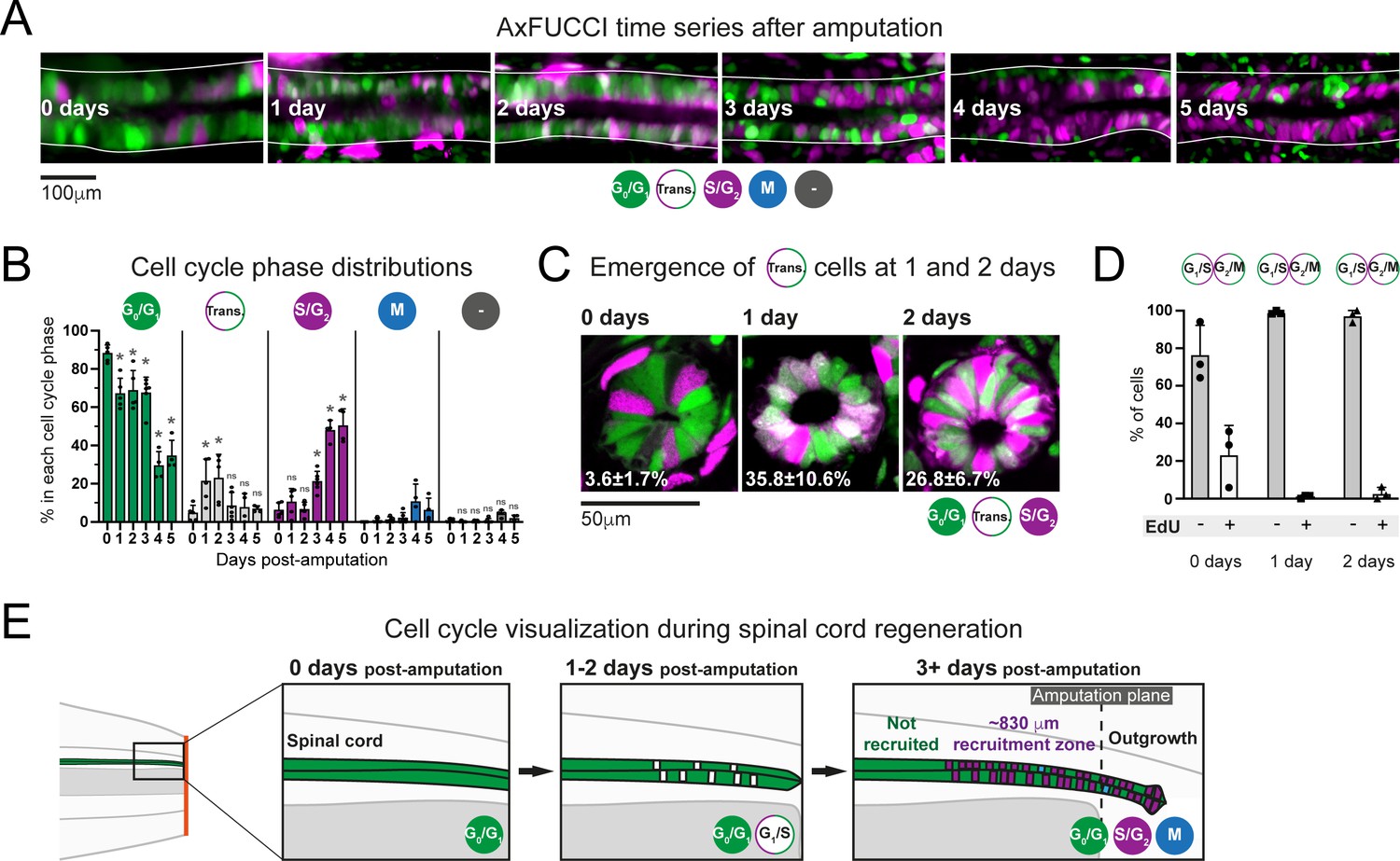
Ependymal cells exhibit cell cycle synchrony during spinal cord regeneration.
(A) Cell cycle distributions of ependymal cells during the first 5 days of regeneration. Maximum intensity projections through 25 μm of spinal cord oriented anterior to left and posterior to right. The spinal cord is outlined. The lumen is in the center. Images were taken from within the 600 μm of most posterior regenerating spinal cord. (B) AxFUCCI data separated by cell cycle phase. Percentage of ependymal cells in each cell cycle phase in the 600 μm of most posterior regenerating spinal cord between 0 and 5 days post-amputation. Cells in mitosis (M) were counted independently of AxFUCCI and were identified based on their condensed chromatin as revealed by staining with DAPI (not shown). The percentage of AxFUCCI-negative cells (‘-‘) was negligible and did not change at any time point (p=0.40, Wilcoxon rank sum). Each dot represents data from one tail. n = 4–6 tails per time point, ~100 cells each. Error bars indicate standard deviations. Day 0 data (immediately after amputation) were taken as baselines, and statistical analyses were performed against these baselines. Kruskal–Wallis tests followed by Wilcoxon rank sum tests revealed a significant decrease in G0/G1-AxFUCCI from 1 day post-amputation (p=0.02) and a significant increase in S/G2-AxFUCCI starting at 3 days post-amputation (p=0.02). One-way ANOVA followed by Tukey’s HSD test revealed a significant increase in Transition-AxFUCCI cells at 1 and 2 days post-amputation (p=0.04 and 0.02, respectively), but not at later days post-amputation (p>0.99). Mitotic cells were absent in the 0 day samples, precluding statistical analysis. ns: not statistically significant. (C) The emergence of Transition-AxFUCCI cells at 1 and 2 days post-amputation was confirmed in tissue sections. Images are single-plane confocal images of spinal cord cross-sections fixed at the indicated times after amputation. Percentages indicate the percentage of Transition-AxFUCCI cells at each time point (mean ± standard deviation). n = 3 tails per time point, ~400 cells counted in each, corresponding to ~750 μm of spinal cord. (D) Transition-AxFUCCI-expressing cells at 1 and 2 days post-amputation reside at the G1/S transition. Transition-AxFUCCI cells can be either at the G1/S transition or the G2/M transition. Following an 8 hours (0 days) or 24 hours (1 and 2 days) EdU pulse, only G2/M cells should become labeled with EdU. Tails were fixed, then processed for tissue sectioning and EdU detection. >97% of Transition-AxFUCCI cells were EdU-negative at 1 and 2 days post-amputation, indicating that they reside at the G1/S transition. n = 3 tails per time point. A total of 36, 442, and 315 Transition-AxFUCCI cells were assayed at 0, 1, and 2 days post-amputation, respectively. (E) Cell cycle dynamics during axolotl spinal cord regeneration.
Figure 5—figure supplement 1
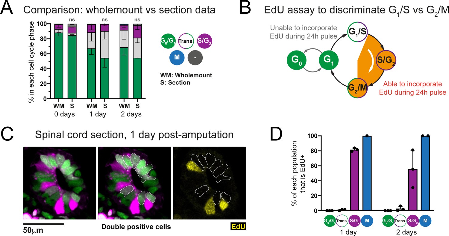
Transition-AxFUCCI cells at 1 and 2 days post-amputation reside at the G1/S boundary.
(A) Comparison of AxFUCCI quantifications made from wholemount specimens (Whole) or tissue sections (Section). No difference was observed between wholemount-based quantifications and section-based quantifications (one-way ANOVA). n = 3 tails per time point, ~400 cells counted in each, corresponding to ~750 μm of spinal cord. Error bars indicate standard deviation. (B) EdU-based assay to distinguish G1/S cells and G2/M cells. (C) Single confocal image of a spinal cord at 1 day post-amputation, pulsed for 24 hours with EdU prior to harvesting. Transition-AxFUCCI cells (double positive, outlined) have not incorporated EdU (yellow). Neighboring S/G2-AxFUCCI cells (magenta) have incorporated EdU (internal control). (D) The percentage of each AxFUCCI population and mitotic cells that incorporated EdU in the assay in (B). As expected, no G0/G1-AxFUCCI cells incorporated EdU and all mitotic cells had incorporated EdU. The majority of S/G2-AxFUCCI cells had incorporated EdU. In contrast, almost none of the Transition-AxFUCCI cells at 1 and 2 days post-amputation incorporated EdU, indicating that they reside at the G1/S transition. n = 3 tails per time point. Total cells counted per time point: 1 day post-amputation (671 G0/G1-AxFUCCI, 115 S/G2-AxFUCCI, 442 Transition-AxFUCCI, 1 mitotic cell), 2 days post-amputation (643 G0/G1-AxFUCCI, 191 S/G2-AxFUCCI, 315 Transition-AxFUCCI, 3 mitotic cells).
Figure 6 with 2 supplements
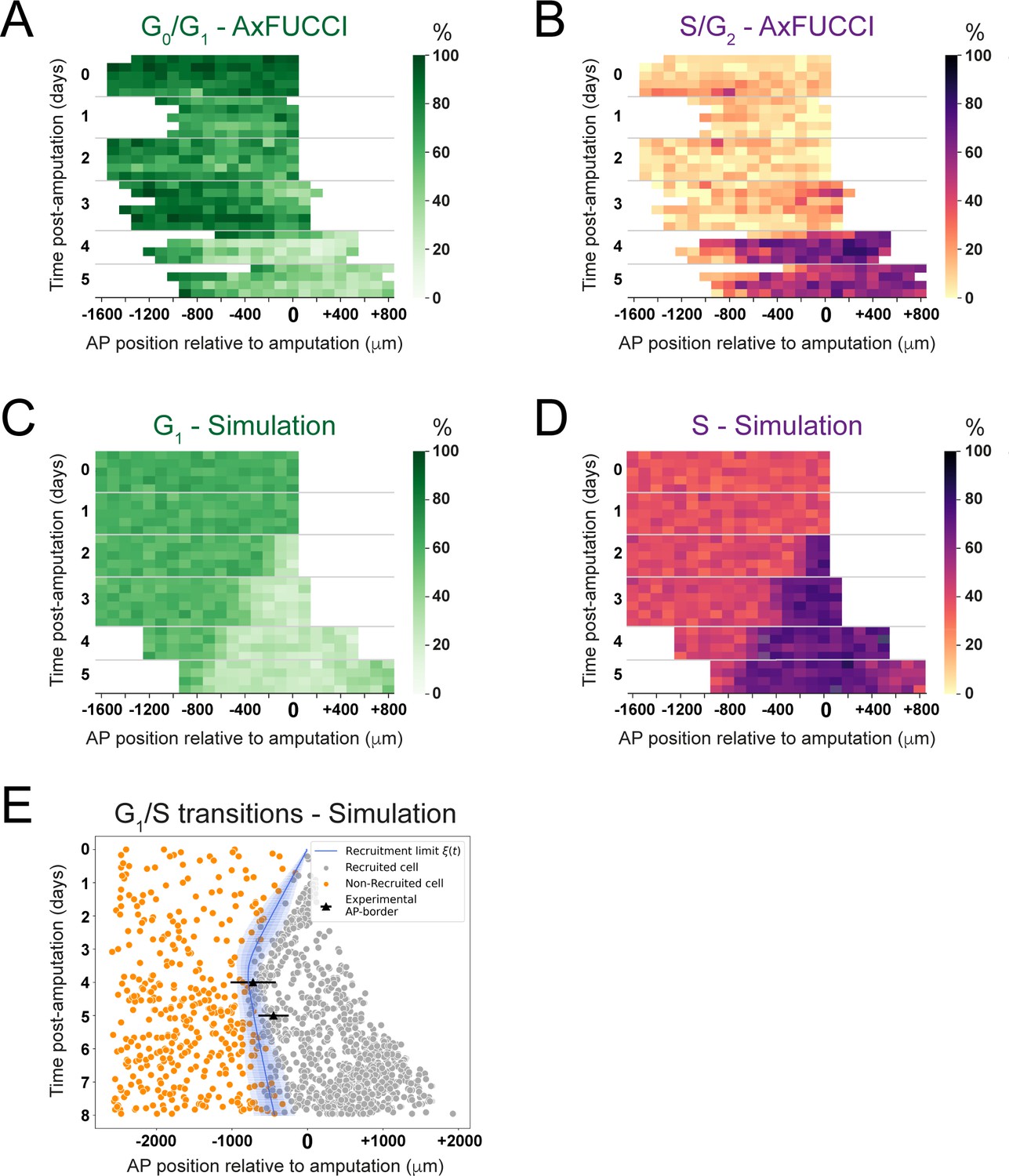
Convergence of cell cycle response between the model simulations and the AxFUCCI data.
Heatmaps depicting spatiotemporal distribution of G0/G1-AxFUCCI cells (A), S/G2-AxFUCCI cells (B), model-predicted cells in G1 phase (C), and model-predicted cells in S phase (D). x-axes depict anterior-posterior (AP) position with respect to the amputation plane (AP position = 0 μm). y-axes depict time (days) post-amputation and both experimental and simulated replicates within each time point. The color codes correspond to the percentage of cells in the corresponding phase. Transition-AxFUCCI data are in Figure 6—figure supplement 2. (E) Model-predicted occurrence of G1-S transitions is more often within the recruited cells (gray circles) compared to the non-recruited (orange crosses) cells. At days 4 and 5, the recruitment limits overlap with the AP borders. Independent simulations from 10 independent seeds are shown and the model is parameterized as in Figure 2.
Figure 6—figure supplement 1
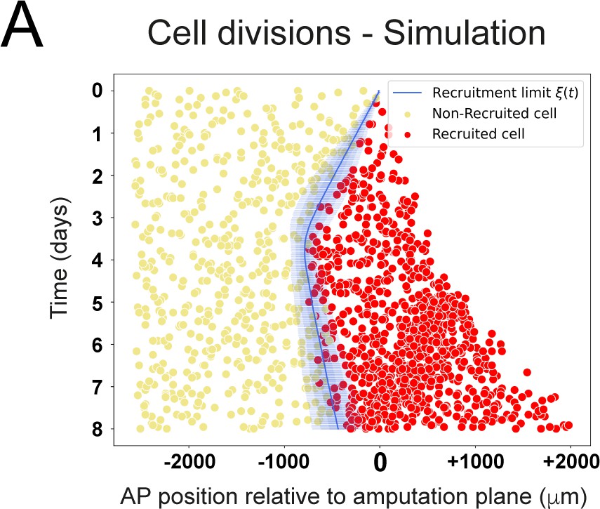
Modeled spatiotemporal distributions of ependymal cell divisions during axolotl spinal cord regeneration.
Model-predicted occurrence of cell divisions is more often within the recruited (red crosses) compared to the non-recruited (yellow circles) cells, where recruited and non-recruited cells are separated by the recruitment limit ξ(t). The model is parameterized as in Figure 2 and Figure 6C,D,E.
Figure 6—figure supplement 2
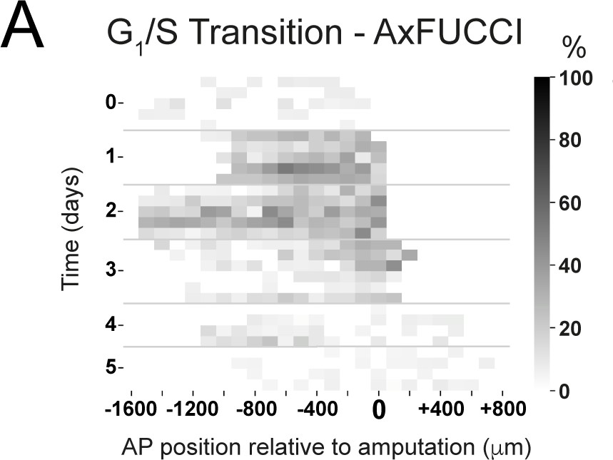
Spatiotemporal distributions of Transition-AxFUCCI cells during axolotl spinal cord regeneration.
Heatmaps depicting experimental spatiotemporal distribution of Transition-AxFUCCI cells. Anterior-posterior (AP) position is depicted horizontally with respect to the amputation plane (AP position = 0 μm). In the vertical axis, time from amputation (Time = 0 days) and experimental replicates within each time. The color code corresponds to the percentage of Transition-AxFUCCI cells. The increase in Transition-AxFUCCI cells at days 1 and 2 post-amputation is readily observed.
Videos
Video 1
1D model simulations of spinal cord regeneration.
(Top panel) 20 model simulations from 20 different random seeds (the seeds are shown in the vertical axis). The color code corresponds to the generation of each cell (blue, orange and black correspond to the first, second and third generation, respectively). Vertical interrupted black line denotes the amputation plane (AP coordinate of 0). The recruitment limit ξ(t) (vertical red dashed line) propagates linearly in time up until the time t of 85 hours post amputation, covering up the maximal recruitment λ of 828 mm anterior to the amputation plane. (Bottom left panel) Predicted recruitment limit ξ(t) as a function of time from the simulations showed in the top panel. Mean value is depicted in the red line while the red shaded areas corresponds to 68, 95 and 99.7 % confidence intervals (Bottom right panel) Predicted spinal cord outgrowth predicted by the model from the simulations showed in the top paneladapte. The line represents to the mean (also indicated as the blue vertical line in the top panel) and the blue shaded areas correspond to the 68, 95 and 99.7 % confidence intervals. The 20 simulations have the same parametrization than the 1,000 simulations showed in Figure 2A and B.
Video 2
Live imaging of an AxFUCCI-electroporated AL1 cell (G1 to G1).
A single AxFUCCI-electroporated AL1 cell passing through one cell cycle from G1 to G1, imaged hourly over ~130h. The cell transitions through the cell cycle phases in the following order: Green (G0/G1-AxFUCCI) > White (Transition-AxFUCCI) > Magenta (S/G2-AxFUCCI) > White (Transition-AxFUCCI) > Mitosis > Two Green daughter cells (G0/G1-AxFUCCI). This cell corresponds to Cell 41 tracked in Figure 3—figure supplement 2. Fluorescence intensity drops after mitosis due to fluorophore and plasmid dilution (non-integrating transgene).
Video 3
Live imaging of an AxFUCCI-electroporated AL1 cell (S/G2 to S/G2).
A single AxFUCCI-electroporated AL1 cell passing through one cell cycle from S/G2 to S/G2, imaged overly over ~120h. The cell transitions through the cell cycle phases in the following order: Magenta (S/G2-AxFUCCI) > White (Transition-AxFUCCI) > Mitosis > Two Green daughter cells (G0/G1-AxFUCCI) > White (Transition-AxFUCCI) > Magenta (S/G2-AxFUCCI). This cell corresponds to Cell 30 tracked in Figure 3—figure supplement 2. Fluorescence intensity drops after mitosis due to fluorophore and plasmid dilution (non-integrating transgene).
Video 4
3D imaging of an optically cleared AxFUCCI tail tip.
Volume rendering of a fixed and optically cleared AxFUCCI tail tip, co-stained for DNA using DAPI (blue) and imaged with a lightsheet microscope. The spinal cord is visible as an intensely green and magenta rod at the center of the sample. Peripheral signal is AxFUCCI expression in surface epidermal cells. Other internal structures, including notochord, have weaker AxFUCCI expression and are not visible in this rendering. Volume rendering was performed using Imaris software. See also Figure 3D.
Video 5
1D Model simulations of spinal cord regeneration showing cells in G1 and S phases.
20 model simulations from 20 different random seeds (the seeds are shown in the vertical axis). Cells in G1 and S are depicted in green and magenta, respectively. Predicted recruitment limit ξ(t) and outgrowth are indicated with the vertical red and blue discontinuous lines, respectively. Amputation plane is depicted as a vertical black dashed line. The simulations have the same parametrization than the simulations showed in Figure 2A and B.
Tables
Table 1
Model parameters.
| Model parameter | Value/explanation | Fixed/free |
|---|---|---|
| G1 phase non-regenerating mean | 152 hours | Fixed parameters, extracted from Rodrigo Albors et al., 2015 |
| G1 phase non-regenerating sigma | 54 hours | |
| S phase non-regenerating mean | 179 hours | |
| S phase non-regenerating sigma | 21 hours | |
| G2 + M phases non-regenerating mean | 9 hours | |
| G2 + M phases non-regenerating sigma | 6 hours | |
| G1 phase regenerating mean | 22 hours | |
| G1 phase regenerating sigma | 19 hours | |
| S phase regenerating mean | 88 hours | |
| S phase regenerating sigma | 9 hours | |
| G2 + M phases regenerating mean | 9 hours | |
| G2 + M phases regenerating sigma | 2 hours | |
| GF non-regenerating | 0.12 | |
| Cell length along the AP axis | 13.2 μm | |
| tG0-G1 | 48 hours | |
| N0 | Initial number of cells along the AP axis, anterior to the amputation plane | Free parameters (determined in this study) |
| λ | Maximal length from the amputation plane recruited by the signal (μm) | |
| τ | Maximal time for cell recruitment (days after amputation or hours after amputation) |
-
GF: growth fraction; AP: anterior-posterior.
Key resources table
| Reagent type (species) or resource | Designation | Source or reference | Identifiers | Additional information |
|---|---|---|---|---|
| Strain, strain background (Ambystoma mexicanum, d/d strain) | Axolotl, d/d strain | Tanaka lab axolotl colony | - | Axolotl stock maintained in Tanaka lab, Vienna, Austria. |
| Genetic reagent (Ambystoma mexicanum, AxFUCCI transgenic) | Transgenic AxFUCCI axolotl | This paper | - | Transgenic stock generated in d/d genetic background in Tanaka lab, Vienna, Austria. |
| Gene (Ambystoma mexicanum) | Cdt1 | Axolotl genome release v6.0-DD Schloissnig, 2021 | CDT1|AMEX60DD201052583.1 | Axolotl genome release v6.0-DD available at: https://www.axolotl-omics.org/assemblies. |
| Gene (Ambystoma mexicanum) | Gmnn | Axolotl genome release v6.0-DD Schloissnig, 2021 | GMNN|AMEX60DD301038574.1 | Axolotl genome release v6.0-DD available at: https://www.axolotl-omics.org/assemblies. |
| Cell line (AL1, Ambystoma mexicanum) | AL1 cells | Roy et al., 2000 | - | AL1 cells were kindly provided by Dr David Gardiner (UC Irvine). AL1 cells are an immortalized mesenchymal axolotl line originally derived from a limb blastema. |
| Recombinant DNA reagent | Addgene plasmid mVenus N1 | Addgene | RRID:Addgene_27793 | To amplify coding sequence for mVenus fluorescent protein by PCR. |
| Recombinant DNA reagent | pAxFUCCI | This paper | pAxFUCCI | Plasmid encoding AxFUCCI. Used to generate AxFUCCI transgenic axolotls by I-SceI-mediated transgenesis. |
| Sequence-based reagent | axCdt1-fwd | This paper | PCR primer | TCATGCGGCCGCATGGCCCAGCTCCGGATGA.Forward primer to amplify axCdt1[aa1-128] from axolotl embryonic cDNA. Bold indicates a NotI restriction site. |
| Sequence-based reagent | axCdt1-rev | This paper | PCR primer | TCATGCTAGCGAATTCTCCGCTTCCTGCTGCGCTTCCTGCGCTTCCCAGGGATGATGGG GTTAATGGCTReverse primer to amplify axCdt1[aa1-128] from axolotl embryonic cDNA. Bold indicates a NheI restriction site. Underlined sequence encodes GS-rich linker. |
| Sequence-based reagent | Venus-fwd | This paper | PCR primer | TCATGCTAGCATGGTGAGCAAGGGCGAGGForward primer to amplify mVenus sequence from addgene plasmid #27793. Bold indicates a NheI restriction site. |
| Sequence-based reagent | Venus-rev | This paper | PCR primer | TCATACCGGTCTTGTACAGCTCGTCCATGCCReverse primer to amplify mVenus sequence from addgene plasmid #27793. Bold indicates a AgeI restriction site. |
| Sequence-based reagent | axGmnn-fwd | This paper | PCR primer | TCATTCCGGAGGAGGAGGAGGAAGCGGAGGAGGAGGAAGCATGAATGCTAAGAAAG CAGCGACAATForward primer to amplify axGmnn[aa1-93] from axolotl embryonic cDNA. Bold indicates a BspEI restriction site. Underlined sequence encodes GS-rich linker. |
| Sequence-based reagent | axGmnn-rev | This paper | PCR primer | TCATATCGATGCTGTAAGCTTCTTGGGACA CCCReverse primer to amplify axGmnn[aa1-93] from axolotl embryonic cDNA. Bold indicates a ClaI restriction site. |
| Antibody | Mouse monoclonal antibody to NeuN | Millipore | MAB377RRID:AB_2298772 | 1:500 |
| Antibody | Rabbit polyclonal antibody to Sox2 | Fei et al., 2016 | - | 1:1000 |
| Commercial assay or kit | Click-iT 647 EdU detection kit for Imaging | Thermo Fisher Scientific | C10340 | To label cells that have transited through S-phase. |
| Chemical compound, drug | Easyindex | LifeCanvas Technologies | - | Refractive index matching solution for light sheet imaging (RI 1.46). |
| Software, algorithm | Trackmate plugin for Fiji | Tinevez et al., 2017 | - | To track AL1 cells for the purposes of quantifying AxFUCCI fluorescence. |
Additional files
Download links
A two-part list of links to download the article, or parts of the article, in various formats.
Downloads (link to download the article as PDF)
Open citations (links to open the citations from this article in various online reference manager services)
Cite this article (links to download the citations from this article in formats compatible with various reference manager tools)
Spatiotemporal control of cell cycle acceleration during axolotl spinal cord regeneration
eLife 10:e55665.
https://doi.org/10.7554/eLife.55665


