Intrinsic excitation-inhibition imbalance affects medial prefrontal cortex differently in autistic men versus women
- Laboratory for Autism and Neurodevelopmental Disorders, Center for Neuroscience and Cognitive Systems @UniTn, Istituto Italiano di Tecnologia, Italy
- Department of Psychology, University of Cyprus, Cyprus
- Neural Computation Laboratory, Center for Neuroscience and Cognitive Systems @UniTn, Istituto Italiano di Tecnologia, Italy
- Optical Approaches to Brain Function Laboratory, Department of Neuroscience and Brain Technologies, Istituto Italiano di Tecnologia, Italy
- Functional Neuroimaging Laboratory, Center for Neuroscience and Cognitive Systems @UniTn, Istituto Italiano di Tecnologia, Italy
- Artificial Intelligence and Image Processing Laboratory, Department of Information and Communications Engineering, Sun Moon University, Republic of Korea
- Autism Research Centre, Department of Psychiatry, University of Cambridge, United Kingdom
- Centre for Integrative Neuroscience and Neurodynamics, School of Psychology and Clinical Language Sciences, University of Reading, United Kingdom
- Cambridgeshire and Peterborough National Health Service Foundation Trust, United Kingdom
- Brain Mapping Unit, Department of Psychiatry, University of Cambridge, United Kingdom
- Neural Control of Movement Lab, D-HEST, ETH Zurich, Switzerland
- Neuroscience Center Zurich, University and ETH Zurich, Switzerland
- The Margaret and Wallace McCain Centre for Child, Youth & Family Mental Health, Azrieli Adult Neurodevelopmental Centre, and Campbell Family Mental Health Research Institute, Centre for Addiction and Mental Health, Canada
- Department of Psychiatry and Autism Research Unit, The Hospital for Sick Children, Canada
- Department of Psychiatry, Faculty of Medicine, University of Toronto, Canada
- Department of Psychiatry, National Taiwan University Hospital and College of Medicine, Taiwan
Figures
Figure 1 with 2 supplements
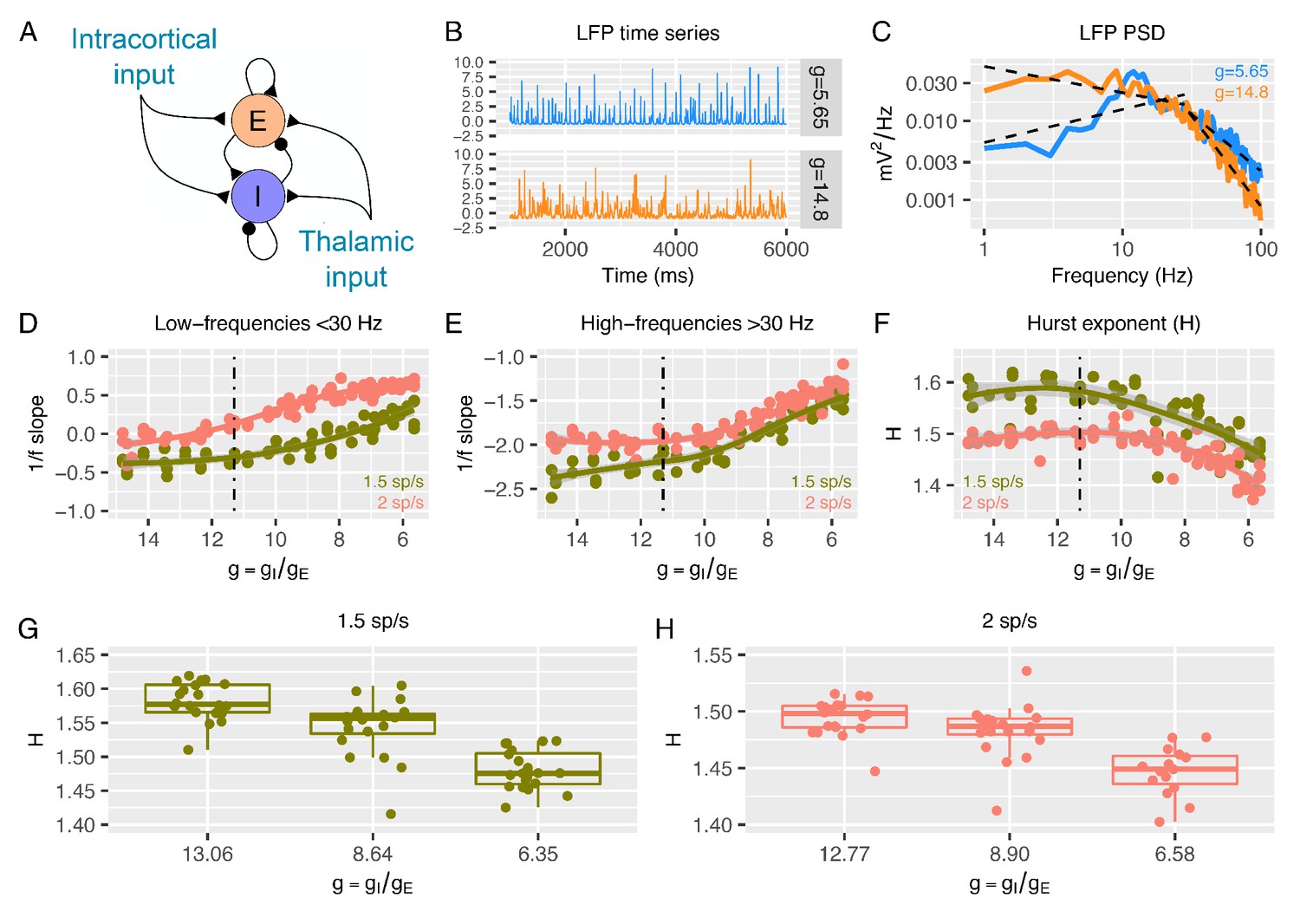
Predictions from a recurrent network model of how the low- and high-frequency slopes of the LFP power spectrum and H change with the variation in relative ratio of inhibitory and excitatory synaptic conductances.
Panel A shows a sketch of the point-neuron network that includes recurrent connections between two types of populations: excitatory cells (E) and inhibitory cells (I). Each population receives two types of external inputs: intracortical activity and thalamic stimulation. Panels B and C show examples of normalized LFP times-series and their corresponding PSDs generated for two different ratios between inhibitory and excitatory conductances (). The low- and high-frequency slopes of the piecewise regression lines that fit the log-log plot of the LFP PSDs are computed over two different frequency ranges (1-30 Hz for the low-frequency slope and 30-100 Hz for the high-frequency slope). The relationship between low-frequency slopes (panel D), high-frequency slopes (panel E) and H values (panel F) are plotted as a function of for two different firing rates of thalamic input (1.5 and 2 spikes/second). The reference value of (which has shown in previous studies to reproduce cortical data well) is represented by a dashed black line. In panel G and H, we show H values in 3 different groups of (high, medium and low ), with the same number of samples in each group.
Figure 1—figure supplement 1
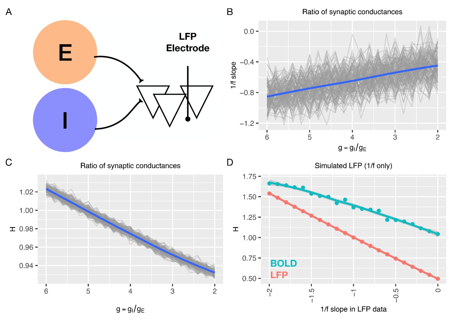
In silico predictions from a non-recurrent model of how 1/f slope and H change with E:I ratio ().
Panel A shows a schematic of the model (Gao et al., 2017) that computationally generates LFPs based on manipulated E:I ratios. For parameters utilized in this model, see Supplementary file 1. Panel B reproduces the relationship reported in Gao et al., between 1/f slope and E:I ratio. All 128 simulated channels are shown in gray, and their average is shown in blue. Panel C shows the relationship between H and E:I ratio from the Gao et al., model. Panel D shows H computed on simulated LFP where the 1/f slope is prespecified. H computed on LFP data is shown in pink. The simulated BOLD signal (simulated in the same way as data from the recurrent model) is plotted in cyan.
Figure 1—figure supplement 2
1/f slope estimation with the FOOOF algorithm.
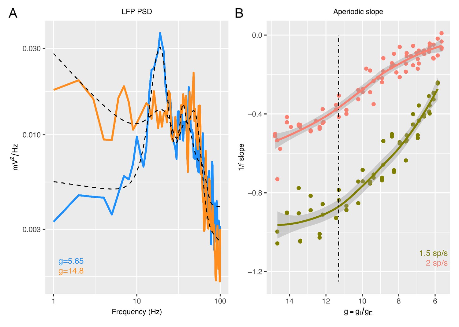
Panel A provides two examples of the LFP PSD generated from the recurrent model for different values of the E:I ratio or (blue, = 5.65; orange, = 14.8). Plotted over the PSDs are the FOOOF algorithm (Haller, 2018) model fit (dotted lines), which captures both the aperiodic signal along with the periodic oscillatory signals. Panel B shows how 1/f slope computed from FOOOF changes as a function of for two different types of thalamic input.
Figure 2 with 2 supplements
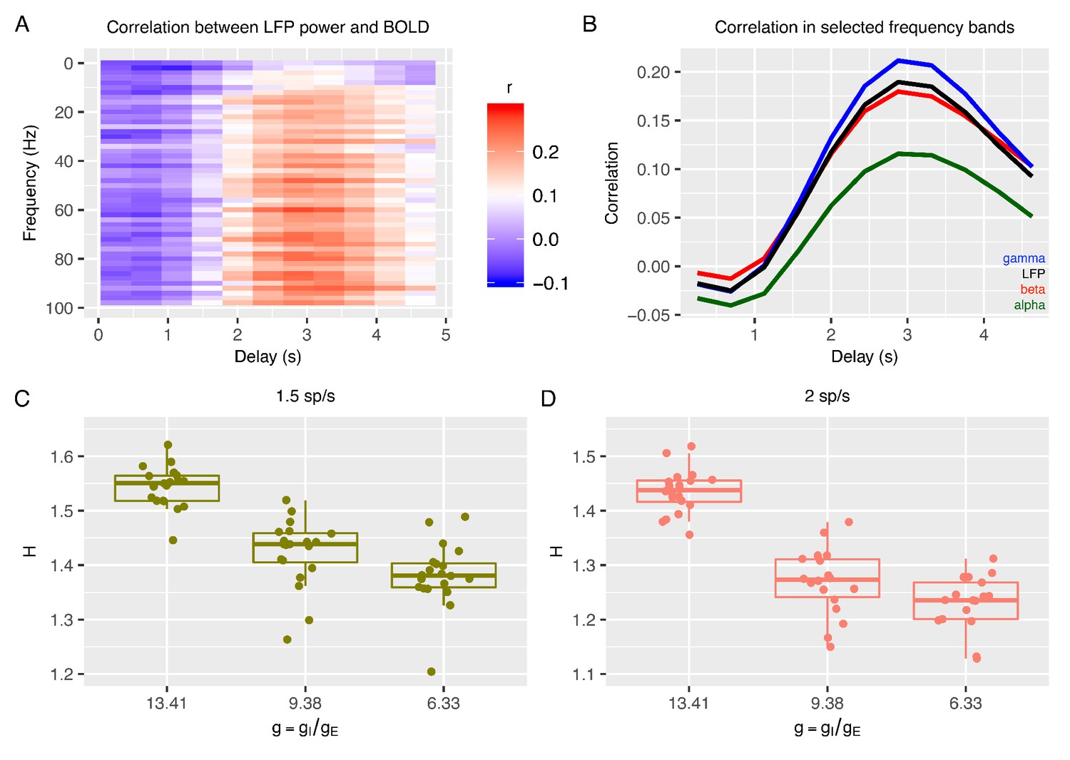
Relationship between E:I ratio from the recurrent model and H measured in simulated BOLD response.
Panel A shows time-lagged Pearson correlations between LFP power across a range of different frequencies and the BOLD signal. Panel B shows the correlation between LFP power and the BOLD signal in selected frequency bands. The following four LFP bands are considered: alpha (8–12 Hz), beta (15–30 Hz), gamma (40–100 Hz) and the total LFP power (0–100 Hz). The relationship between E:I ratio (g) and H in simulated BOLD is shown in panels C and D with two different firing rates of thalamic input (1.5 and 2 spikes/second).
Figure 2—figure supplement 1
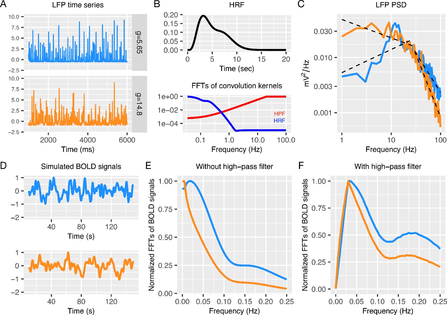
Simulating BOLD signal from LFP data generated by the recurrent model.
Panel A shows two example LFP time-series for different values of E:I ratio or (blue, = 5.65; orange, = 14.8). Panel B shows the hemodynamic response function (HRF) from Magri et al., 2012 (top) and the PSDs from Fast Fourier Transforms (FFT) (bottom) on the HRF (blue) and a high-pass filter (HPF) (red). Panel C shows LFP PSDs. BOLD signal was simulated from LFP data as the result of an inverse FFT of the product of multiplied HRF, HPF, and LFP spectra: FFT(BOLD) = FFT(LFP)FFT(HPF)[FFT(HRF) + η], where η is a constant white noise term. Panel D shows the simulated BOLD signals from this process. Panels E and F show the PSD when a high-pass filter was or was not used. In particular, BOLD spectra in Panel F show the distinctive properties such as peak frequency (≈ 0.03 Hz) and low frequency to high frequency power ratio (from 1.5 to 4) observed in previous resting-state fMRI studies (Alcauter et al., 2015; Allen et al., 2011).
Figure 2—figure supplement 2
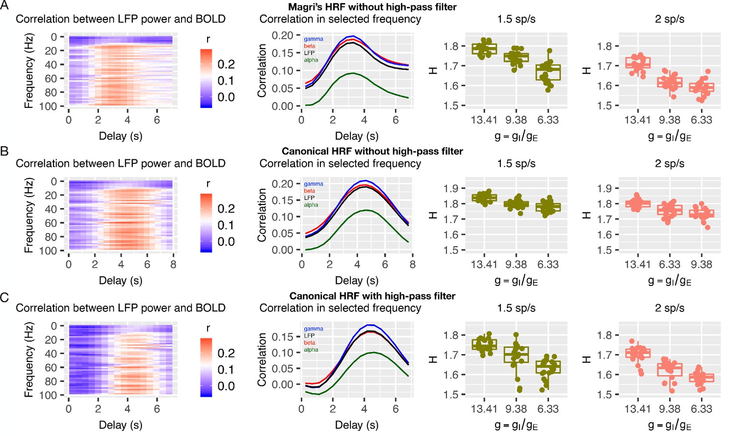
Simulated BOLD with and without high-pass filter and changes to the HRF.
Panel A shows a situation where the simulation of BOLD from LFP utilizes the HRF from Magri et al., 2012 but does not incorporate use of the high-pass filter. Panels B shows BOLD simulated from LFP with the canonical HRF without (B) and with (C) the high-pass filter. In the far left column are time-lagged correlations between LFP power over a range of frequencies as a function of the time-delay. The middle column shows LFP power correlations with BOLD in selected frequency bands. The far right column shows plots for how is related to H in BOLD for each situation.
Figure 3 with 2 supplements

Changes to H after chemogenetic DREADD manipulations to enhance excitability or silence excitatory and inhibitory neurons.
Panel A shows how H changes after the voltage threshold for spike initiation in excitatory neurons () is reduced in the recurrent model, thereby enhancing excitability as would be achieved with hM3Dq DREADD manipulation. Panel B shows how H changes after decreasing the resting potential of excitatory and inhibitory neurons (), as would be achieved with hM4Di DREADD manipulation. Panel C shows changes in H in BOLD from prefrontal cortex (PFC) after real hM3Dq DREADD manipulation in mice, while panel D shows changes in PFC BOLD H after hM4Di DREADD manipulation in mice. In panels C and D, individual gray lines indicate H for individual mice, while the colored lines indicate Baseline (pink), Transition (green), and Treatment (blue) periods of the experiment. During the Baseline period H is measured before the drug or SHAM injection is implemented. The Transition phase is the period after injection but before the period where the drug has maximal effect. The Treatment phase occurs when the drug begins to exert its maximal effect. The green star indicates a Condition*Time interaction (p<0.05) in the Transition phase, whereas the blue stars indicate a main effect of Condition within the Treatment phase (p < 0.005).
Figure 3—figure supplement 1
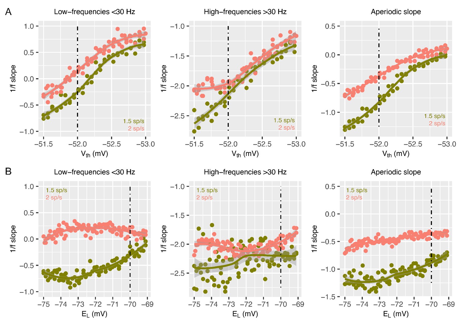
1/f slope computed with the FOOOF algorithm after manipulations to the voltage threshold for spike initiation and resting potential for excitatory and inhibitory neurons.
Panel A shows 1/f slopes computed after the voltage threshold for spike initiation () is manipulated. Panel B shows 1/f slopes computed after the resting potential for excitatory and inhibitory neurons () is manipulated. The left column shows results when computed in the low-frequency range (<30 Hz). The middle column shows results when computed in the high-frequency range (>30 Hz). The right column shows 1/f slopes as computed by the FOOOF algorithm (Haller, 2018). In each plot, salmon color indicates simulations with a thalamic input of 2 spikes/second, while the olive color indicates thalamic input of 1.5 spikes/second.
Figure 3—figure supplement 2
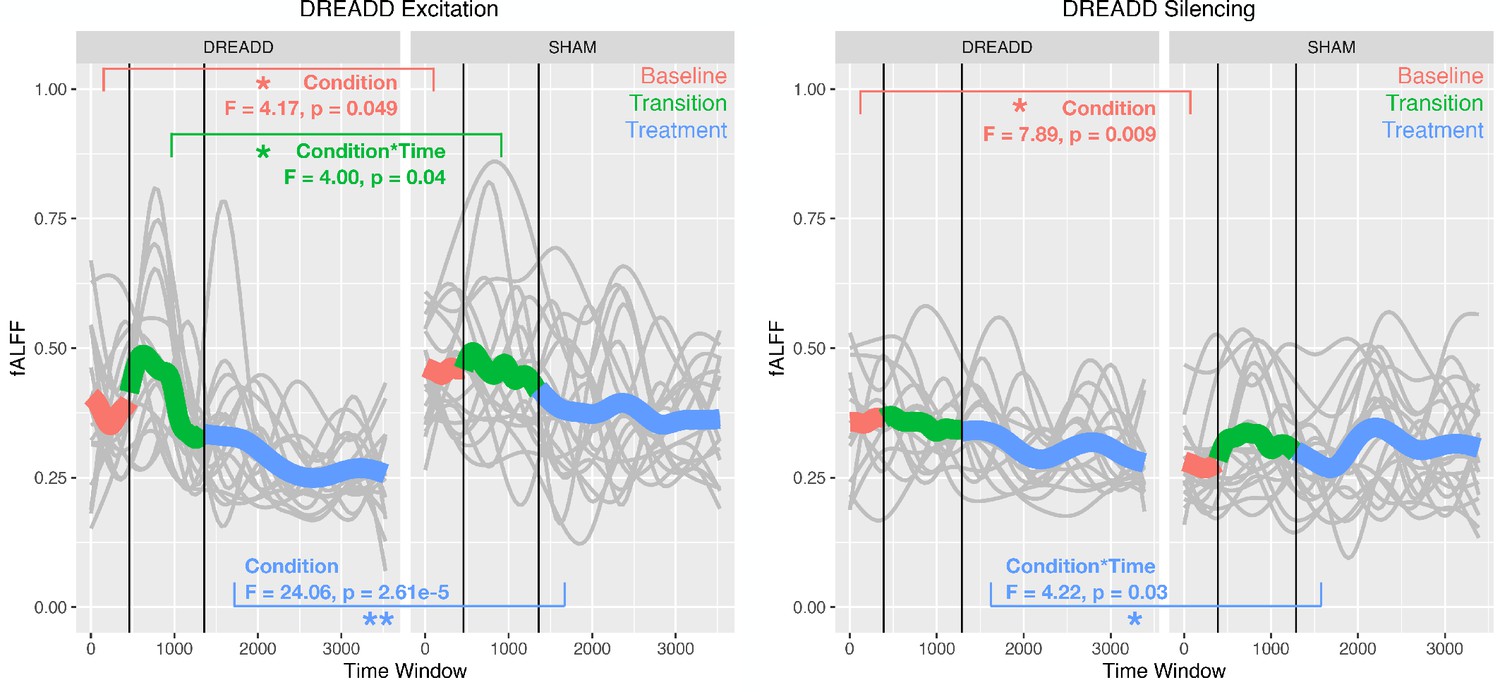
This figure shows how fractional amplitude of low frequency fluctuations (fALFF) changes in BOLD signal from prefrontal cortex (PFC) after real hM3Dq DREADD (i.e. DREADD Excitation; left panel) or after hM4Di DREADD (i.e. DREADD Silencing; right panel) in mice.
Individual gray lines indicate fALFF for individual mice, while the colored lines indicate Baseline (pink), Transition (green), and Treatment (blue) periods of the experiment. During the Baseline period fALFF is measured before the drug or SHAM injection is implemented. The Transition phase is the period after injection but before the period where the drug has maximal effect. The Treatment phase occurs when the drug begins to exert its maximal effect.
Figure 4
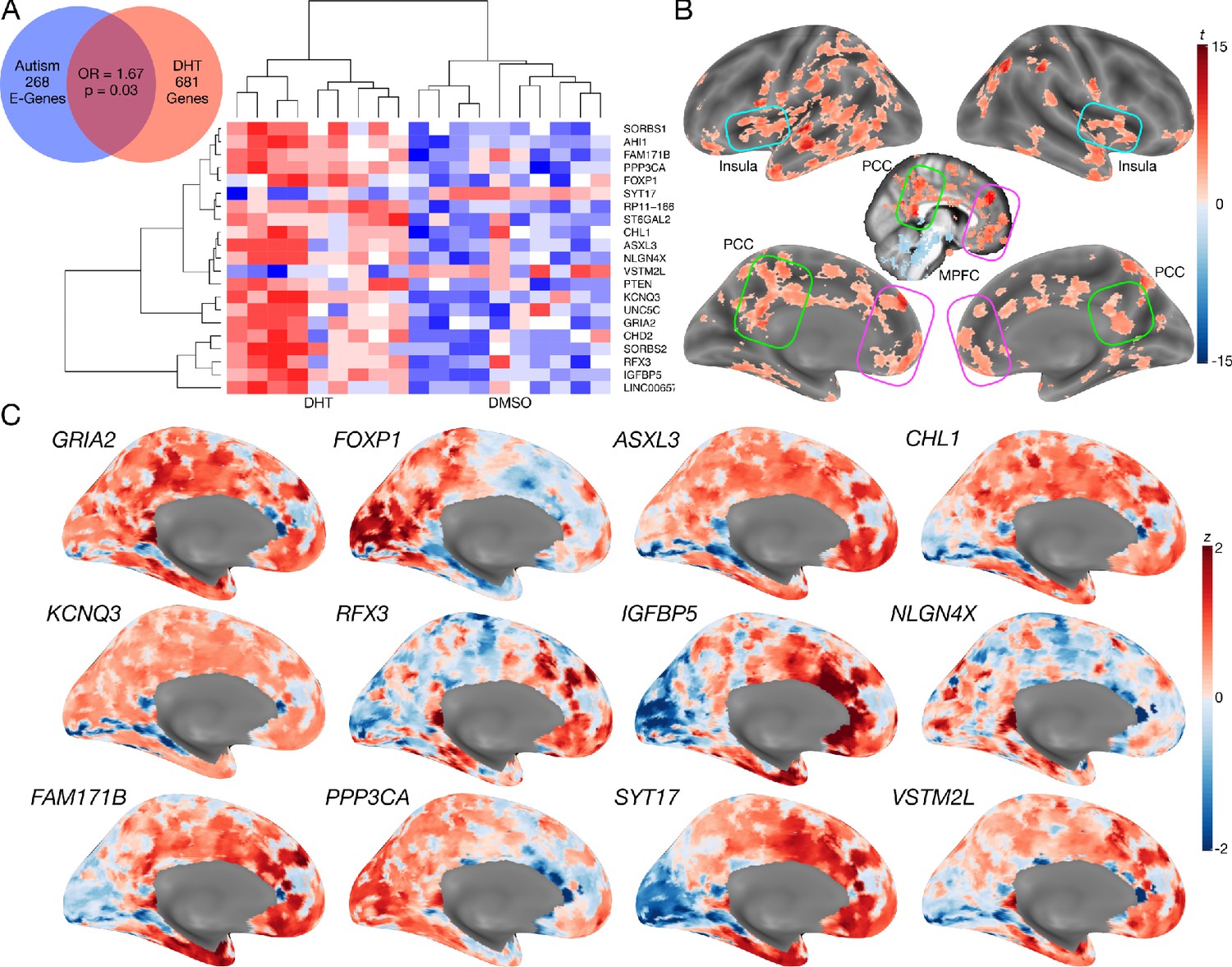
Autism-associated genes within excitatory neuronal cell types are enriched for genes differentially expressed by androgen hormones.
Panel A shows a Venn diagram depicting the enrichment between autism-associated genes affecting excitatory neurons (Autism E-Genes) and DHT-sensitive genes. Panel A also includes a heatmap of these genes whereby the color indicates z-normalized expression values. The column dendrogram clearly shows that all samples with DHT treatment are clustered separately from the control (DMSO) samples. Each row depicts the expression of a different gene. Panel B shows a t-statistic map from a whole-brain one-sample t-test on these DHT-sensitive and autism-associated genes in excitatory neurons. Results are thresholded at FDR q < 0.01. Panel C shows spatial gene expression profiles on a representative surface rendering of the medial wall of the cortex for specific genes shown in panel B. Each map shows expression as z-scores with the color scaling set to a range of −2 < z < 2.
Figure 5 with 2 supplements
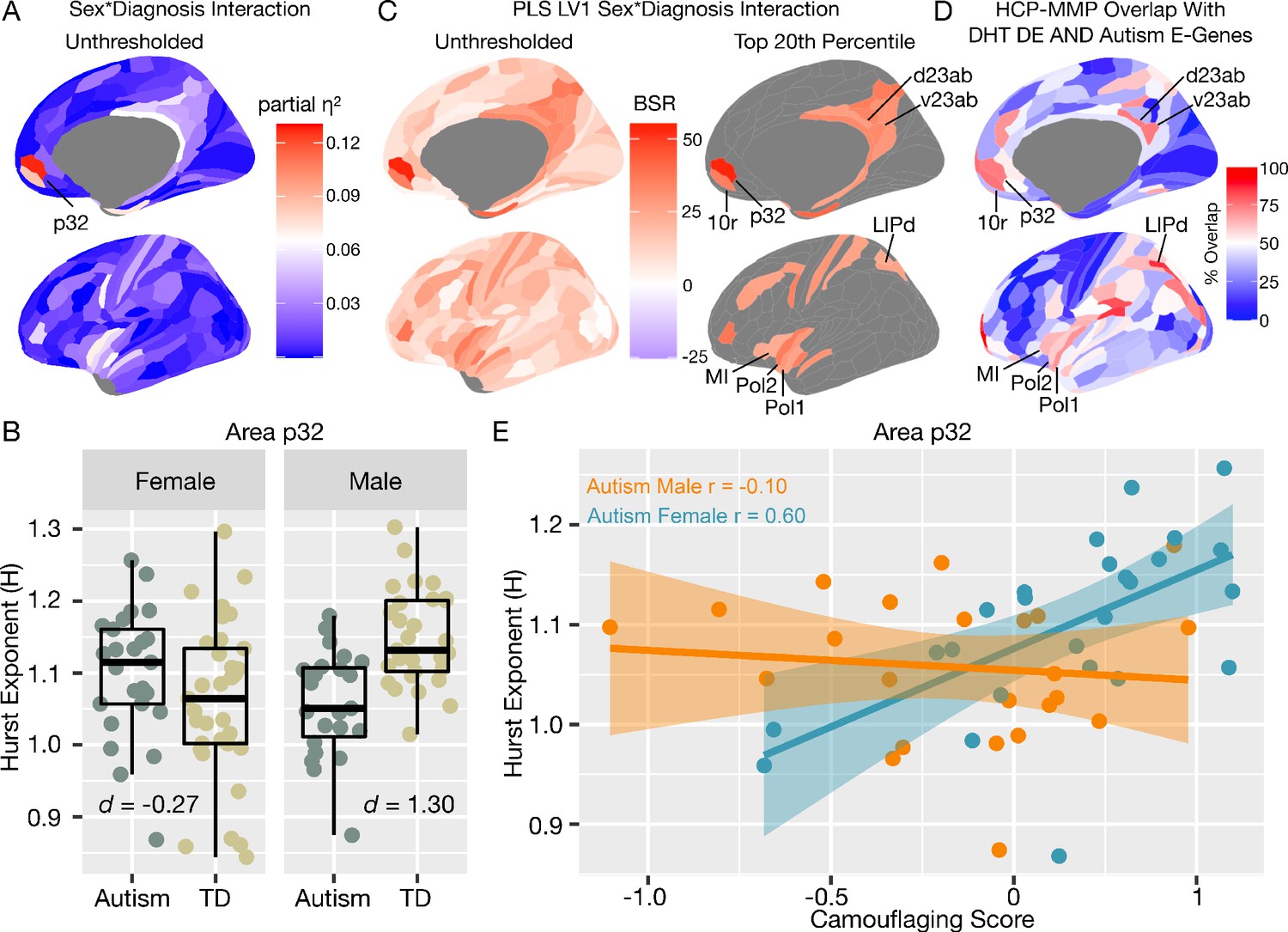
Autism rsfMRI sex-by-diagnosis interaction results.
Panel A shows unthresholded and thresholded with FDR q < 0.05 mass-univariate results for the sex-by-diagnosis interaction contrast. Panel B shows H estimates from vMPFC (area p32) across males and females with and without autism. Panel C shows partial least squares (PLS) results unthresholded and thresholded to show the top 20% of brain regions ranked by bootstrap ratio (BSR). Panel D shows the percentage of voxels within each HCP-MMP parcellation region that overlap with the DHT-sensitive AND autism-associated genes affecting excitatory neurons (Autism E-Genes) map shown in Figure 4B. Panel E shows correlation between vMPFC H and behavioral camouflaging score in autistic males (orange) and females (blue).
Figure 5—figure supplement 1
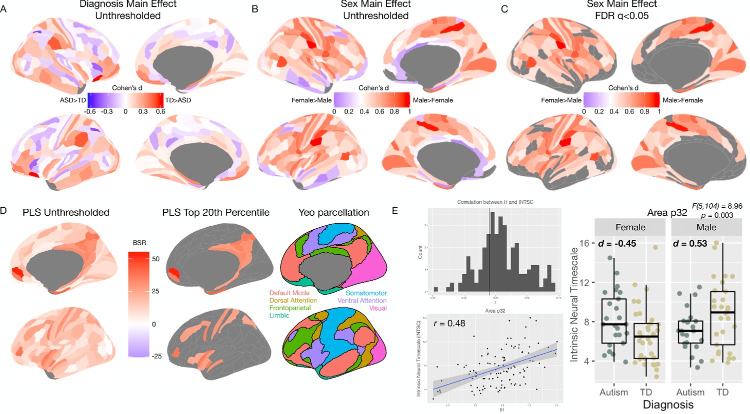
Human rsfMRI data univariate main effects, PLS overlap with resting state networks, and effects on intrinsic neural timescale.
Panel A shows the unthresholded standardized effect size map for the main effect of Diagnosis in human rsfMRI data from the MRC AIMS dataset. No regions survive at FDR q < 0.05 for this comparison. Panel B shows a similar unthresholded standardized effect size map for the main effect of Sex. Panel C shows that several regions (61% of regions) pass at FDR q < 0.05 and all are in the directionality of Male >Female. Panel D shows the PLS results next to the seven cluster rsfMRI parcellation from Yeo et al., 2011. This panel shows prominent overlap between most important PLS regions and the default mode network (DMN). Panel E shows a histogram of the correlation between H and the intrinsic neural timescale (INTSC) metric reported by Watanabe et al., 2019 across all brain regions (top left). In the bottom left of panel E is a scatterplot showing the correlation between H and INTSC for vMPFC (Area p32). The far right of panel E is a plot to descriptively show the distributions and effect sizes for the sex-by-diagnosis interaction effect in area p32 for INTSC.
Figure 5—figure supplement 2
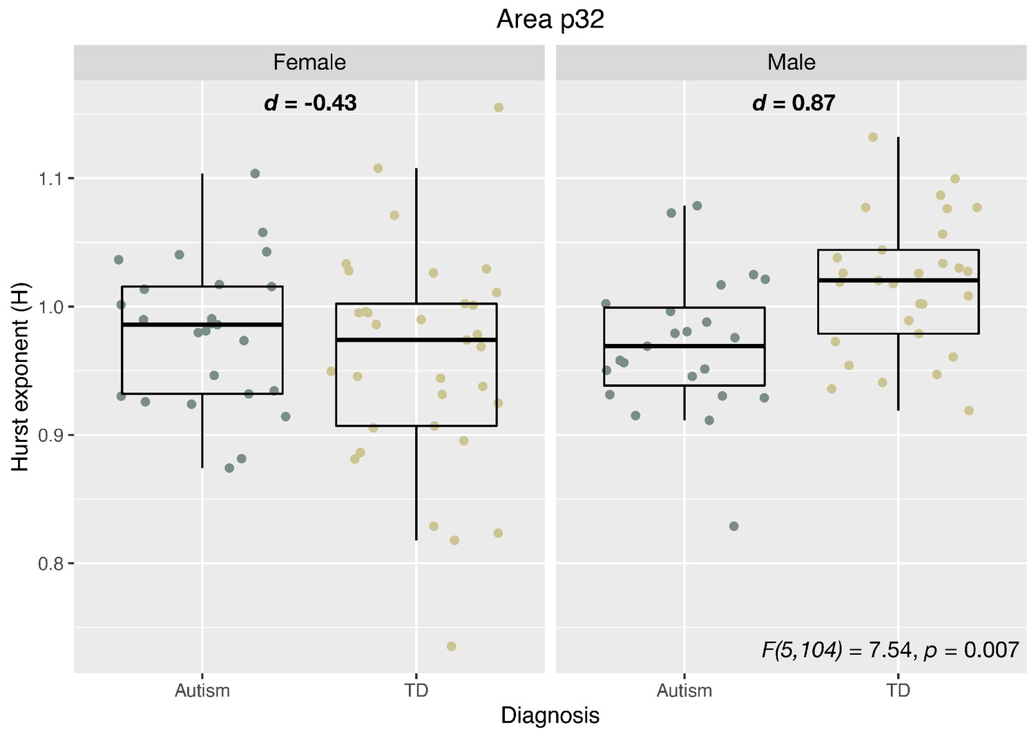
This figure shows results from region p32 when H is computed first from all voxels and then averaged for a mean H estimate across all voxels from the p32 region.
Tables
Table 1
Results from DREADD excitation manipulation.
F-statistics (p-values in parentheses) for main effects of time, condition, and time*condition interaction for each of the 3 phases of the experiment (Baseline, Transition, Treatment). *=p < 0.05, **=p < 0.001.
| Time | Condition (DREADD - SHAM) | Time x Condition | |
|---|---|---|---|
| Baseline | 0.82 (0.372) | 0.81 (0.369) | 0.36 (0.549) |
| Transition | 5.65 (0.017)* | 3.25 (0.081) | 4.94 (0.026)* |
| Treatment | 0.61 (0.433) | 12.92 (0.001)** | 0.66 (0.418) |
Table 2
Results from DREADD silencing manipulation.
F-statistics (p-values in parentheses) for main effects of time, condition, and time*condition interaction for each of the 3 phases of the experiment (Baseline, Transition, Treatment). *=p < 0.05, **=p < 0.001.
| Time | Condition (DREADD - SHAM) | Time x Condition | |
|---|---|---|---|
| Baseline | 0.02 (0.876) | 4.01 (0.054) | 1.02 (0.137) |
| Transition | 0.04 (0.838) | 0.35 (0.561) | 1.36 (0.243) |
| Treatment | 0.40 (0.533) | 0.20 (0.673) | 0.10 (0.786) |
Table 3
Descriptive and inferential statistics for group comparisons of demographic and clinical variables.
Values in the columns for each group represent the mean and standard deviation (in parentheses). Values in the columns labeled Sex, Diagnosis, and Sex*Diagnosis indicate the F-statistic and p-value (in parentheses). Abbreviations: TD, Typically Developing; VIQ, verbal IQ; PIQ, performance IQ; FIQ, full-scale IQ; ADI-R, Autism Diagnostic Interview–Revised; ADOS, Autism Diagnostic Observation Schedule; RRB, Restricted Repetitive Behaviors; AQ, Autism Spectrum Quotient; RMET, Reading the Mind in the Eyes Test, FD: frame-wise displacement.
| TD males (N = 29) | Autistic males (N = 23) | TD females (N = 33) | Autistic females (N = 25) | Sex | Diagnosis | Sex* diagnosis | |
|---|---|---|---|---|---|---|---|
| Age | 28.00 (6.42) | 27.13 (7.14) | 26.99 (5.34) | 27.35 (6.79) | 0.14 (0.70) | 0.03 (0.85) | 0.25 (0.61) |
| VIQ | 110.62 (11.53) | 114.70 (13.04) | 120.30 (10.06) | 114.08 (12.79) | 5.33 (0.02) | 0.38 (0.53) | 5.18 (0.02) |
| PIQ | 120.00 (10.21) | 114.57 (15.70) | 117.39 (9.27) | 110.88 (17.43) | 1.49 (0.22) | 5.55 (0.02) | 0.04 (0.83) |
| FIQ | 116.97 (10.69) | 116.39 (14.15) | 121.45 (8.33) | 114.16 (13.82) | 0.48 (0.48) | 3.38 (0.06) | 2.24 (0.13) |
| Camouflaging Score | - | −0.16 (0.38) | - | 0.15 (0.34) | 9.06 (0.004) | - | - |
| AQ | 15.28 (6.99) | 32.70 (8.47) | 11.97 (4.93) | 38.44 (6.34) | 0.26 (0.61) | 300.59 (2.2e-16) | 12.48 (0.0006) |
| ADI-R Reciprocal-Social-Interaction | - | 17.26 (4.77) | - | 16.56 (4.52) | 0.27 (0.60) | - | - |
| ADI-R Communication | - | 14.83 (3.50) | - | 13.40 (3.96) | 1.73 (0.19) | - | - |
| ADI-R RRB | - | 5.17 (2.35) | - | 4.24 (1.61) | 2.61 (0.11) | - | - |
| ADOS Communication | - | 3.30 (1.74) | - | 1.24 (1.30) | 21.85 (2.59e-5) | - | - |
| ADOS Social | - | 5.48 (3.45) | - | 3.48 (3.06) | 4.52 (0.03) | - | - |
| ADOS RRB | - | 1.09 (1.12) | - | 4.30 (1.61) | 61.84 (6.32e-10) | - | - |
| ADOS Communication + Social Total | - | 8.83 (4.87) | - | 4.72 (4.09) | 10.07 (0.002) | - | - |
| RMET | 27.14 (3.59) | 20.83 (6.87) | 28.91 (2.35) | 22.84 (6.40) | 3.93 (0.04) | 42.30 (2.704e-9) | 0.01 (0.89) |
| Mean FD | 0.17 (0.05) | 0.20 (0.07) | 0.18 (0.06) | 0.04 (0.17) | 0.51 (0.47) | 1.77 (0.18) | 1.10 (0.29) |
Table 4
Baseline reference parameters of the recurrent network model.
Parameters used in Cavallari et al., 2014 with conductance-based synapses.
| A: Neuron model | |||
|---|---|---|---|
| Parameter | Description | Excitatory cells | Inhibitory cells |
| Vleak (mV) | Leak membrane potential | −70 | −70 |
| Vthreshold (mV) | Spike threshold | −52 | −52 |
| Vreset (mV) | Reset potential | −59 | −59 |
| τrefractory (ms) | Absolute refractory period | 2 | 1 |
| gleak (nS) | Leak membrane conductance | 25 | 20 |
| Cm (pF) | Membrane capacitance | 500 | 200 |
| τm (ms) | Membrane time constant | 20 | 10 |
| B: Connection parameters | |||
| Parameter | Description | Excitatory cells | Inhibitory cells |
| EAMPA (mV) | AMPA reversal potential | 0 | 0 |
| EGABA (mV) | GABA reversal potential | −80 | −80 |
| τr(AMPA) (ms) | Conductance rise time (AMPA) | 0.4 | 0.2 |
| τd(AMPA) (ms) | Conductance decay time (AMPA) | 2 | 1 |
| τr(GABA) (ms) | Conductance rise time (GABA) | 0.25 | 0.25 |
| τd(GABA) (ms) | Conductance decay time (GABA) | 5 | 5 |
| τl (ms) | Synapse latency | 0 | 0 |
| gAMPA(rec.) (nS) | AMPA conductance (recurrent) | 0.178 | 0.233 |
| gAMPA(tha.) (nS) | AMPA conductance (thalamic) | 0.234 | 0.317 |
| gAMPA(cort.) (nS) | AMPA conductance (intracortical) | 0.187 | 0.254 |
| gGABA (nS) | GABA conductance | 2.01 | 2.7 |
Additional files
-
Supplementary file 1
Parameters for E:I model: Parameters utilized in the E:I model from Gao et al., 2017, for simulating LFP data.
- https://cdn.elifesciences.org/articles/55684/elife-55684-supp1-v2.docx
-
Transparent reporting form
- https://cdn.elifesciences.org/articles/55684/elife-55684-transrepform-v2.docx
Download links
A two-part list of links to download the article, or parts of the article, in various formats.
Downloads (link to download the article as PDF)
Open citations (links to open the citations from this article in various online reference manager services)
Cite this article (links to download the citations from this article in formats compatible with various reference manager tools)
Intrinsic excitation-inhibition imbalance affects medial prefrontal cortex differently in autistic men versus women
eLife 9:e55684.
https://doi.org/10.7554/eLife.55684


