Temporal integration of auxin information for the regulation of patterning
- Laboratoire Reproduction et Développement des Plantes, Univ Lyon, ENS de Lyon, UCB Lyon 1, CNRS, INRAE, Inria, France
- Department of Stem Cell Biology, Centre for Organismal Studies, Heidelberg University, Germany
Figures
Figure 1 with 3 supplements
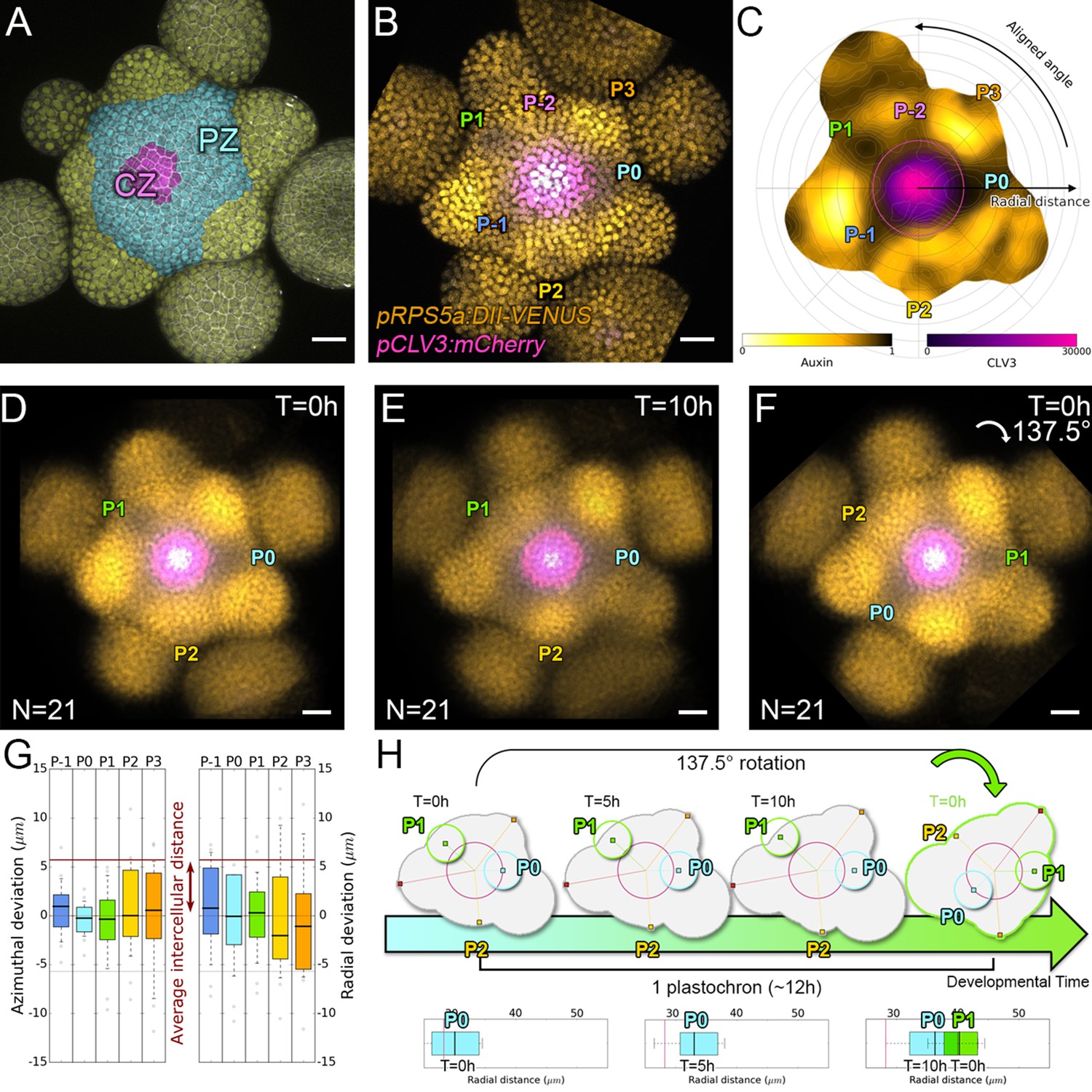
Spatial auxin distribution in the SAM follows a precise reiterative pattern.
(A) SAM radial organization. The CZ (magenta) is surrounded by the PZ (cyan). Emerging flower primordia and flowers are colored in yellow. (B). Representative expression patterns of DII-VENUS-N7 (yellow) and pCLV3:mCherry transcriptional reporter line (magenta). Primordia are indicated by color and rank. (C). Auxin map (1-qDII, yellow to black) of (B). CLV3 expression (magenta) and radial extension (circle) are shown. Black arrows depict radial distance from the center and aligned angle. (D–F). Superposition of 21 aligned SAM images at time 0 hr (D), and 10 hr (E). (F) 137.5° clockwise rotation of (D) results in a quasi-identical image of (E). See Figure 1—figure supplement 2A for non-aligned image superposition. Scale bars = 20 µm. (G). Precision in auxin maxima positioning measured using angular position deviation (azimuthal deviation, left panel) and radial direction (right panel). Red lines indicate the average cellular distance. N = 21 meristems. Colors indicate primordium ranks (P-1 blue, P0 cyan, P1 green, P2 yellow, P3 orange) (H). Space can be used as a proxy for time, as a rotation of 1 divergence angle is equivalent to a translation of 1 plastochron in time.
Figure 1—figure supplement 1
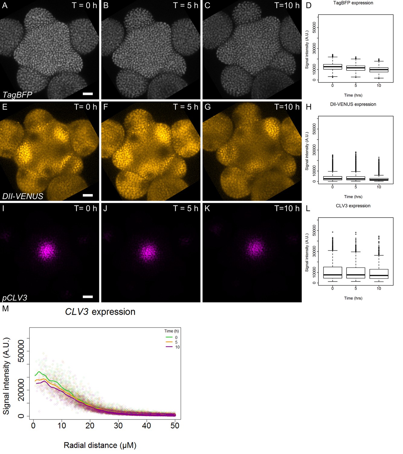
Expression pattern of qDII and CLV3.
(A–C). Time-course images of TagBFP (gray) driven by the RPS5a promoter in the qDII line. (D). Quantification of TagBFP nuclei intensity in the L1 cell layer of the meristem (N = 42991 nuclei). (E–G). Time-course images of DII-VENUS (yellow) in the qDII line. (H). Quantification of DII-VENUS nuclei intensity in the L1 cell layer. (I–K). Time-course images of pCLV3:mCherry. (I). Quantification of CLV3 nuclei intensity in the L1 cell layer (N = 6003 nuclei). Scale bars = 20 µM. (M). CLV3 quantified signal as a function of radial distance from the center at time 0, 5 and 10 hr. Each point represents a nucleus and regression curves for each time point distribution are shown.
Figure 1—figure supplement 2
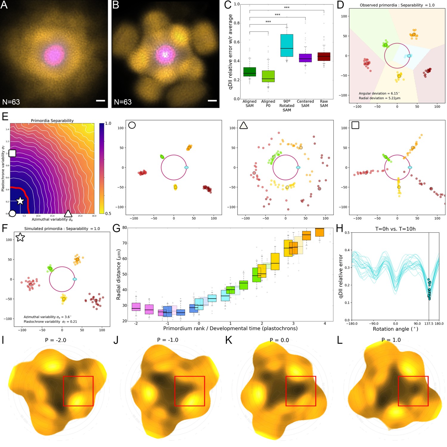
Precision in the positioning of auxin maxima enables time extrapolation.
(A). Superposition of non-registered SAM images. DII-VENUS-N7 (yellow) and TagBFP (gray) driven by the RPS5a promoter (qDII) and pCLV3:mCherry (Magenta). N = 69 meristem images. (B). Superposition of the same images as in (A) after rigid registration and rotation. Scale bars = 20 µM. (C). Distributions of relative map errors comparing an individual qDII (DII-VENUS/TagBFP) map to the average of the rest of the population. From left to right, the boxplots represent the errors obtained using the aligned image positions as in (B); the aligned image positions but only in the P0 domain; the aligned image positions compared with 90°-rotated individual maps; the raw image positions centered on the CLV3 domain; and the raw image positions as in (A). The alignment significantly reduces the error, not only in the P0 domain that is used for alignment but all over the SAM, making around three times fewer errors that the worst possible alignment. Statistically significant differences are indicated by asterisks (one-way ANOVA, p-value<0.001. (D) The positions of primordia from 21 SAMs allowed measuring the precision in angular and radial positioning. Note the perfect separability of clusters of primordia of the same rank (indicated by color). (E). A geometrical model of primordia distribution allows generating primordia positions for different values of divergence angle and plastochron variability and computing their separability. Simulations with no variability (circle) or with high variability either in divergence angle (triangle) or plastochron (square) are shown, illustrating the effect of the variability on separability of primordia. The perfect separability observed in SAM suggests that the system is restricted to a domain of low divergence angle and plastochron variability. This domain is bound by the upper values indicated by the red line. (F). Model parameters estimated from the observed angular and radial deviations of primordia (D) allow to postulate an angular variability of 3.6° and a plastochron variability of 2.5 hr for the SAM (star in (E). (G) The radial distance of an auxin maximum Pn at T = 0 hr lies between the previous maximum Pn-1 at T = 10 hr and T = 14 hr with limited variability (boxplots). 12 hr is consequently a good estimate of the plastochron, which allows positioning primordia on a developmental time axis (H). Each blue curve represents the error computed between a qDII map at T = 10 hr and the rotated map of the same SAM at T = 0 hr, applying a variable rotation angle ranging from −180° to 180°. The position on each curve corresponding to a minimal error is indicated by a blue dot. Note that all dots are robustly positioned close to 137.5° (N = 21). This evidences that performing a rotation of 137.5° (one divergence angle) is a suitable way of approximating the temporal evolution of the system after one plastochron. (I–L). Sequential auxin (1-qDII) maps showing the formation of a finger-like auxin maximum protrusion generated from the center. The red square indicates the region at the SAM at P-2 (I), P-1 (J), P0 (K) and P1 (L). See Video 1 for full sequence.
Figure 1—figure supplement 3
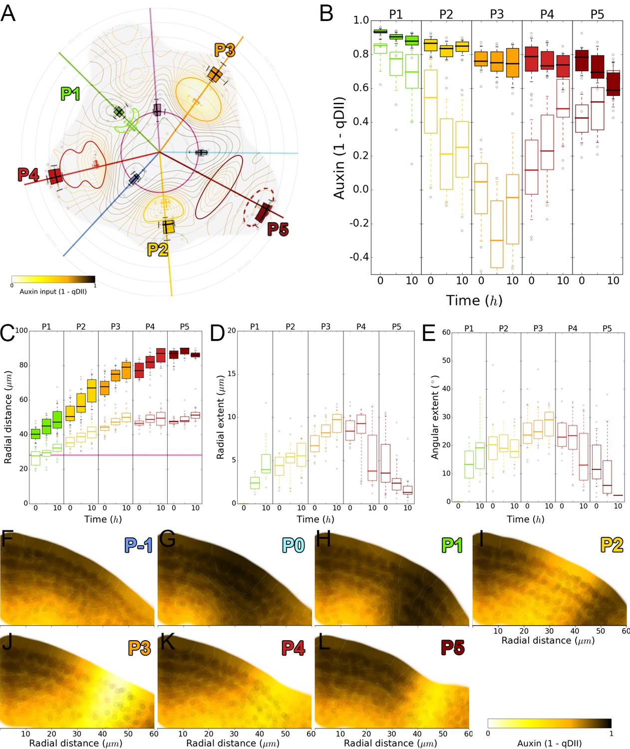
Auxin depletion dynamics.
(A). Schematic representation of auxin minimum dynamics. Auxin minima are represented as colored shapes. Minima appear from stage P1 as a crescent area (green) radially isolating the auxin maximum from the central zone, and progressively building up until its reduction to a single cell file in the organ boundary at stage P5 (dark red ellipse). Double boxplots are positioned at auxin minimum (empty) or maximum (filled) positions and show the radial and angular variability of the values. (B). Auxin values for auxin maxima (filled boxes) and minima (outline boxes) over time for each primordium. (C). Radial movement of auxin minima (outline boxes) first closely follows the one of their associated maxima (filled boxes) before stopping at a fixed distance from the center after stage P3. (D). Auxin depletion extends radially from the maxima to the center of the SAM. The depletion zone progressively widens during stages P1 to P3 before splitting in two at stage P4. (E). Auxin depletion angular extent from the auxin maximum follows a similar dynamics as in (D). (F–L). Auxin maps in longitudinal sections at the position of the primordium from P-1 (F) to P5 (L). Auxin maxima start to be formed in the L1 layer and expand towards the inner layer before moving radially. The circle shades are nuclei detected positions from which the map was generated.
Figure 2
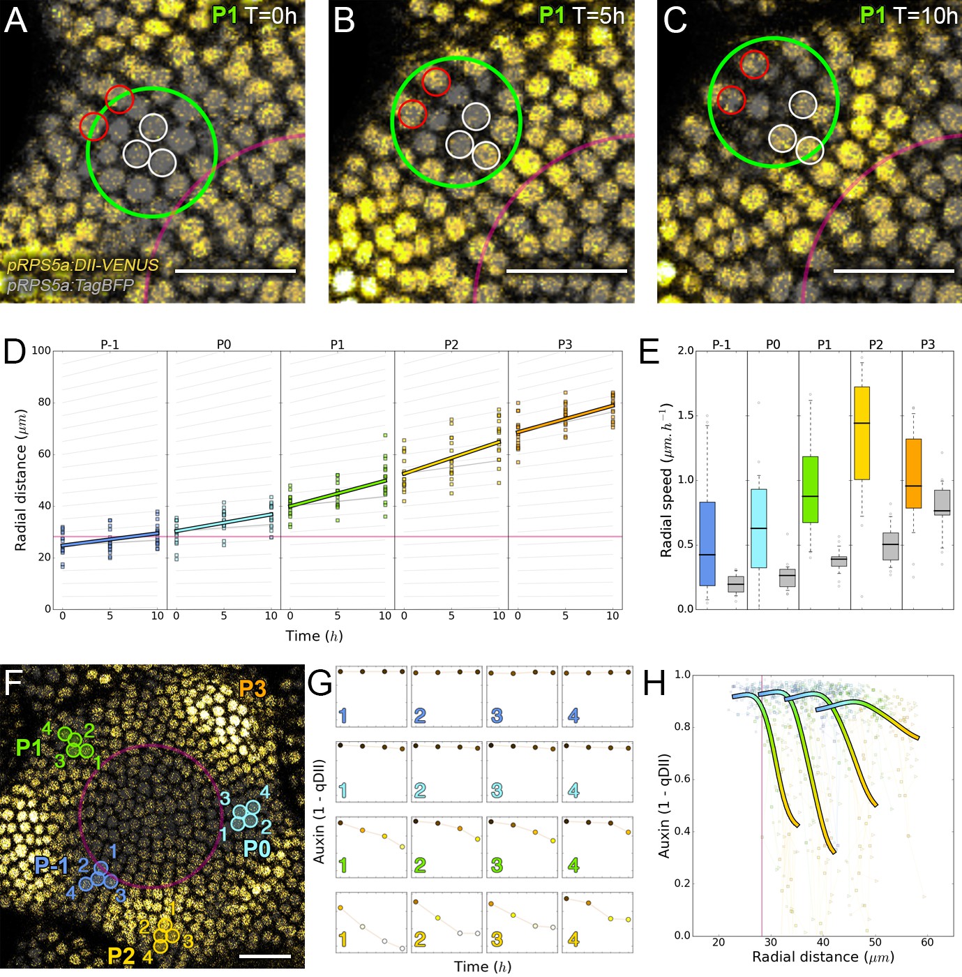
Auxin information travels as centrifugal waves in the meristem.
(A–C) Representative projection of P1 nuclei showing DII-VENUS-N7 (yellow) and TagBFP nuclei (grey) intensity changes in time. Time tracked nuclei are marked by white and red circles showing rapid decrease or increase of auxin over 10 hr, respectively. The green circle is centered on the position of the auxin maxima at each time point. The magenta line indicates the limit of the CLV3 domain. Scale bars = 20 µm. (D) Average motion of maxima (colored lines) is faster than average cell motion (grey lines). The magenta line indicates the CLV3 domain border. N = 21 meristems. (E) Compared distributions of radial motion speeds of auxin maxima (color boxplots) estimated as the slope of a linear regression per individual. Individual nucleus radial speed (gray boxplots) at the location of the maxima. N = 21 meristems. (F–G) Individual cells experience different auxin histories. Tracked cells at different locations (F; colored circles) and corresponding auxin levels (ordinate) over time (0, 5, 10, 14 hr). Scale bar = 20 µm. (H) Cellular mean auxin trajectories as a function of radial distance. Each line represents an extrapolated cell-size sector moving accordingly to cellular radial motion by its Gaussian average trajectory in radial distance (abscissa) and auxin value (ordinate). The color indicates the developmental stages at a given radial distance (P-1 = blue, P0 = cyan, P1 = green, P2 = yellow).
Figure 3 with 3 supplements
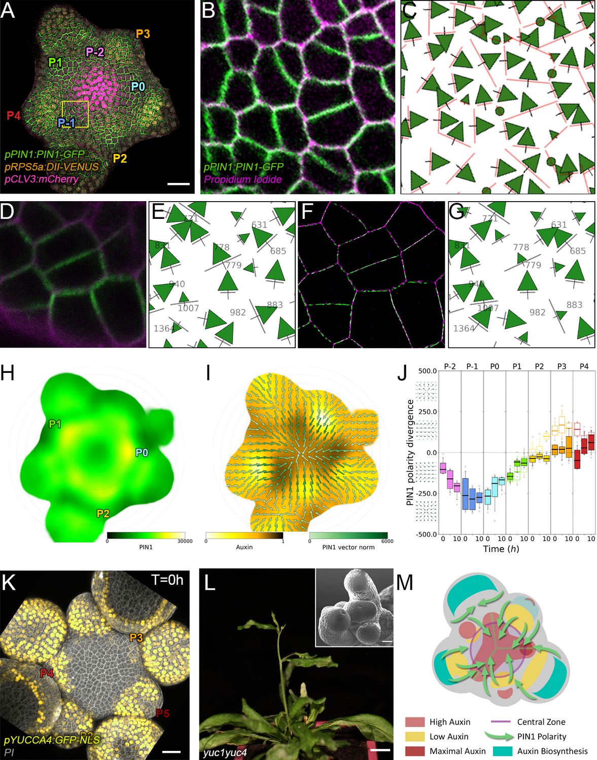
Spatio-temporal organization of auxin fluxes and biosynthesis.
(A) Co-visualization of PIN1-GFP (green), DII-VENUS-N7 (yellow) and pCLV3:mCherry (magenta). Scale bar = 20 µm. Square shows P-1 sector. (B) Magnified P-1 region of (A) PIN1-GFP (green) and PI (magenta). (C) Computed PIN1 cell interface polarities of (B). Green arrows indicate polarities with a p-value<0.1, small arrows < 0.25 and dots > 0.25. (D–G). Image of PIN1-GFP (green) and cell wall (magenta) obtained using confocal (D) or super resolution (SRRF) microscopy (F) and respective PIN1 cell interface polarities (E,G). (H) Quantification of PIN1-GFP expression. N = 4 meristems. (I) PIN1 vector map (green arrows) organization correlated with auxin distribution (yellow to black). N = 4 meristems. (J) PIN1 polarity divergence index at auxin maxima (color filled boxplots) or auxin minima (white filled boxplots) positions during organ initiation. N = 4 meristems. (K) The YUC4 auxin biosynthesis limiting enzyme is specifically expressed in developing flowers. YUC4:GFP transcriptional reporter in yellow, cell wall (PI) staining in grey. Scale bars = 20 µm. (L) yuc1yuc4 mutant inflorescence and meristem morphological defects (inset). Scale bars are 10 mm and 20 µm (inset). (M) Schematic representation of the tissue-scale organization of auxin transport and biosynthesis in relation to auxin distribution.
Figure 3—figure supplement 1
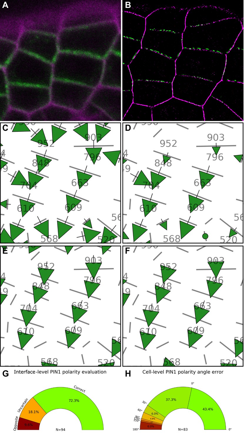
Validation of PIN1 polarity vectors with super resolution microscopy.
(A) Confocal projection of PIN1-GFP (green) and cell wall (magenta) signals. (B) SRRF (Super Resolution Radial Fluctuation) image of the cells shown in (A). PIN1-GFP (green) and cell wall (magenta). (C) PIN1 cell interface polarity orientations of (A). Green arrows indicate polarities with a p-value<0.1, small arrows < 0.25 and dots > 0.25. (D) Extracted PIN1 interface polarities from SRRF image. (See Supplementary Methods three for details). Resulting cell polarities from confocal (E) and SRRF (F) images. (G) Quantification of PIN1 cell interface polarity orientation differences between confocal automated detection and manually extracted SRRF. The donut plot shows that the majority of PIN1 interface polarities (N = 94 interfaces) are correct. Uncertain polarities due to lack of consensus between expertized and automatic detection or opposite polarity are shown. (H) Comparison of extracted PIN1 cell polarities between SRRF and confocal images. The percentage of cells with a deviation angle from 0° to 180° is indicated. 80.7% of cell polarities have a deviation below 30°. See Supplementary Methods three for detailed description of the quantification.
Figure 3—figure supplement 2
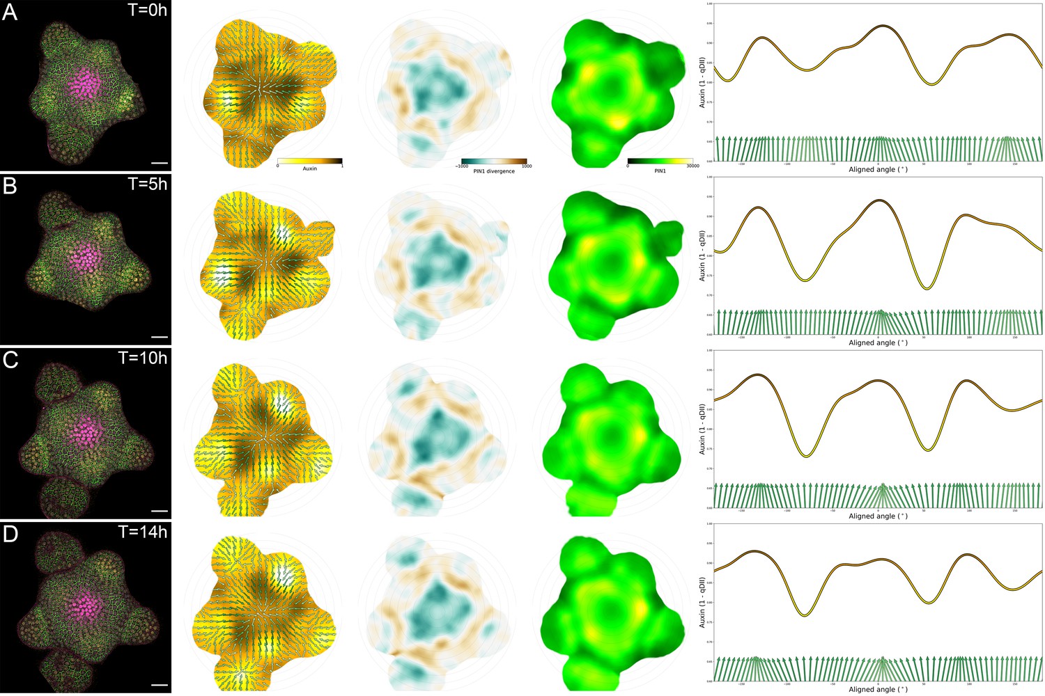
Tissue-scale PIN polarity distribution.
(A–D) From left to right, first column: Representative confocal projection of the L1 cell layer of DII-VENUS (yellow), PIN1-GFP (green) and CLV3 (magenta) during a 14 hr time-course: T = 0 (A), T = 5 (B), T = 10 (C) and T = 14 (D). Second column: Average PIN1 vector maps (green arrows; N = 4 SAMs) and auxin maps (yellow to black). Third column: local PIN1 convergence map. Blue represents convergence while brown represents divergent vectors. Forth column: map of PIN1 expression levels (green to yellow). Fifth column: circumferential distribution of auxin values (yellow to dark line) at a 35 µM radial distance and the corresponding PIN1 vector fields (green arrows). Vectors perpendicular to the axis are pointing towards the center of the SAM.
Figure 3—figure supplement 3
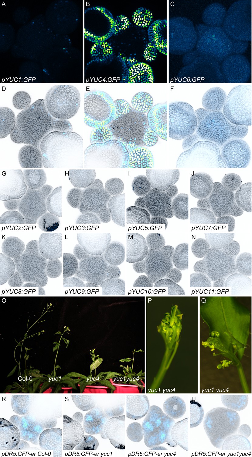
Expression patterns of YUC genes and phenotypes of yuc mutants.
(A–N) Expression patterns of YUC genes in the SAM. Expression was analyzed using transcriptional GFP reporter lines for the 11 YUC genes (GFP: Blue to green) in SAM stained with propidium iodide (PI; gray). (A–C) show the expression of GFP alone for the three YUC with expression in the SAM. All images were acquired with identical settings but in (C) the GFP signal was enhanced to ease visualization. (O–Q) Representative images of adult Col-0, yuc1, yuc4, and yuc1yuc4 mutant plants. (P–Q) Inflorescences of yuc1yuc4 mutant showing defects in flower positioning and development. (R–U) Meristem enlargement and altered auxin transcriptional responses (visualized using pDR5:GFP) in yuc1, yuc4 and yuc1yuc4 mutants. DR5 expression (Blue to green); cell wall staining with PI (gray).
Figure 4 with 1 supplement
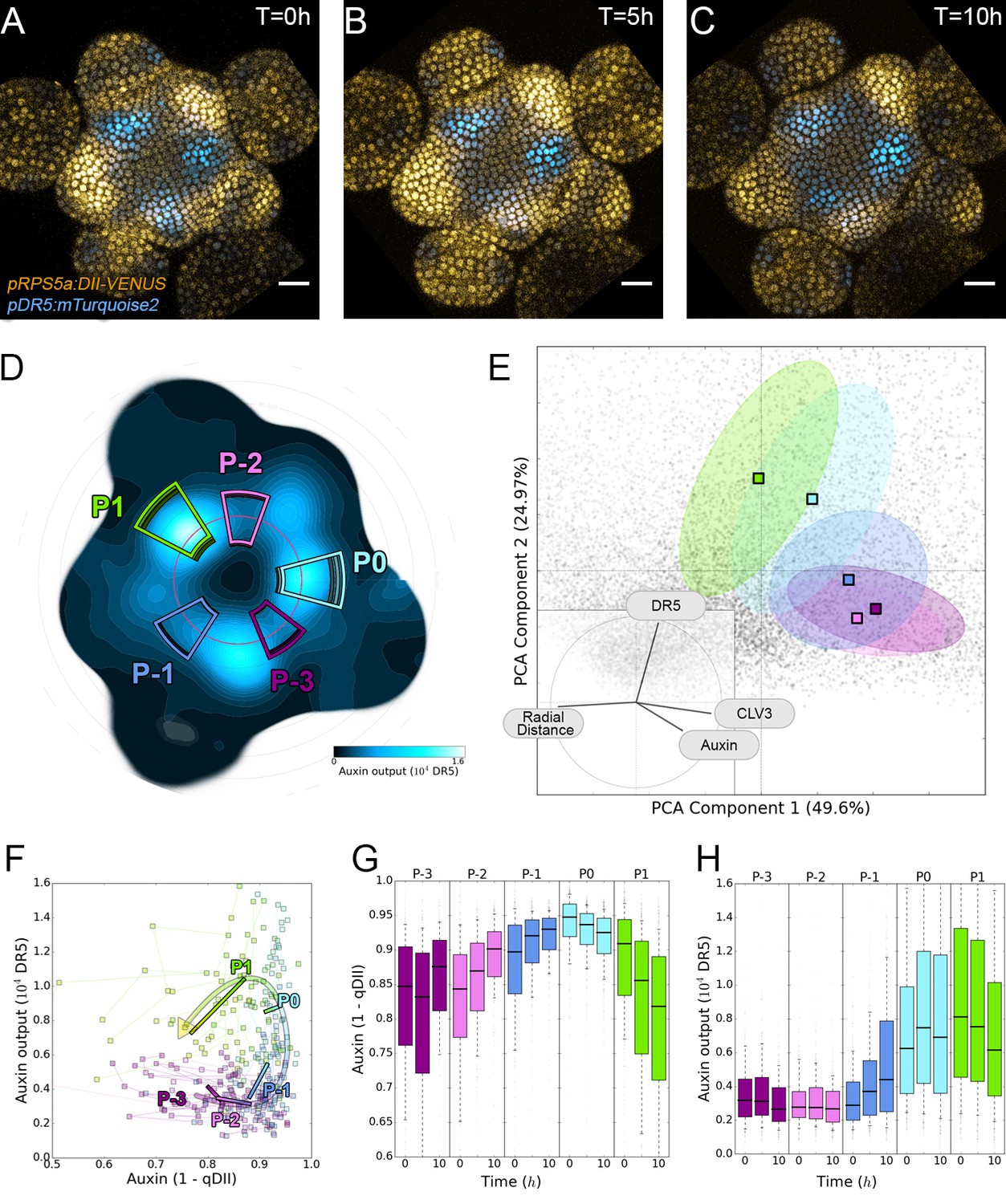
Auxin and its transcriptional output show a complex non-linear relationship.
(A–C). Time-lapse images of representative projections of DII-VENUS-N7 (yellow), TagBFP nuclei (grey) and pDR5:mTurquoise2 (cyan). Scale bars = 20 µm. (D). Quantified DR5 expression map (black to cyan). Colored sectors show the tissue areas where primordia are located (P-3 to P1). N = 21 meristems. (E). Principal Component Analysis (PCA) showing absence of correlation (orthogonality) between auxin and DR5 at the tissue scale. Colored ellipses show the consistent pattern associated with each primordium stage (from P-2 to P1 using the same colors as in (D)). (F). Auxin and DR5 non-linear relationship in primordia. Cells from P-3 to P1 are indicated with the color code used in (D). Lines represent the regression of auxin and DR5 medians in time. (G–H). Auxin (G) and DR5 (H) expression in primordia. Boxplots use the same color code for primordia as in (D). N = 21 meristems.
Figure 4—figure supplement 1
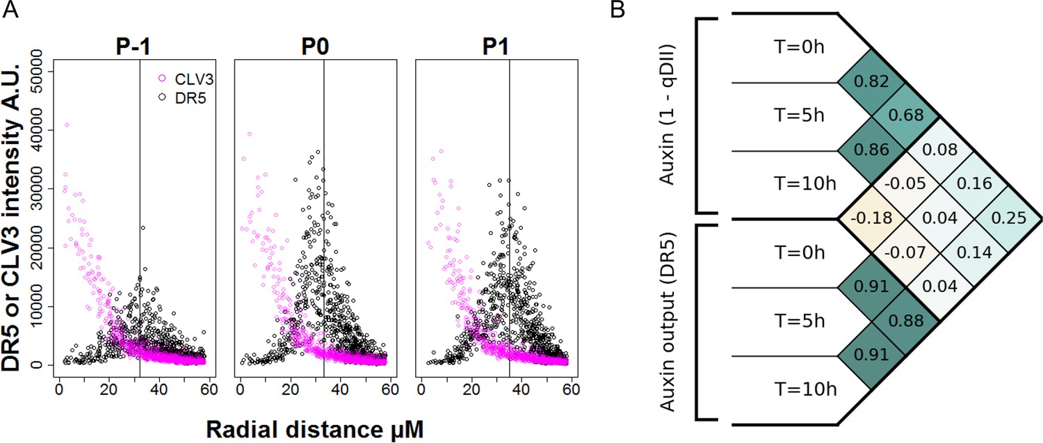
Precision in DR5 radial positioning and Pearson correlation analysis of DR5 expression and auxin levels.
(A). Radial distribution of pCLV3:mCherry (magenta circles) and pDR5:mTurquoise2 expression (black circles) at different locations of the SAM (P-1 to P1). N = 21 SAM. Each point represents a nucleus. The vertical line indicates the mean for DR5 radial distribution. (B). Pearson correlation coefficients computed on tracked cellular values of auxin levels (1-qDII) and of transcriptional output (DR5) in the entire PZ. The considered variables are the levels at time T = 0 hr, T = 5 hr and T = 10 hr, the sum of auxin input from T = 0 hr to T = 5 hr and from T = 0 hr to T = 10 hr, and the variations in DR5 levels from T = 0 hr to T = 5 hr and from T = 0 hr to T = 10 hr. No significant positive correlations are found between input and output variables.
Figure 5 with 2 supplements
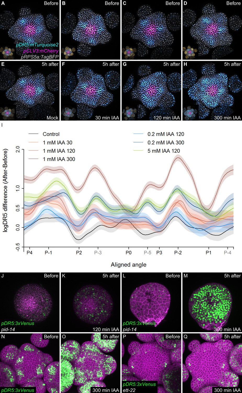
Temporal integration of auxin concentration regulates transcription.
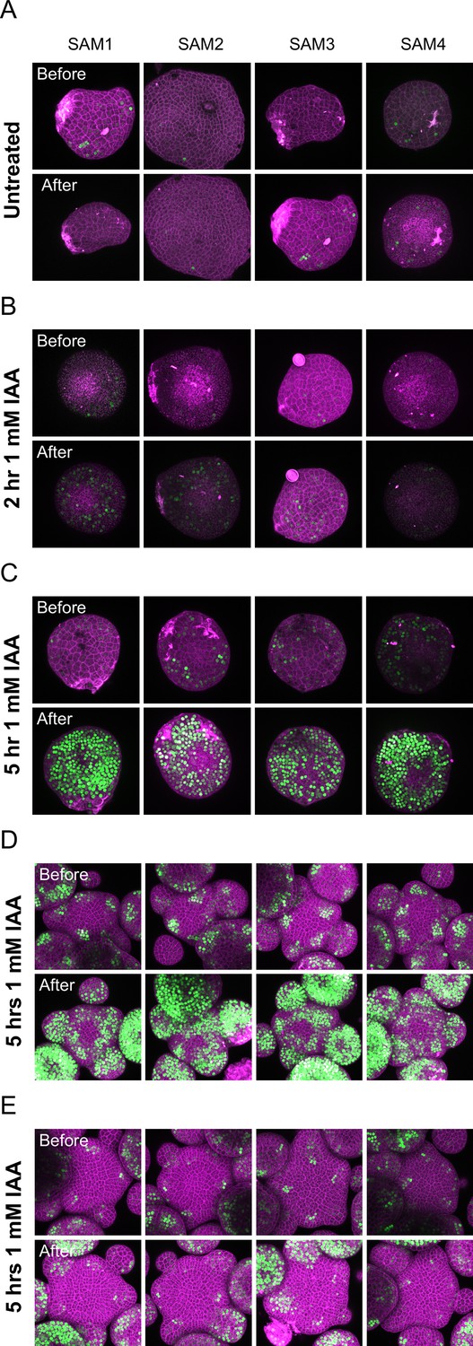
(A–I) Activation of the DR5 reporter with different concentrations of auxin and durations of treatments. pDR5:mTurquoise2 expression before auxin treatment (A–D) and 5 hr after the end of the auxin treatment: mock (E) or 1 mM IAA treatment for 30’ (F), 120’ (G) or 300’ (H). pDR5:mTurquoise (cyan), TagBFP driven by pRPS5a (gray) and pCLV3:mCherry (magenta) labelled nuclei are shown. Inset: DII-VENUS-N7 (yellow) from the same meristem. Quantification of DR5 expression in the PZ after auxin treatments. (I). Average DR5 response in the PZ with different auxin concentrations and treatment durations. Confidence intervals (shade) and regression (line) shows log(DR5) expression along the circumference of the PZ (aligned angle) of control (gray) or IAA (color) treated meristems. For simplicity only the angular position of primordia are indicated (in grey, presumptive positions). (J–M). Transcriptional response to auxin treatment of different durations in pid-14. pid-14 pDR5:3xVENUS SAM treated with IAA for 120’ (J,K) or 300’ (L,M) are shown. (N–Q). Transcriptional response to a 300’ auxin treatment in ett mutants. Control Col-0 pDR5:3xVENUS-N7 (N,O) and ett-22/arf3 pDR5:3xVENUS-N7 (P,Q) meristems treated with auxin for 300’.
Figure 5—figure supplement 1

Time integration in the control of transcription in response to auxin.
(A–H) Degradation of DII-VENUS-N7 after different periods of 1 mM auxin treatment. DII-VENUS-N7 distribution before auxin treatment (A–D) and right after the end of the auxin treatment: mock (E) or 30’ (F), 120’ (G) or 300’ (H) DII-VENUS-N7 (yellow) and pCLV3:mCherry (magenta) labelled nuclei are shown. (I) Quantification of auxin (1-qDII) in the PZ after the treatments shown in Figure 5H–I. Each profile shows auxin levels right after the end of each treatment. Each dot represents a nucleus (Mock N = 1638, 30’ 1 mM auxin N = 2026, 120’ 1 mM auxin N = 875, 300’ 1 mM auxin N = 2375, 120’ 0.2 mM auxin N = 1536, 300’ 0.2 mM auxin N = 1981 and 120’ 5 mM auxin N = 2302). The angular locations of primordia are indicated. (J–L). The effect of in planta auxin treatment of different durations (one treatment a day for five consecutive days) on organ positioning in Col-0. Flowers positioned at 90° (J) or co-inserted on a node (K) can be observed (here after a 120’ 1 mM auxin treatment). (L) Percentage of plants with phyllotaxis defects in the different treatments (0, 0.2, 1 and 5 mM auxin for 30’, 120’ or 300’ once a day during five consecutive days. (M–P) Representative images of inflorescences and meristems of Col-0 (M and O) and ett-22/arf3 mutant (N and P) showing phyllotactic defects such as co-initiations (N) and opposite organ positioning (P). (Q–S) Representative image of a pDR5:mTurquoise2 (Cyan) pCLV3:mCherry (pink) meristem treated with mock or the histone deacetylase inhibitor TSA. Red arrow in (R) indicates P-1 where activation of DR5 can be observed. (S). Quantification of DR5 expression in the PZ epidermal cell layer of (Q) and (R). Confidence intervals (shade) and regression (line) shows circumferential DR5 expression pattern in the PZ (the position of primordia from P-2 are indicated) of control (magenta) or TSA (green) treated meristems. The red arrow points to the significant activation of DR5 at P-1. DMSO N = 20 SAMs, TSA N = 20 SAMs.
Figure 5—figure supplement 2
The effect of auxin treatments of different durations on auxin transcriptional responses in pid-14 and ett-22/arf3.
(A–C) 4 examples of pid-14 pDR5:3xVENUS-N7 meristems before and 5 hr after the end of auxin treatment. Mock treated (A), 120’1 mM (B) or 300’ 1 mM auxin treatment (C). (D–E) 4 examples of meristems of Col-0 pDR5: 3xVENUS-N7 (D) or ett-22 DR5: 3xVENUS-N7 (E) treated with 1 mM IAA for 300’.
Figure 6
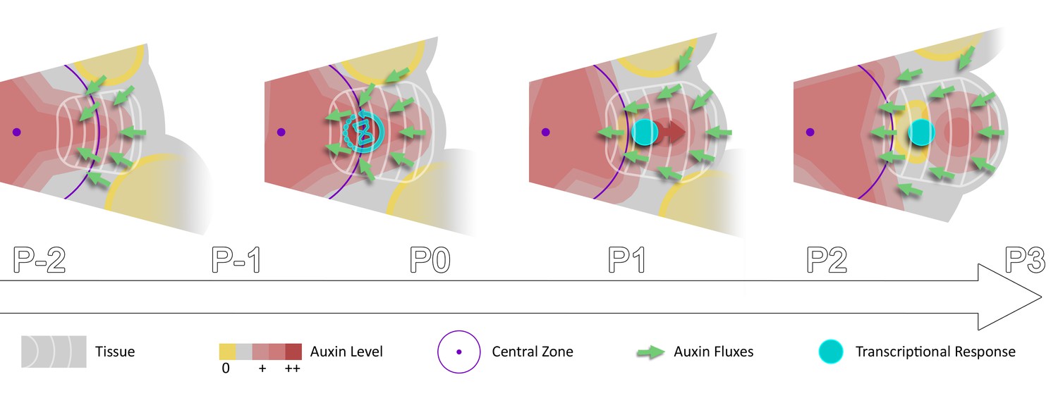
Spatio-temporal gradients of auxin translate into rhythmic organ patterning through time integration.
A maximum of auxin protrudes from a high auxin concentration zone at the CZ faster than the cell radial movement. Cells exiting the CZ that are exposed to high auxin levels progressively acquire competence for transcriptional response. This leads to activation of transcriptional responses with a delay close to the system period, the plastochron.
Appendix 2—figure 1
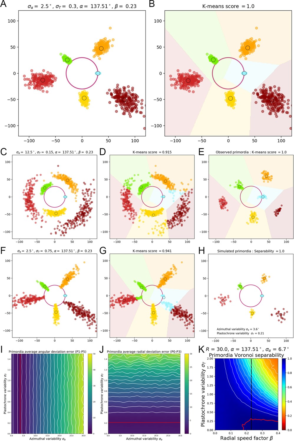
A geometrical model of primordia distribution enables estimating the plastochron variability of the SAM.
(A) Primordium points are generated from a computational phyllotactic model with a control over the variability in angular positioning and plastochron duration. (B) Linearly separable clusters in the resulting point cloud are identified using an unsupervised algorithm with prior information. The obtained labeling in primordia ranks is compared with the theoretical one to compute a separability measure. (C–D) Increasing the azimuthal variability creates clusters that are more difficult to separate and generates confusion between and . (E) The primordia points from the observed experimental data form perfectly separable clusters (F–G) Increasing the plastochron variability creates clusters that are more difficult to separate and generates confusion between and . (H–J) Measured anglular and radial deviations of both observed and simulated primordia allow to determine plausible values for the angular varibility (I) and plastochron variability (J). The prmordia sdistriibution generated with this parameters (H) is the one that metches best the observed deviation of primordia clusters. (K) Separability evaluated by varying speed coefficient and plastochron variability. Modifying the radial speed of primordia changes the tolerance of the system to azimuthal and plastochron variability. High rhythmic precision is always required to achieve seamless superposition. Red contour indicates 100% separability, white contours every lower 5%. Black line indicates experimental value of speed coefficient.
Appendix 3—figure 1
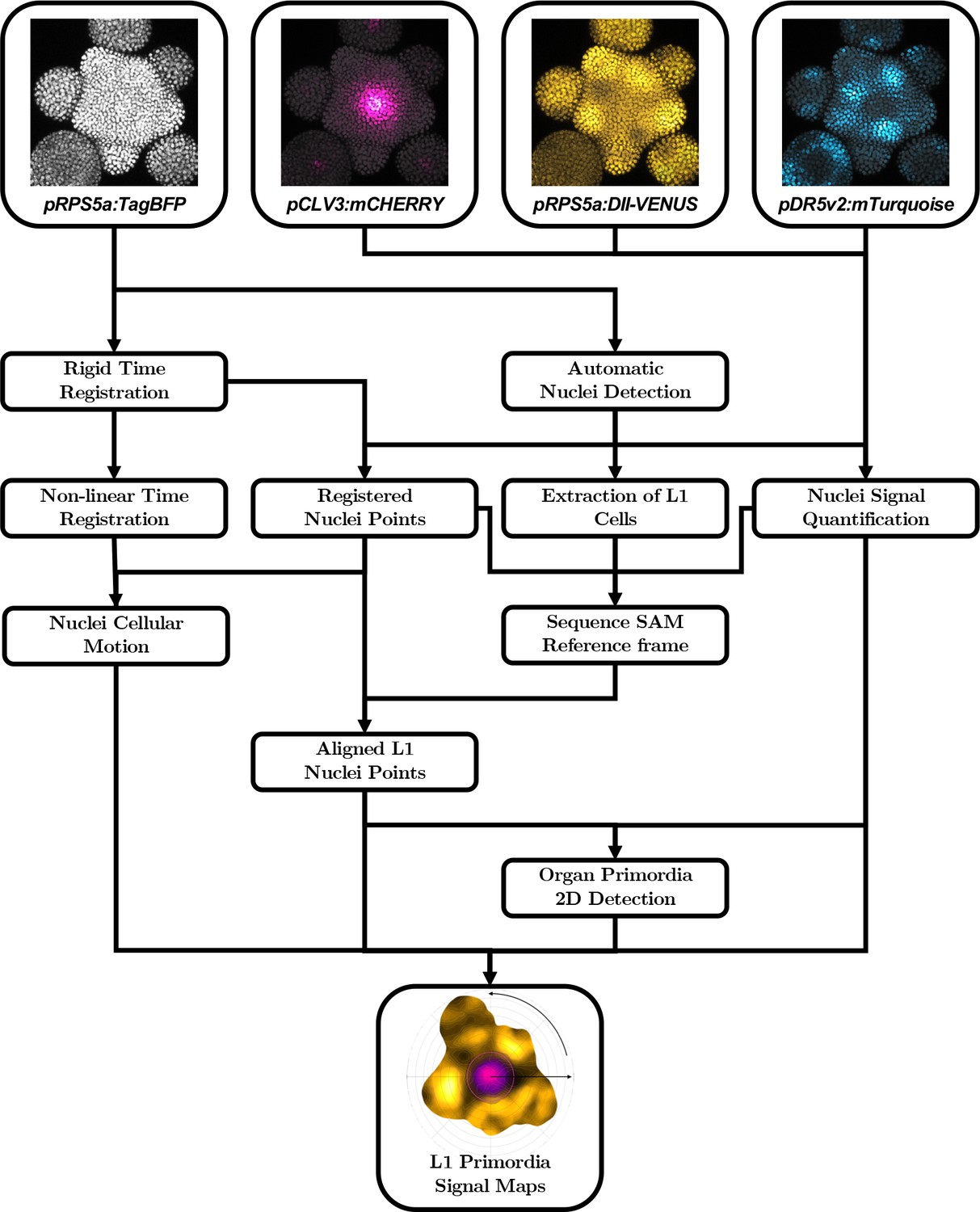
Automatic quantification pipeline for the time-lapse microscopy images of nuclei-targeted fluorescence signals.
To obtain quantitative data from the images produced under the microscope, various sequential processing steps need to be performed, from the extraction of the relevant objects (nuclei positions with their different channel intensity values) to the geometrical characterization and the spatio-temporal registration of the tissues, to finally get a complete, aligned and consistent dataset gathering all the imaged meristems.
Appendix 3—figure 2
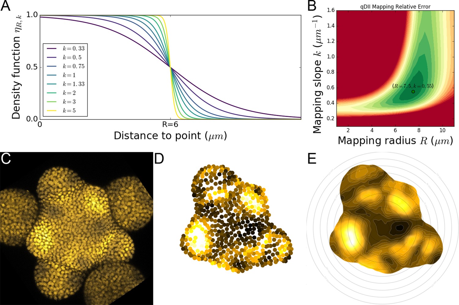
2D continuous maps of epidermal signals.
(A) To build a continuous 2D map, we diffuse the signal in space by computing a local average of discrete signal values using a kernel function whose extent and sharpness are set by two parameters and . (B). Optimal values of these parameters were determined on the signal of main interest qDII and are the ones used throughout the analyses. (C–E). Using the L1 nuclei detected in the confocal image (C) and their quantified signal values projected in 2D (D) we compute a 2D map of epidermal signal (E) in this case qDII.
Appendix 3—figure 3
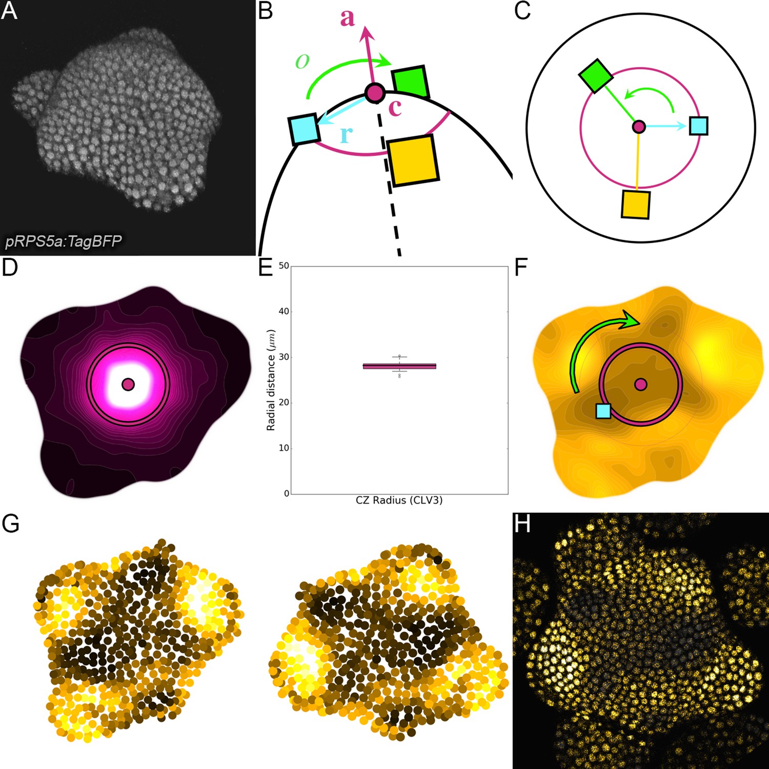
Landmark-based alignment of SAMs using 2D continuous maps.
(A) Seen in 3D, the SAM shows a dome-like structure surrounded by a spiral of primordia. (B). The center and the main axis of the dome, the direction of the last intiated primordium and the orientation of the phyllotactic spiral are key landmarks of the SAM geometry. (C). Knowing their position allows to define a reference frame in which all individuals can be superimposed. (D). The 2D projected map of epidermal CLV3 signal allows locating precisely the center and main axis of the meristem and estimating the extent of the CZ. (E). The extents of CZ estimated using the CLV3 maps show a very limited variability around the 28µ m value among the observed individuals (N = 21 SAMs). (F). The 2D projected map of epidermal qDII signal allows detecting the direction of the primordium as the maximal concentration of auxin in the PZ. The phyllotactic orientation is set manually. (G) The rigid transformation is applied to the detected nuclei to align the individuals in the reference frame . (H) The same is done with images and a curved L1 slice is used to display only epidermal cells.
Appendix 3—figure 4
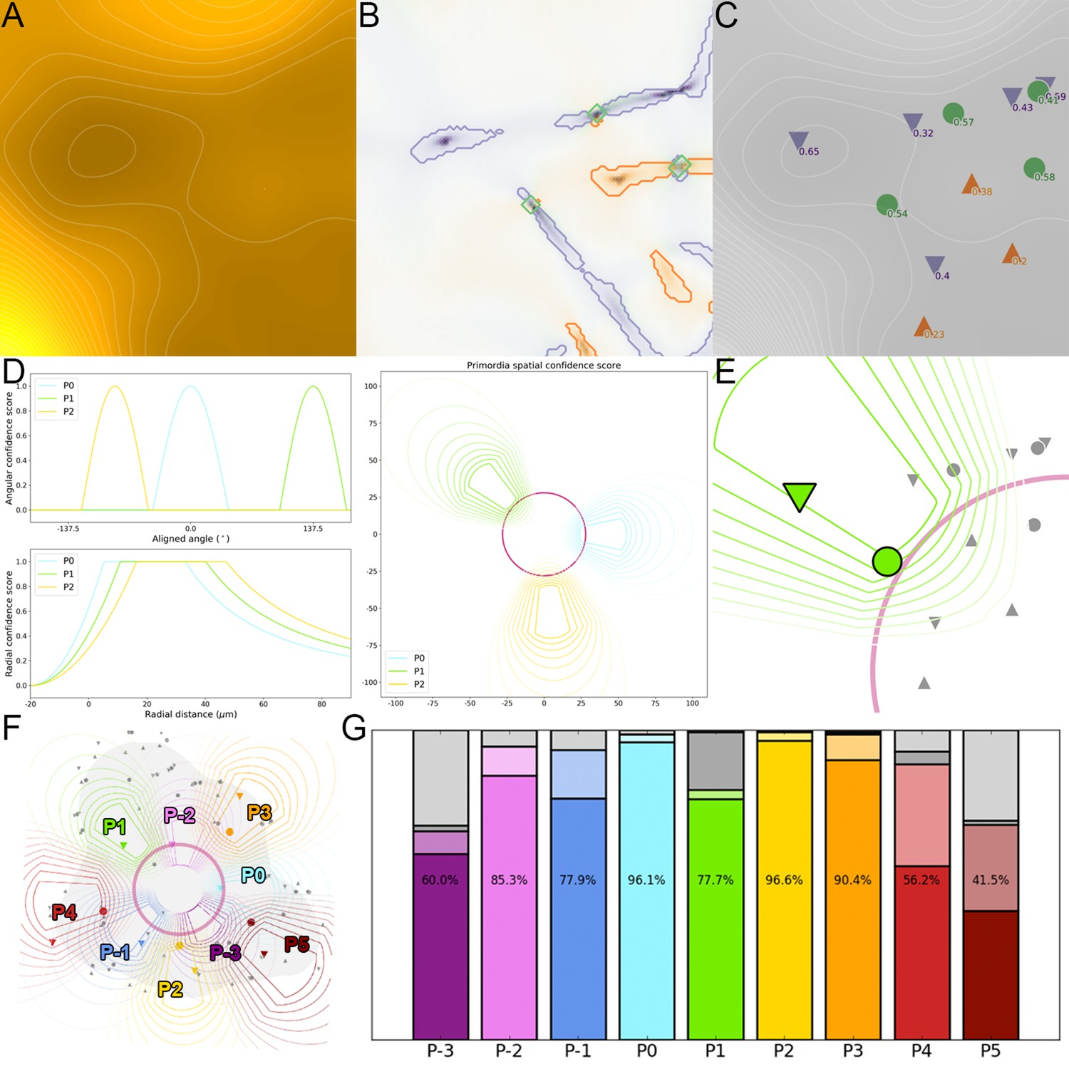
Detection of primordia as extremal regions of auxin.
(A) The auxin distribution forms a landscape where accumulation froms troughs or valleys in the qDII map, whereas depletion forms peaks or ridges. (B). Extremal regions (valleys in purple, ridges in orange and saddles in green) are identified from the qDII map. (C). Each region is associated with a unique spatial position and characterized by a significance score. (D). A geometrical model of primordia distribution is used to compute a confidence score for each extremal region, relatively to each considered primordium rank, depending on its spatial postion. (E). The primordium rank is assigned to the extremal regions with the highest combination of significance and spatial confidence score relatively to (F). This allows to identify the auxin accumulation zoned and the potential auxin depletion zones associated with each primordium in the considered SAM. (G). Comparison of automatically detected auxin extremal points with expertized ones demonstrate a very accurate detection between ranks P0 and P3, with a decreased performance when the features are less well defined (no absolute minimum before P0, several maxima after P4). Color indicates the rank of primordia. Filled color indicates accurate detection, light color indicates correct detection but inaccurate location, dark grey indicates false negatives, light grey indicates false positives.
Appendix 4—figure 1
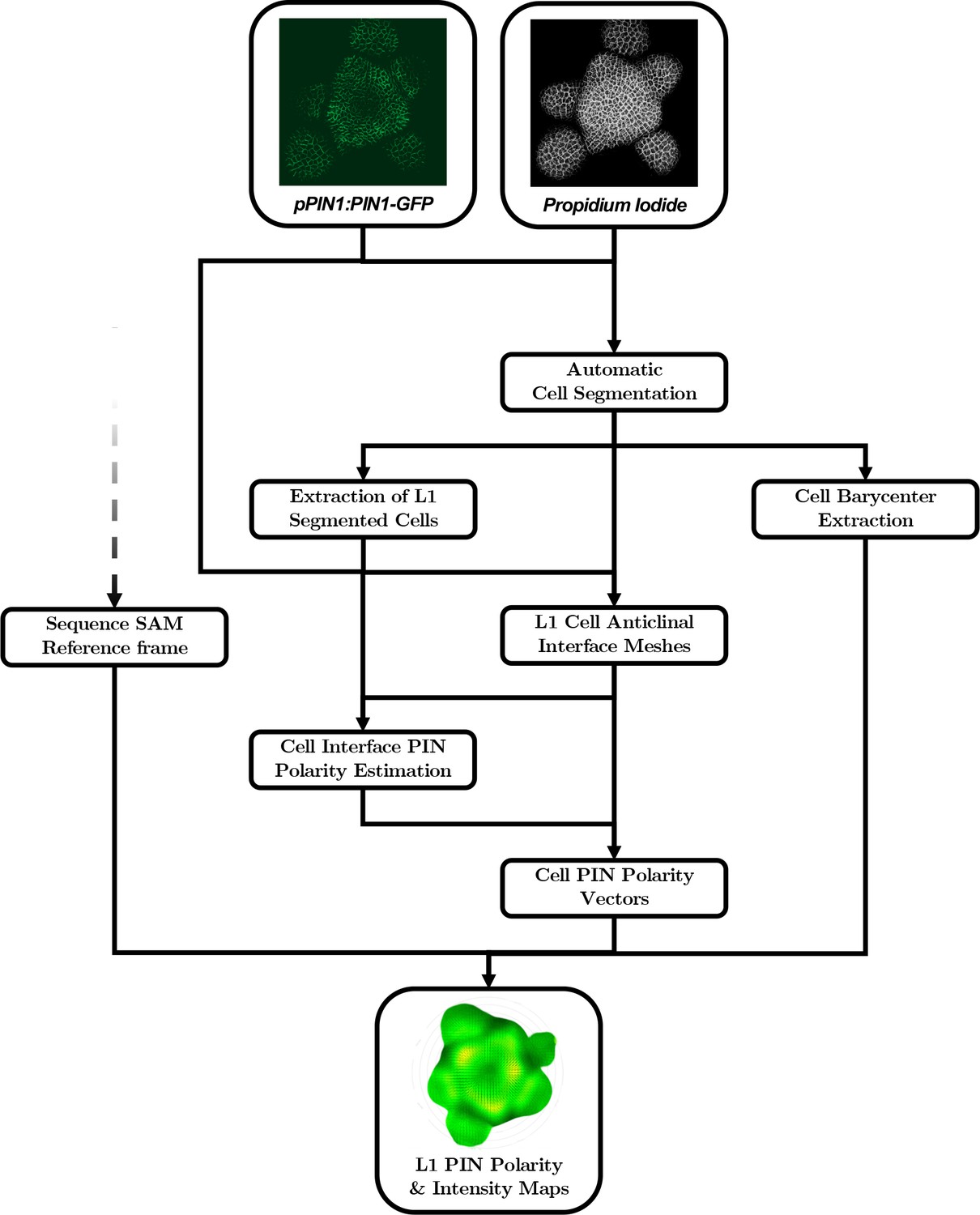
Automatic quantification pipeline for the time-lapse microscopy images of PIN1 auxin efflux carrier.
The quantitative estimation of PIN polarity relies on the analysis of cell wall and membrane-marker images that need to be processed in a different way than nuclei marker images. An alternative automatic pipeline performs the necessary steps, from the segmentation of the cells and the extraction of L1 cell anticlinal interfaces to the quantification of signal distribution at each cell interface and the reconstruction of the polarized cell network.
Appendix 4—figure 2
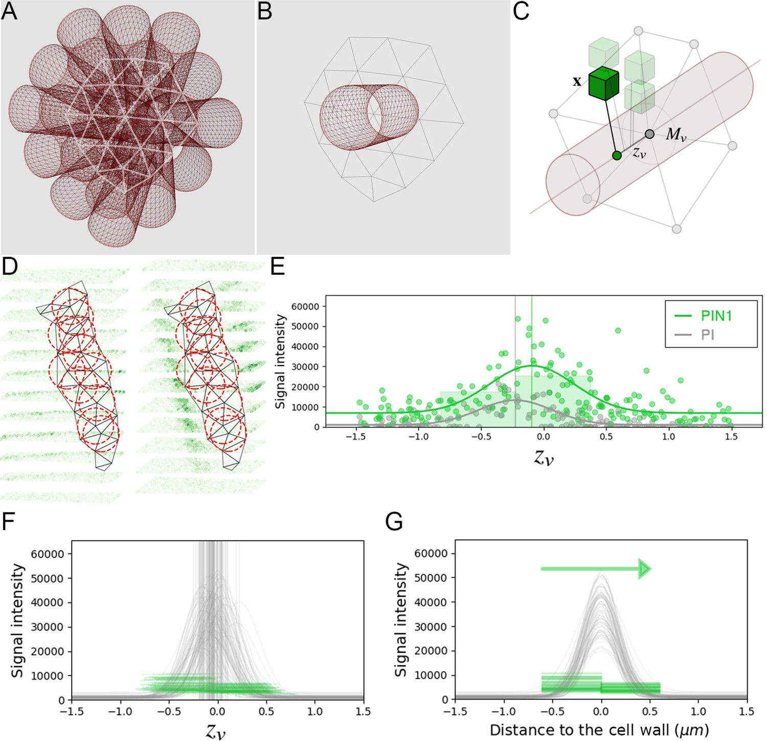
Estimation of PIN polarity at cell interface level.
(A) The triangular mesh representing the cell interface is used to generate a set of 3D cylinders locally orthogonal to the interface and placed at each vertex of the inside of the interface. (B) The radius of the cylinders is close to the typical resolution of the mesh. (C) For each cylinder, all the neighboring image voxels are projected onto its main axis, and kept if within the distance defined by the cylinder radius. Distance of the projected voxel to the interface mesh vertex is used as abscissa for the evaluation of 1d polarity (D) The set of all interface cylinders allow sampling the PIN image signal on either side of the cell-wall at different locations. (E) The 1-dimensional distributions of both PI and PIN image signals along each cylinder are used to locate precisely the cell-wall position and quantify signal levels on either side. (F) PIN levels are estimated left and right of the detected cell-wall abscissa up to a fixed distance of 0.6µ m. (G). Significant difference between left and right distributions of PIN levels across the interface allows deciding for local PIN polarity at the scale of the cell interface.
Appendix 4—figure 3
Evaluation of cell interface PIN1 polarities using manually annotated SRRF images.
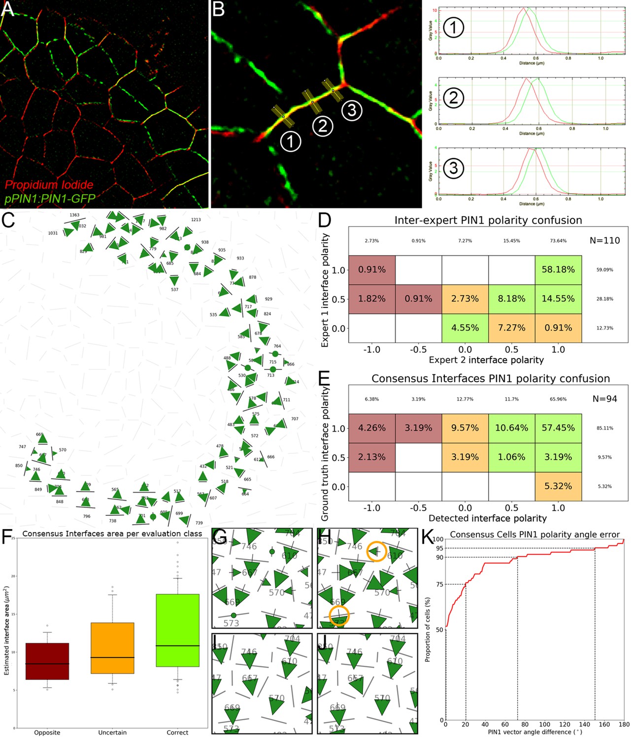
(A) The super-resolution radial fluctuations method produces a 2D image slice with a greatly improved pixel resolution and a less spread-out signal. (B) Using the ImageJ line tool, polarities were manually estimated for each pair of neighbor cells by looking at the relative position of the peaks of PIN1 and PI signals along lines locally orthogonal to the cell interface. In the displayed case, the ground truth polarity value would be -1 as PIN1 lies clearly and consistently to the right of PI. (C) The interfaces on which both experts were in consensus form a set of polarity values that we use as a ground truth to evaluate the results of the automatic method. (D) Comparison of cell interface polarities assigned by the first expert taken as reference (-axis) with the ones assigned by the second expert (-axis). Each cell corresponds to the percentage of annotated interfaces (N = 110) for which expert one assigned the polarity and expert two the polarity . Agreement between experts is represented in green cells (85%), disagreement in dark red cells (4%) and uncertain cases in orange cells (11%). Empty cells correspond to a percentage 0%. (E). Similarly displayed comparison of ground truth polarities taken as reference (-axis) and detected polarities. More than 72% of interfaces have ‘Correct’ predicted polarities (green cells) and less than 10% have ‘Opposite’ polarities (dark red cells). 18% of cells have an ‘Uncertain’ polarity decision (orange cells). (F). The interfaces where errors were made appear to be generally smaller ones. (G–J). Local errors between the ground truth interface polarities (G) and automatically detected ones (H) as those highlighted in orange circles do not necessarily translate into errors between the corresponding polarity vectors integrated at the level of the cells (I and J). (K). Cumulative histogram of cell-level angle errors, showing a very high angular consistency at cell level despite the proportion of interfaces with opposite polarities.
Appendix 5—figure 1
Using spatio-temporal periodicity to extrapolate long-term cellular motions.
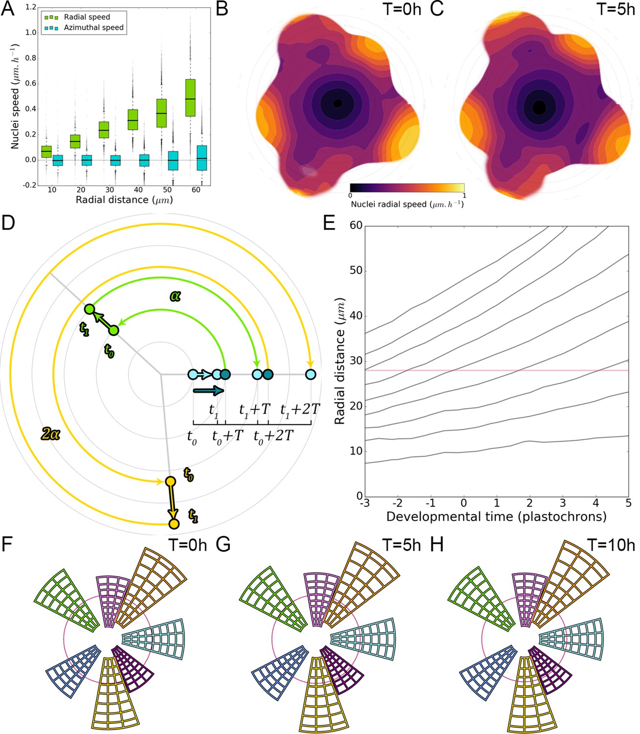
(A). Cellular motion on the L1 is essentially a radial motion towards the periphery of the SAM that accelerates as cells exit the CZ. (B–C). Average 2D maps of L1 local radial cellular speed, computed from image deformations between observations at t = 0 hr and t = 5 hr (B) and t = 5 hr and t = 10 hr (C) ( SAMs). (D). Spatio-temporal periodicity allows estimating cellular motion on several plastochrons by successive rotations: motion at can be used to estimate position at , which can be extrapolated to . By periodicity, radial motion a is equal to radial motion at rotated by one divergence angle , which gives the position at , and so on. (E). The iteration of this process in time allows the reconstruction of long-term radial cellular trajectories that correspond to the average motion of cells over the population over nearly 100 hr. (F–H). These trajectories are used to define spatial domains that reflect cellular motion over time and allow the study of cell-level processes over long durations.
Videos
Video 1
Auxin developmental continuum over nine plastochrons.
Auxin distribution dynamics in the SAM obtained from population averaging and temporal extrapolation. The developmental stage indicated at the top p=n corresponds to the area located on the right. Color code: yellow = low auxin, to black = high auxin.
Tables
Key resources table
| Reagent type (species) or resource | Designation | Source or reference | Identifiers | Additional information |
|---|---|---|---|---|
| Genetic reagent Arabidopsis thaliana | pPIN1:PIN1-GFP (Col-0) | Benková et al., 2003 | ||
| Genetic reagent Arabidopsis thaliana | pCLV3:mCherry-NLS (Col-0) | Pfeiffer et al., 2016 | ||
| Genetic reagent Arabidopsis thaliana | pYUC1-11:GFP (Col-0) | Liu et al., 2016; Robert et al., 2013 | ||
| Genetic reagent (Arabidopsis thaliana) | yuc1 yuc4/+ pDR5rev::GFP (Col-0) | Robert et al., 2013 | ||
| Genetic reagent (Arabidopsis thaliana) | ett-22 (Col-0) | Pekker et al., 2005 | ||
| Genetic reagent (Arabidopsis thaliana) | pid-14 (Col-0) | Huang et al., 2010 | ||
| Genetic reagent Arabidopsis thaliana | pRPS5a:DII-VENUS-N7-p2A-TagBFP-SV40 (Col-0) | This study | qDII | Request to teva.vernoux@ens-lyon.fr |
| Genetic reagent Arabidopsis thaliana | pDR5rev:2x-mTurquoise2-SV40 (Col-0) | This study | Request to teva.vernoux@ens-lyon.fr | |
| Chemical compound, drug | Trichostatin A | Invivogen | met-tsa-1 | 0.005 mM |
| Chemical compound, drug | Indole-3-acetic acid sodium salt | Sigma-Aldrich | I5148 | 0.2, 1.0, 5.0 mM |
| Software, algorithm | RStudio | RStudio Team, 2015 | RRID:SCR_000432 | |
| Software, algorithm | Image J | RRID:SCR_003070 | https://imagej.net | |
| Software, algorithm | NumPy | RRID:SCR_008633 | http://www.numpy.org | |
| Software, algorithm | SciPy | Virtanen et al., 2020 | RRID:SCR_008058 | http://www.scipy.org |
| Software, algorithm | VTK | Schroeder et al., 2006 | RRID:SCR_015013 | http://www.vtk.org |
| Software, algorithm | scikit-image | van der Walt et al., 2014 | http://scikit-image.org | |
| Software, algorithm | sam_spaghetti | This study Cerutti et al., 2020 | https://gitlab.inria.fr/mosaic/publications/sam_spaghetti/ | |
| Other | Propidium iodide solution | Sigma-Aldrich | P4864 | 0.1 mM |
Additional files
-
Supplementary file 1
RNAseq expression of YUCCA genes at the SAM.
- https://cdn.elifesciences.org/articles/55832/elife-55832-supp1-v1.docx
-
Transparent reporting form
- https://cdn.elifesciences.org/articles/55832/elife-55832-transrepform-v1.docx
Download links
A two-part list of links to download the article, or parts of the article, in various formats.
Downloads (link to download the article as PDF)
Open citations (links to open the citations from this article in various online reference manager services)
Cite this article (links to download the citations from this article in formats compatible with various reference manager tools)
Temporal integration of auxin information for the regulation of patterning
eLife 9:e55832.
https://doi.org/10.7554/eLife.55832


