An image-based data-driven analysis of cellular architecture in a developing tissue
Figures

Overview of key steps in our data-driven analysis workflow.
(A) Image data of the tissue of interest are acquired using 3D confocal fluorescence microscopy. Each sample is labeled with a membrane marker to delineate cell boundaries (top) and samples can additionally be labeled with various other markers of interest (bottom, colored). (B) Using an automated image analysis pipeline, single cells are automatically segmented based on the membrane marker to prepare them for analysis, illustrated here by shifting them apart. (C) Next, data extraction takes place to arrive at numerical features representing the cell shapes (yellow) and the various fluorescent protein distributions of additional markers (other colors). (D) Such well-structured data simplify the application of machine learning techniques for data integration, which here is performed based on cell shape as a common reference measurement. (E) A similar strategy can be used to map manually annotated contextual knowledge (top) into the dataset (bottom), in this case specific cell archetypes chosen based on prior knowledge of the tissue's biology. (F) Finally, all of the resulting data are explored and interpreted through various visualizations and statistics.
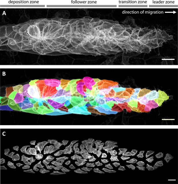
Imaging and automated 3D single-cell segmentation of the pLLP.
(A) Maximum z-projection of a deconvolved 3D volume of the pLLP acquired using the LSM880 AiryScan FAST mode. (B) The same primordium shown with a semi-transparent color overlay of the corresponding single-cell segmentation. (C) Expanded view of the same primordium; individual segmented cells have been shifted apart without being rescaled or deformed, revealing their individual shapes within the collective. Note that the segmentation faithfully recapitulates the diversity of cell shapes within the pLLP, with the exception of fine protrusions. Since the protrusions of follower cells are often impossible to detect against the membranes of the cells ahead of them, we decided not to include fine protrusions in our analysis. All scale bars: 10 μm.
Dynamic View 3D pLLP Stack.
Video of the stack shown in Figure 2A. The slices of the stack are scanned through from bottom to top first, then a maximum z-projection is generated from top to bottom. Scale bar: 10 µm.
Dynamic View of 3D pLLP Segmentation.
Video of the single-cell segmentation shown in Figure 2B. The slices of the stack are scanned through from bottom to top first, then a maximum z-projection is generated from top to bottom. Scale bar: 10 µm.
Dynamic View of 3D Expanded Segmentation.
3D video of expanded segmentation shown in Figure 2C. First, a rotation of the raw data is shown, followed by its expansion based on the single-cell segmentation. Scale bar: 10 µm.
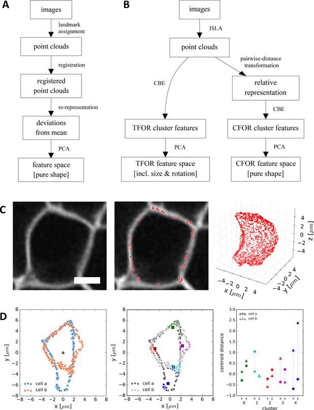
CBE and ISLA for Point Cloud-Based Cell Morphometry.
(A) A classical workflow in landmark-based geometric morphometrics. (B) Adapted workflow for morphometrics of arbitrary fluorescence intensity distributions. See Figure 3—figure supplement 1 for a more detailed version. (C) Illustration of ISLA, our algorithm for conversion of voxel-based 3D images to representative point clouds. Shown are a slice of an input image (left), here a membrane-labeled cell in the pLLP (scale bar: 2 μm), the landmarks sampled from this image (middle), here oversampled compared to the standard pipeline for illustration purposes, and the resulting 3D point cloud (right). (D) Illustration of CBE, our algorithm for embedding point clouds into a feature space. In this 2D mock example, two cells are being embedded based on point clouds of their outlines (left). CBE proceeds by performing clustering on both clouds combined (middle) and then extracting the distances along each axis from each cluster center to the centroid of its ten nearest neighbors (right). Note that the most distinguishing morphological feature of the two example cells, namely the outcropping of cell a at the bottom, is reflected in a large difference in the corresponding cluster's distance values (cluster 4, blue).
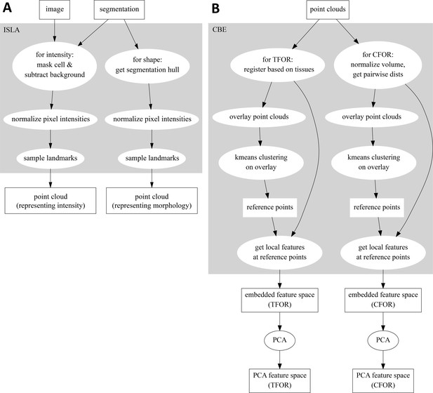
Flowcharts Illustrating the ISLA and CBE Algorithms.
(A) Flowchart of ISLA. To sample from intensity distributions, images are masked by setting voxels outside of the segmentation to zero and a simple background subtraction is performed. To sample from cell shapes, the 1vxl-wide outer shell of the segmentation is set to 1, all other voxels to zero. The resulting image is normalized and used to stochastically sample points for the point cloud. (B) Flowchart of CBE. Input point clouds of cells are either rotated according to a registration across tissues (Tissue Frame Of Reference, TFOR) or are volume-normalized and re-represented as a subset of the pairwise distances between points, removing size and rotational information (Cell Frame Of Reference, CFOR). A representative subset of the resulting clouds is overlaid and k-means clustering is performed on the overlay, yielding a set of common reference points. Finally, features are computed to describe each cell's point cloud relative to these common reference points, resulting in an embedded feature space. This feature space can be transformed with PCA to emphasize relevant variation across the sample population.
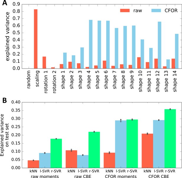
Evaluation of the Expressiveness of CBE Embeddings With and Without Cell Frame of Reference (CFOR) Normalization.
(A) Performance in predicting different generative parameters of point clouds in a synthetic dataset from either a raw or a size- and rotation-corrected (cell frame of reference, CFOR) embedding. As expected, CFOR normalization removes all information on cloud size ('scaling') and orientation ('rotation' 1–2). Interestingly, removing this information allows the regressor to perform far better when it comes to the shape parameters of the point cloud ('shape' 1–14). The 'random' parameter is a random Gaussian distribution and serves as a negative control. The regressor used is a Support Vector Regressor (SVR) with an RBF-kernel. (B) Evaluation of CBE compared to an alternative embedding strategy based on moments. Shown is how well the parameters used to synthetically generate point clouds can be predicted from embeddings of said clouds using different regression models (kNN: k-Nearest Neighbor regressor, l-SVR: linear Support Vector Regressor, r-SVR: RBF-kernel Support Vector Regressor). Black dots indicate results of 3-fold cross-validation, bars indicate the mean. Moments-based embedding is outperformed by CBE in all cases except with linear SVR, where the results are similar.

Analysis of the pLLP's Cellular Shape Space.
(A–B) PCA plots of the tissue frame of reference (TFOR) and an cell frame of reference (CFOR) shape spaces of the pLLP. Each point represents a cell and each color represents a different primordium. Selected example cells are shown as point clouds, illustrating that meaningful properties are encoded in PCs, namely cell orientations (A) and cell sphericity and surface smoothness (B). (C) Explained variance ratios of principal components. (D) t-SNE embedding of the shape space showing the absence of obvious clusters as already seen with PCA in (A–B). Colors indicate different primordia as in (A–B). (E–F) Bigraph visualizations of correlations between principal components of the embedded space (bottom nodes) and a set of engineered features (top nodes). Any edge between two nodes indicates a correlation with Pearson's r > abs(0.3) and stronger edges indicate stronger correlations. A blue hue implies a positive and a red hue a negative correlation. These correlations together with manual inspection as shown in (A–B) allow the biological meaning of embedded features to be determined. (G) Consensus tissue maps of shape space PCs. The contour map represents the local average of PC values across all registered primordia. The small circles show the centroid positions of cells from a single example tissue to aid orientation. The gray bars indicate, from left to right, the deposition zone, follower zone, transition zone, and leader zone. pLLP shape features show varied patterns, including orientation along the D-V axis (TFOR-PC1), characteristic differences between leader and follower cells (TFOR-PC3, CFOR-PC2), and complicated patterns likely arising from the superimposition of different processes (TFOR-PC1).
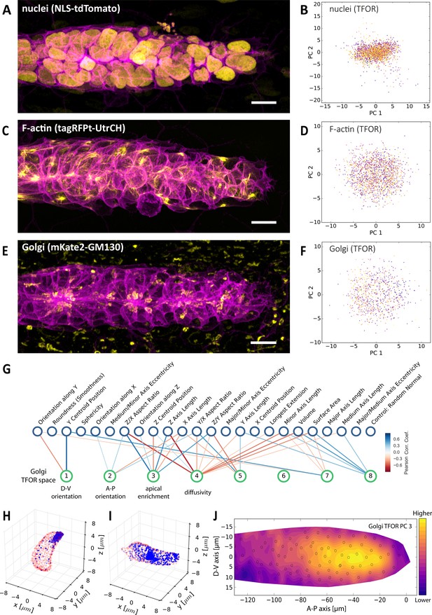
Multi-Channel Imaging, Embedding and Data Integration.
(A, C, E) Maximum z-projections of two-color stacks showing the membrane in magenta and one of three subcellular structures in yellow. (B, D, F) Tissue frame of reference (TFOR) CBE embeddings corresponding to the three structures shown in A, C and E. The different colors of points indicate different primordia. The three structures are nuclei (N = 20, n = 2528) (A–B), F-actin (N = 19, n = 1876) (C–D) and the Golgi apparatus (N = 11, n = 866) (E–F). (G) Bigraph showing correlations between the Golgi's embedded features and our engineered cells shape features (see Supplementary file 2). The first two Golgi TFOR PCs match those found in the cell shape TFOR space (see Figure 4E) whereas PCs 3 and 4 are specific to the Golgi. For technical details see the legend of Figure 4E. (H–I) Point cloud renderings showing the distribution of Golgi signal (blue, membranes in red) in two example cells, one with a high value in the Golgi's TFOR PC 3 (H) and one with a low value (I), illustrating that PC three captures apical enrichment of the Golgi. (J) Consensus tissue map for Golgi PC 3 (apical enrichment), showing increased values behind the leader zone. For technical details see the legend of Figure 4G.
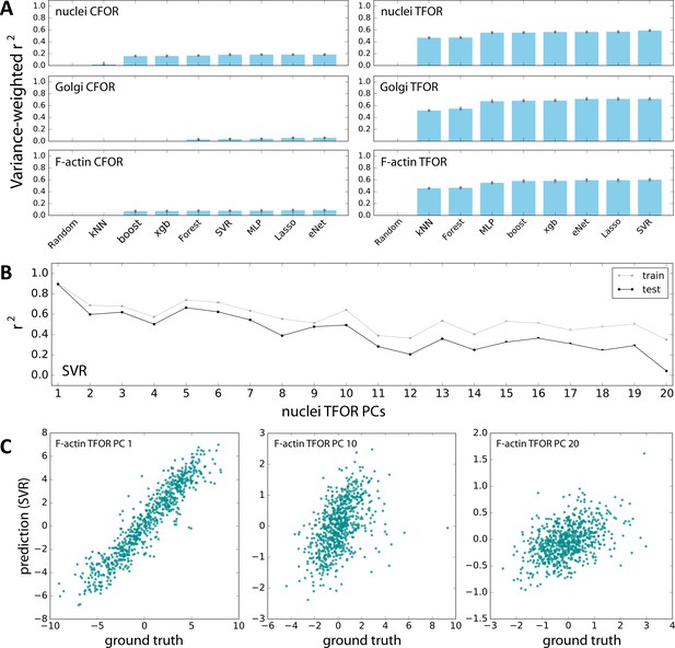
Evaluation of Machine Learning Algorithms for Feature Space Atlas Mapping.
(A) Performance of different algorithms at predicting the embedded feature spaces of different secondary marker channels from embeddings of cell shape. The left column contains predictions from the cell shape CFOR space to subcellular structure CFOR spaces, the right column from cell shape TFOR space to subcellular structure TFOR spaces. Performance is quantified as variance-weighted average of r-squared values across target dimensions. Gray dots are the results from 3-fold cross-validation, blue bars are averages. The algorithms evaluated are a random assignment control (random), k Nearest Neighbors (kNN), the scikit-learn implementation of gradient boosting (boost), xgboost (xgb), random forest regression (forest), support vector regression (SVR), multi-layer perceptrons (MLP), multi-task Lasso regression (Lasso), and multi-task elastic nets (eNet). Note that TFOR predictions work far better than CFOR predictions, which may indicate that pure shape information is insufficient to predict key features of intracellular protein distributions, possibly because information on tissue context is lost. (B) Both for training and prediction, PCA-transformed feature spaces were used. Here, prediction quality is shown for each PC of an example channel, illustrating that high-variance PCs lend themselves to more accurate prediction than low-variance components, as expected given that the latter encode less meaningful variation and more noise. (C) Examples showing the correlation of resulting predictions with ground truths, again illustrating that high-variance PCs (left) can be fitted better than low-variance PCs (right).

pea3 smFISH as an Example of Data Integration Across Imaging Modalities.
(A) Maximum z-projection of a two-color stack of pea3 smFISH (yellow) and the lyn-EGFP membrane marker (magenta). Scale bar: 10 µm. (B) Results of SVR regression on pea3 spot counts using TFOR and CFOR shape features as well as cell centroid coordinates of registered primordia as input. Each blue dot is a cell, the diagonal gray line reflects perfect prediction and blue arrows at the border point to outliers with very high spot counts. On training data, the regressor's explained variance ratio is 0.462 ± 0.011, on previously unseen test data it achieves 0.382 ± 0.019. (C–D) Consensus tissue maps of pea3 expression generated directly from the pea3 smFISH dataset (C) or from the full atlas dataset based on SVR predictions of spot counts (D). Note that the prediction for the entire atlas preserves the most prominent pattern – the front-rear gradient across the tissue – but does not capture the noisy heterogeneity among follower cells observed in direct measurements.
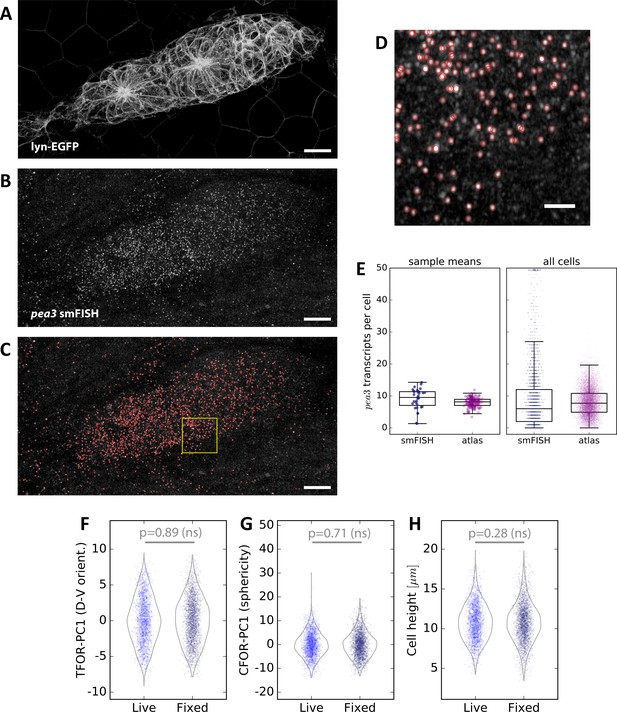
Spot Detection and Cell Shape Embedding for pea3 smFISH Data.
(A–C) Maximum z-projections of a two-color sample showing the lyn-EGFP membrane marker (A), the pea3 smFISH probe (B), and the results of automated spot detection with red rings denoting detection events (C). Scale bars: 10 µm. (D) Zoomed view of the region in the yellow box in (C). Scale bar: 2 µm. (E) pea3 smFISH spot counts for each cell, both from measured data (blue) and from predictions across the entire atlas dataset (purple). The left shows averages across primordia, which closely match those reported previously based on a different spot counting method (Durdu et al., 2014). The individual cell counts on the right show that there is a long tail of cells with extremely high counts, which as one would expect is not captured in the SVR predictions. (F–H) Comparisons of three important cell shape variables between fixed smFISH samples and live samples (here the set of live samples containing only the membrane label; N = 24, n = 2310), showing no significant difference.

Context-Guided Visualization using Morphological Archetypes.
(A) A maximum z-projected example stack with colors highlighting different conceptual archetypes in the pLLP that have been manually annotated. (B) A low-dimensional archetype space resulting from a PCA of the SVC prediction probabilities (with the SVC having been trained on CFOR shape features). Cells are placed according to how similar they are to each archetype, with those at the corners of the tetrahedron belonging strictly to the corresponding archetype and those in between exhibiting an intermediate morphology. (C) Since inter-organ cells are not morphologically distinct enough at this stage (see Figure 7—figure supplement 1), the archetype space can be reduced to 2D without much loss of information. (D) Scatter plots of the 2D archetype space with additional information from the cellular shape space and from the protein distribution atlas superimposed in color. (E–F) Boxplots showing data grouped by predicted archetype labels. This form of grouping allows statistical analysis, showing that leader cells are flatter than any other class of follower cells (E) and that central rosette cells are more spherical than peripheral rosette cells (F). Whiskers are 5th/95th percentiles, p-values are computed with a two-sided Mann-Whitney U-test, and Cohen's d is given as an estimate of effect size.

Evaluation of Morphological Archetype Prediction.
Confusion matrices for SVC archetype classification. The ground truth is based on manual annotation of high-confidence cases. Note that using TFOR features results in slightly better performance than using CFOR features, implying that rotational information and cell size are useful for prediction to some extent. Overall prediction accuracy is high but inter-organ cells are frequently mislabeled, in particular as peripheral cells, indicating that they are morphologically similar at this stage and thus difficult to distinguish based on shape features alone.
Tables
| Reagent type (species) or resource | Designation | Source or reference | Identifiers | Additional information |
|---|---|---|---|---|
| Strain, strain background (Danio rerio) | cldnb:lyn-EGFP | doi:10.1016/j.devcel.2006.02.019 | ZFIN ID:ZDB-TGCONSTRCT-070117–15 | |
| Strain, strain background (Danio rerio) | cxcr4b:NLS-tdTomato | doi:10.1038/nature12635 | ZFIN ID:ZDB-TGCONSTRCT-141217–3 | |
| Strain, strain background (Danio rerio) | Actb2:mKate2-Rab11a | This paper | made with tol2kit, see section ‘Transgenic Fish Lines’ | |
| Strain, strain background (Danio rerio) | LexOP:CDMPR-tagRFPt | This paper | made with tol2kit, see section ‘Transgenic Fish Lines’ | |
| Strain, strain background (Danio rerio) | LexOP:B4GalT1(1-55Q)-tagRFPt; cxcr4b:LexPR | This paper | made with tol2kit, see section ‘Transgenic Fish Lines’ | |
| Strain, strain background (Danio rerio) | atoh1a:dtomato | doi:10.1016/j.ydbio.2010.02.017 | ZFIN ID:ZDB-TGCONSTRCT-100928–4 | |
| Strain, strain background (Danio rerio) | 6xUAS:tagRFPt-UtrCH | This paper | made with tol2kit, see section ‘Transgenic Fish Lines’ | |
| Strain, strain background (Danio rerio) | cxcr4b:LexPR | doi:10.1038/nature13852 | ZFIN ID:ZDB-TGCONSTRCT-170105–4 | LexOP chemically inducible driver line |
| Strain, strain background (Danio rerio) | ETL GA346 | doi:10.1073/pnas.0903060106 | Gal4-UAS driver line | |
| Recombinant DNA reagent | sp6:mKate2-Rab5a (plasmid) | This paper | made with tol2kit, see section ‘Transgenic Fish Lines’ | |
| Recombinant DNA reagent | sp6:mKate2-GM130(rat) (plasmid) | doi:10.1242/jcs.026849 | made with tol2kit, see section ‘Transgenic Fish Lines’ | |
| Sequence-based reagent | CDMPR FOR (D. rerio, full-length) | This paper | PCR primers | GGGGACAAGTTTGTACAAAAAAGCAGGCTGGATGTTGCTGTCTGTGAGAATAATCACT |
| Sequence-based reagent | CDMPR REV (D. rerio, full-length) | This paper | PCR primers | GGGGACCACTTTGTACAAGAAAGCTGGGTCCATGGGAAGTAAATGGTCATCTCTTTCCTC |
| Sequence-based reagent | B4GalT1 FOR (D. rerio, 1-55Q) | This paper | PCR primers | GGGGACAAGTTTGTACAAAAAAGCAGGCTGGATGTCGGAGTCGGTGGGATTCTTC |
| Sequence-based reagent | B4GalT1 REV (D. rerio, 1-55Q) | This paper | PCR primers | GGGGACCACTTTGTACAAGAAAGCTGGGTCTTGTGAATTAACCATATCAGAGATAAATGAAATGTGTCG |
| Sequence-based reagent | Rab5a FOR (D. rerio, full-length) | This paper | PCR primers | GGGGACAGCTTTCTTGTACAAAGTGGCTATGGCCAATAGGGGAGGAGCAACAC |
| Sequence-based reagent | Rab5a REV (D. rerio, full-length) | This paper | PCR primers | GGGGACAACTTTGTATAATAAAGTTGCTTAGTTGCTGCAGCAGGGGGCT |
| Sequence-based reagent | Rab11 FOR (D. rerio, full-length) | This paper | PCR primers | GGGGACAGCTTTCTTGTACAAAGTGGCTATGGGGACACGAGACGACGAATACG |
| Sequence-based reagent | Rab11 REV (D. rerio, full-length) | This paper | PCR primers | GGGGACAACTTTGTATAATAAAGTTGCCTAGATGCTCTGGCAGCACTGC |
| Sequence-based reagent | Quasar 670-conjugated Stellaris smFISH probes | LGC, Biosearch Technologies | smFISH probes | Targeted at D. rerio pea3 gene, see section ‘smFISH: Fixation, Staining and Imaging’ |
| Commercial assay or kit | RNeasy Mini Kit | Qiagen | Cat#:74106 | |
| Commercial assay or kit | QIAshredder | Qiagen | Cat#:79654 | |
| Commercial assay or kit | SuperScript III Reverse Transcriptase | Thermo Fisher Scientifc | Cat#:18080044 | |
| Commercial assay or kit | mMESSAGEmMACHINESP6 Transcription Kit | Thermo Fisher Scientific | Cat#:AM1340 | |
| Commercial assay or kit | MultiSite Gateway Pro | Invitrogen | Cat#:12537 | |
| Chemical compound, drug | LysoTrackerDeep Red | Thermo Fisher Scientific | Cat#:L12492 | |
| Chemical compound, drug | RU486 | Sigma-Aldrich | Cat#:M8046 | |
| Chemical compound, drug | N-phenylthiourea (PTU) | Sigma-Aldrich | Cat#:P7629 | |
| Chemical compound, drug | Tricaine (MESAB) | Sigma-Aldrich | Cat#:A5040 | |
| Software, algorithm | fiji | doi:10.1038/nmeth.2019 | RRID:SCR_002285 | imagej.net/Fiji |
| Software, algorithm | Anaconda | Anaconda, Inc | RRID:SCR_018317 | www.anaconda.com |
| Software, algorithm | python 2.7 | Python Software Foundation | RRID:SCR_008394 | www.python.org/psf |
| Software, algorithm | ISLA | This paper | github.com/WhoIsJack/data-driven-analysis-lateralline (Hartmann, 2020; copy archived at https://github.com/elifesciences-publications/data-driven-analysis-lateralline) | See section ‘Data and Code Availability’ |
| Software, algorithm | CBE | This paper | github.com/WhoIsJack/data-driven-analysis-lateralline | See section ‘Data and Code Availability’ |
Additional files
-
Supplementary file 1
Table of Dataset Composition.
The number of primordia (N) and of segmented single cells (n) that was used in the analysis for each combination of fluorescent labels. The numbers shown do not include the eight samples that were discarded due to low segmentation quality.
- https://cdn.elifesciences.org/articles/55913/elife-55913-supp1-v1.docx
-
Supplementary file 2
Table of Engineered Features.
Brief descriptions of engineered features that were extracted from each segmented cell and used for analysis, in particular to assign biological properties to embedded features extracted with ISLA-CBE.
- https://cdn.elifesciences.org/articles/55913/elife-55913-supp2-v1.docx
-
Transparent reporting form
- https://cdn.elifesciences.org/articles/55913/elife-55913-transrepform-v1.docx


