Figures and data in Molecular determinants of large cargo transport into the nucleus

Figures
Tables
Additional files

5 figures, 3 tables and 3 additional files

Figures

Figure 1 with 1 supplement

Download asset Open asset

A large cargo ‘toolkit’ for nuclear import studies.

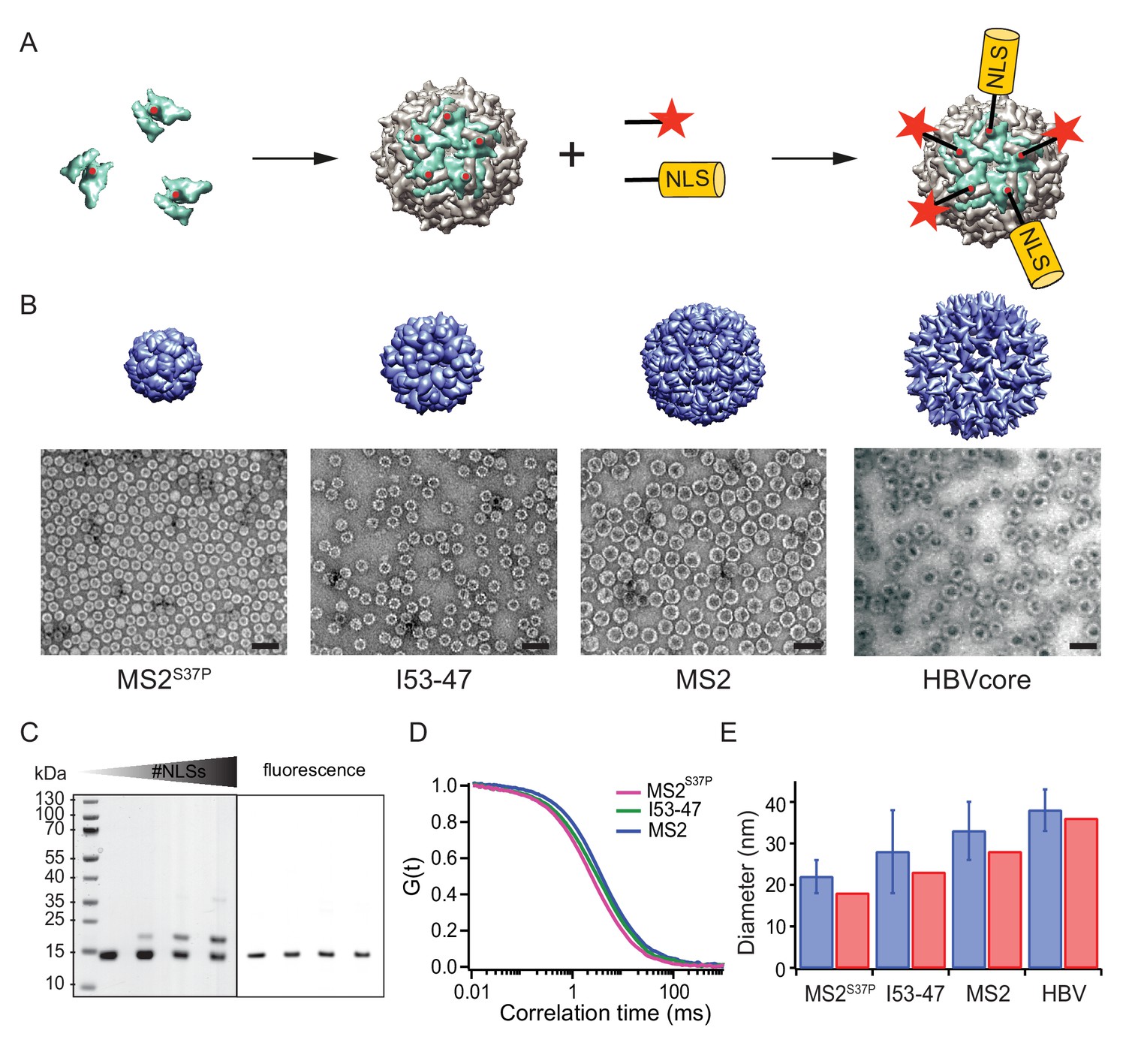
(A) Schematic representation of the mixed labelling reaction with maleimide reactive NLS peptide and maleimide reactive fluorescent dye. The capsid protein, containing a cysteine mutation (in red), self-assembles into a capsid. The purified capsids are then labelled with a mixture of dye and NLS peptide, in different ratios according to the desired reaction outcome. (B) Capsid structures rendered in Chimera (Pettersen et al., 2004) (top) and EM images of the purified capsids (bottom). The scale bar corresponds to 50 nm. (C) SDS-PAGE gel of MS2^S37P samples with increasing number of NLS peptides attached (top band). The lower band corresponds to a capsid protein tagged with dye or no dye, but 0 NLS. The upper band corresponds always to the capsid protein without any dye, but NLS, as evident from the fluorescent scan on the right side. (D) Representative FCS autocorrelation curves for the MS2^S37P, I53-47 and MS2 capsids. The curves were fitted with a diffusion model to calculate the capsid brightness and concentration. (E) DLS quantification of capsid diameters (blue bars) compared with reference values from literature and structural information (red bars).

Figure 1—figure supplement 1

Download asset Open asset

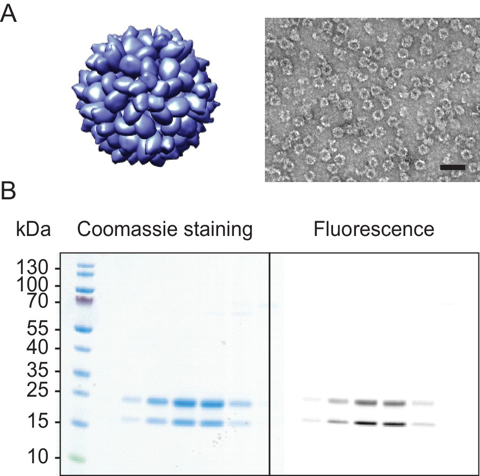
I53-50 capsid.

Analog to main text Figure 1 (A) shows I53-50 capsid structures rendered in Chimera (Pettersen et al., 2004) (left) and EM image of the purified sample (right). The scale bar corresponds to 50 nm. (B) SDS-PAGE gel of I53-50 capsids labelled with Alexa647. The different columns correspond to fractions from the main peak of the size exclusion column. Note, how fluorescent labelling is observed in both chain A (top band) and chain B (bottom band), while the labelling aimed only to label an inserted reactive cysteine residue in chain B. This labelling ambiguity could result in an inaccurate estimate of the #NLSs coupled to the capsid surface, therefore this capsid was excluded from further analysis.

Figure 2 with 2 supplements

Download asset Open asset

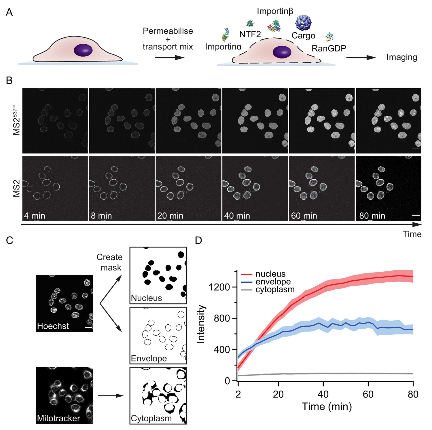
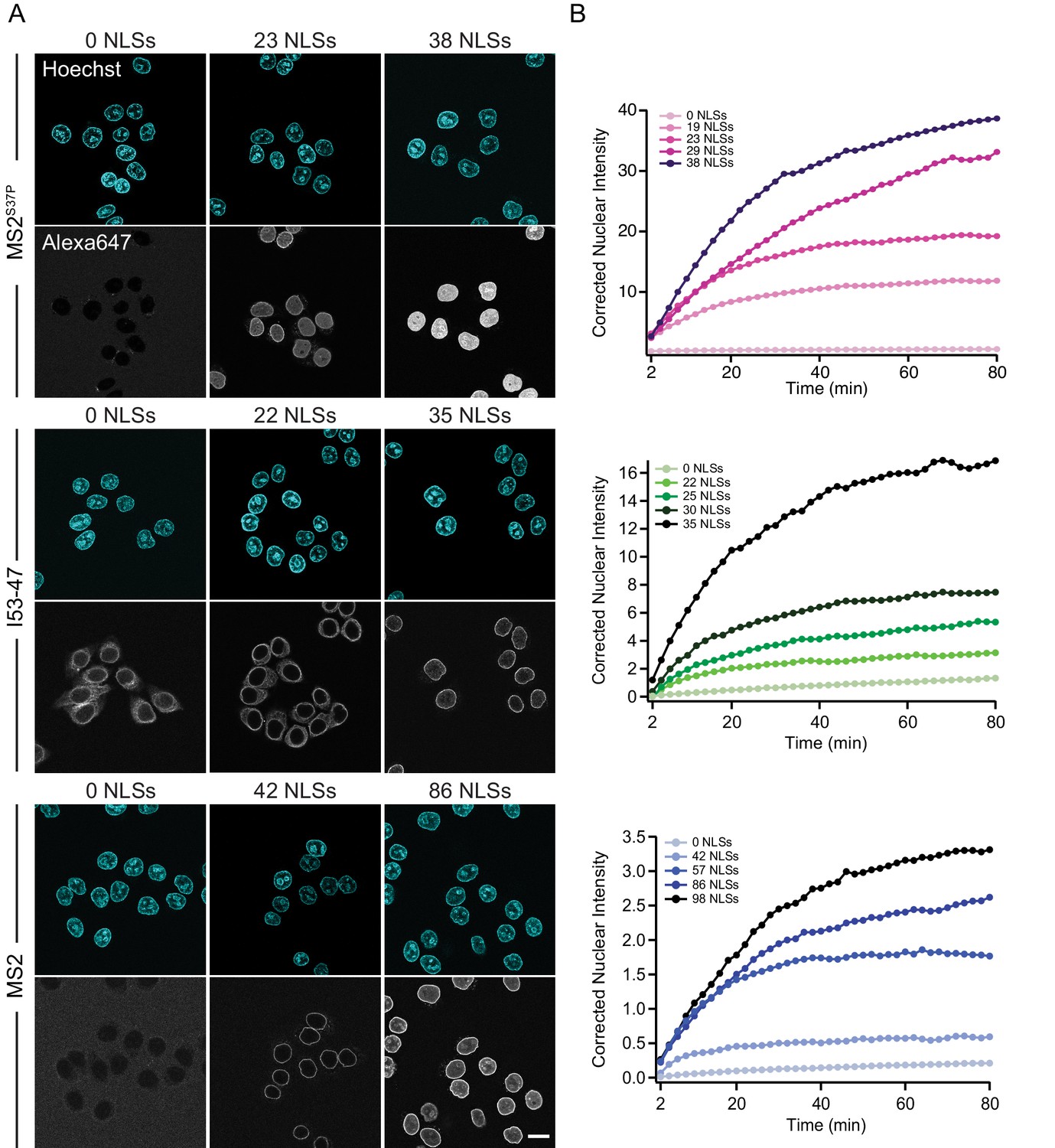
Pipeline for import kinetic experiments.

(A) Scheme of the transport assay experiment: HeLa cells were permeabilised and incubated with a transport mix containing the cargo of interest, nuclear transport receptors and energy. Confocal images were acquired in 12 different areas every 2 min, for 80 min in total. (B) Representative time-lapse snapshots of cargo import (MS2^S37P and MS2 capsids). The scale bar corresponds to 20 μm. (C) Overview of the image analysis pipeline for import kinetics experiments. Two reference stain images (Hoechst and MitoTracker) were segmented and used to generate three masks corresponding to the regions of interest: nucleus, nuclear envelope and cytoplasm. The masks were then applied to the cargo images to calculate the average intensity in the different regions. (D) Representative raw import kinetics traces for the three cellular compartments of interest. Note that imaging starts after 2 min of adding the transport mix to the cells. Curves depict the average fluorescence measured in the different regions; the shaded areas represent the standard deviation over 12 areas.

Figure 2—figure supplement 1

Download asset Open asset

Control experiments in permeabilised cells.

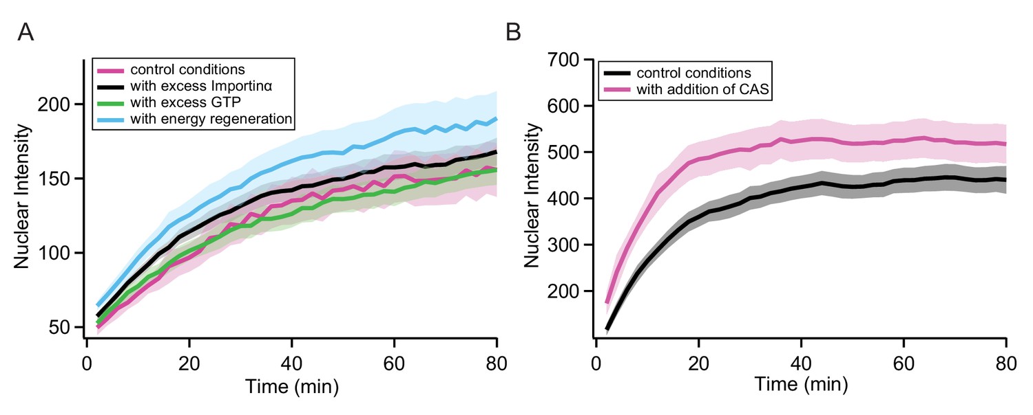
In order to validate the transport assays in permeabilised cells, we performed several control experiments to rule out the possibility that the measured kinetics were for example influenced by depletion of components in the transport mix during the course of the experiment. Panel A shows a comparison of the same MS2^S37P sample measured in normal conditions, with a fivefold excess of Importinα, with a twofold excess of GTP and with addition of an energy regeneration system to the transport mix (0.1 mM ATP, 4 mM creatine phosphate and 20 U/ml creatine kinase). For all cases, capsid import did not change substantially compared to the typical variability in these experiments (the shaded area represents the standard deviation of intensity over 12 different areas acquired). In order to further exclude issues with recycling of transport mix components over time, we purified CAS (the protein responsible for shuttling Importinα back into the cytoplasm [Sun et al., 2013]) and tested its effect on the transport of a MS2^S37P sample with 23 NLSs. As can be seen in panel B, including 1 µM CAS in the transport mix, no major differences in the capsid nuclear import were observed.

Figure 2—figure supplement 2

Download asset Open asset

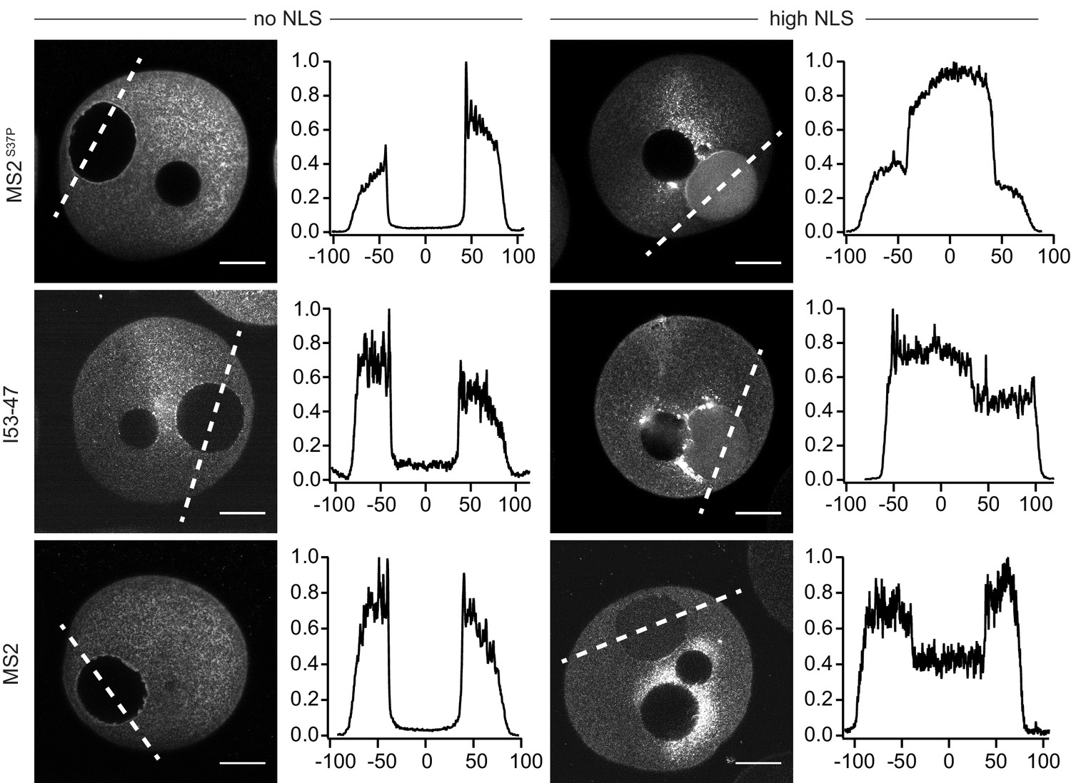
Microinjection of capsids in live starfish oocytes.

Confocal images of starfish oocytes injected with MS2^S37P, I53-47 and MS2 capsids. The plots on the right side correspond to the normalised fluorescence profiles across the nucleus (0 corresponds to the centre of the nucleus, distance in μm, dashed line on the image indicates where the profile is calculated). Note that additional dark areas in the oocyte correspond to oil droplets at the site of injection. For each capsid type, a sample without NLSs was compared with a sample with high #NLSs that showed import in permeabilised cells. Consistent with our results in permeabilised cells with HeLa cells, the efficiency of nuclear accumulation scales with cargo size. Images were taken 1–1.5 hr after injection. Scale bar 50 μm.

Figure 3 with 1 supplement

Download asset Open asset

The import kinetics of large cargoes is tuned by the NLS number.

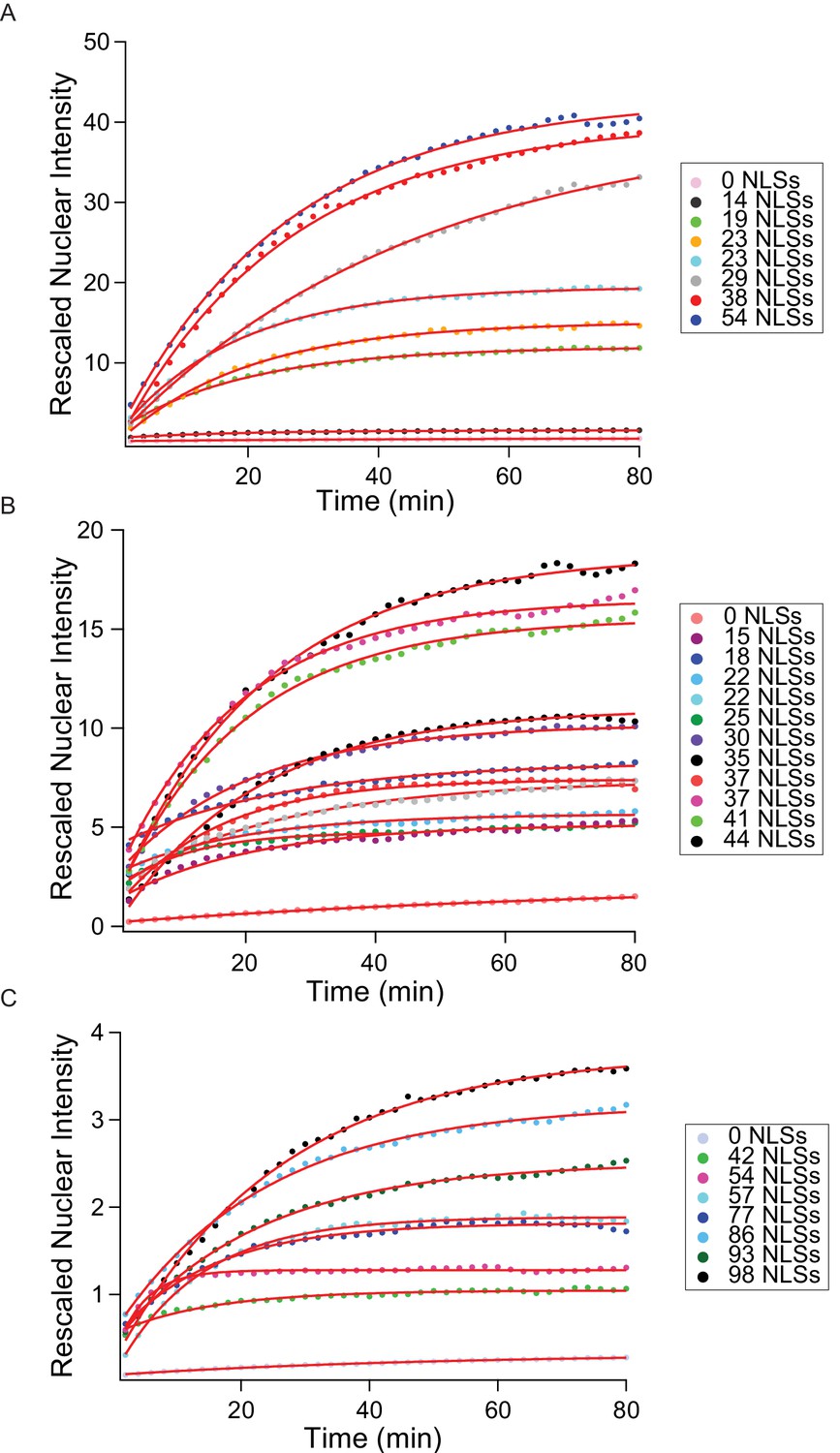
(A) Confocal images of nuclear import of the different large cargoes. Cells were incubated for up to 1.5 hr with capsids tagged with different number of NLS peptides on their surface. All cargoes displayed a distinct NLS-dependent behaviour. The scale bar corresponds to 20 μm. (B) Representative nuclear import traces for the three large cargoes labelled with increasing amount of NLS peptides. The corrected nuclear intensities are obtained by background-subtracting the raw nuclear intensities, scaling them according to capsid brightness (#dyes) estimated from FCS (Table 1) and subtracting the initial offset $A$ determined by the mono-exponential fit, to better compare the import efficiencies. The corrected intensities are proportional to capsid concentration and allow us to compare the import efficiency of the different samples. See Figure 3—figure supplement 1 for the full dataset displayed without offsetting by $A$ and overlaid with mono-exponential fits.

Figure 3—figure supplement 1

Download asset Open asset

Entire import kinetic dataset.

Corresponding to main text Figure 3, here we show all measured kinetics for the MS2^S37P (A), I53-47 (B) and MS2 (C) capsids. The traces represent the average nuclear intensity measured in 12 different areas, background-subtracted and corrected to account for the different sample brightness (#dyes estimated with FCS, see Table 1). Overlaid on top of the traces, we show the mono-exponential fits used to extract the kinetic parameters.

Figure 4

Download asset Open asset

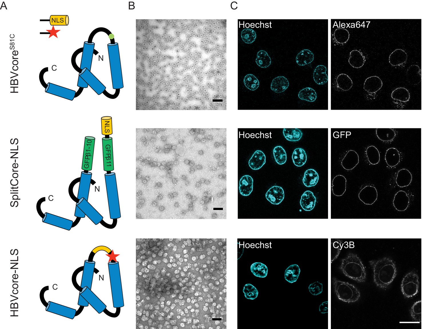
The NLS-engineered Hepatitis B capsid is not imported in the nucleus of permeabilised cells.

Following the same labelling approach as described in Figure 1, HBV capsids with up to 120 NLSs were generated (first row). In order to test capsids with a higher number of NLSs exposed on the surface, we designed two additional versions of the HBV core protein with a direct NLS insertion (total of 240 NLSs). The middle row shows a construct based on the SplitCore-SplitGFP (Walker et al., 2011), where the HBV core protein is split via artificial stop and start codons into two halves and fused to a split-GFP (GFPβ1–10 and GFPβ11), to which we further added an NLS. Once co-expressed, the two core-GFP halves self-assemble into capsid-like particles. The last row shows a construct where the NLS is inserted in the c/e1 epitope loop of the core protein (orange loop) and a cysteine mutation is introduced to perform labelling with a dye (red star). All capsids were targeted to the nuclear envelope but did not give rise to bulk nuclear accumulation in import experiments using permeabilised cells. (A) Schematic representations of the different HBV core protein constructs. (B) EM images of the purified capsids. The scale bar corresponds to 100 nm. (C) Confocal images of capsid import experiments after 1.5 hr. The scale bar corresponds to 20 μm.

Figure 5 with 5 supplements

Download asset Open asset

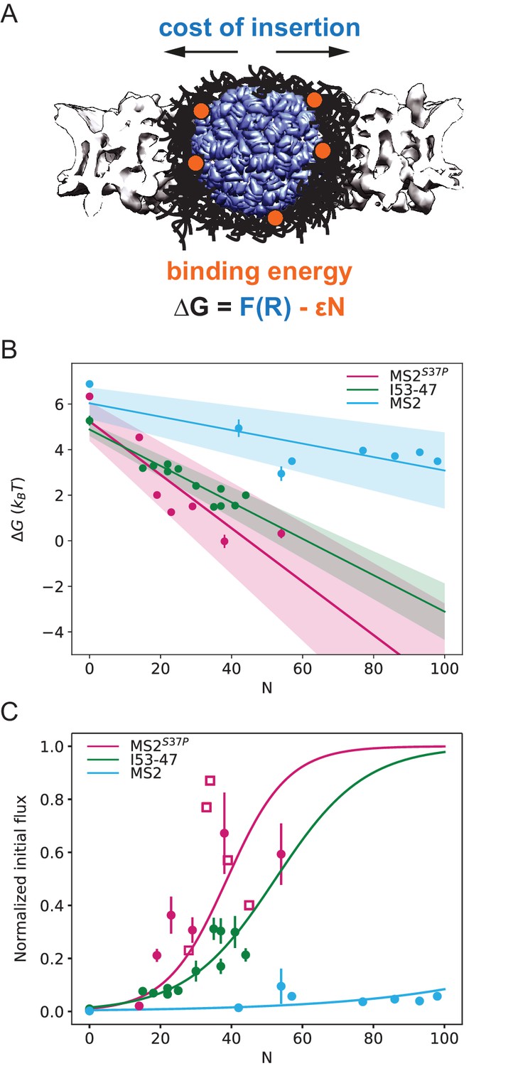
Effect of cargo size and number of NLSs (#NLSs) on import kinetics and biophysical model.

(A) Cartoon of the determinants for large cargo import: the free energy cost of inserting a large cargo into the dense FG Nup barrier must be compensated by the binding to FG Nups via multiple NTRs (binding sites represented in orange, NTRs omitted for simplicity). The NPC scaffold structure is from EMD-8087. (B) Dependence of $Δ G$ on the capsid size and #NLS for $a_{R a n} = 2$ . Shaded regions show one standard deviation of $F (R)$ and $ϵ$ . Fitted values for $F (R)$ and $ϵ$ are shown in Table 2. (C) Initial flux (corresponding to the slope of the kinetic curve at the initial time point) modelled as $J \propto \frac{1}{a_{R a n} + e^{F (R) - ϵ N}}$ overlaid on the (normalised) experimental data (dots). Additional experiments with MS2^S37P capsids containing additional charges are overlaid and shown as squares. Whenever independent biological replicates were available, the initial flux is calculated as an average and shown with the error extracted from the technical replicates (12 areas imaged in each experiment). In Figure 5—figure supplement 5 we show that the uncertainty between different cells imaged in a single experiment captures well the variability of independent experiments.

Figure 5—figure supplement 1

Download asset Open asset

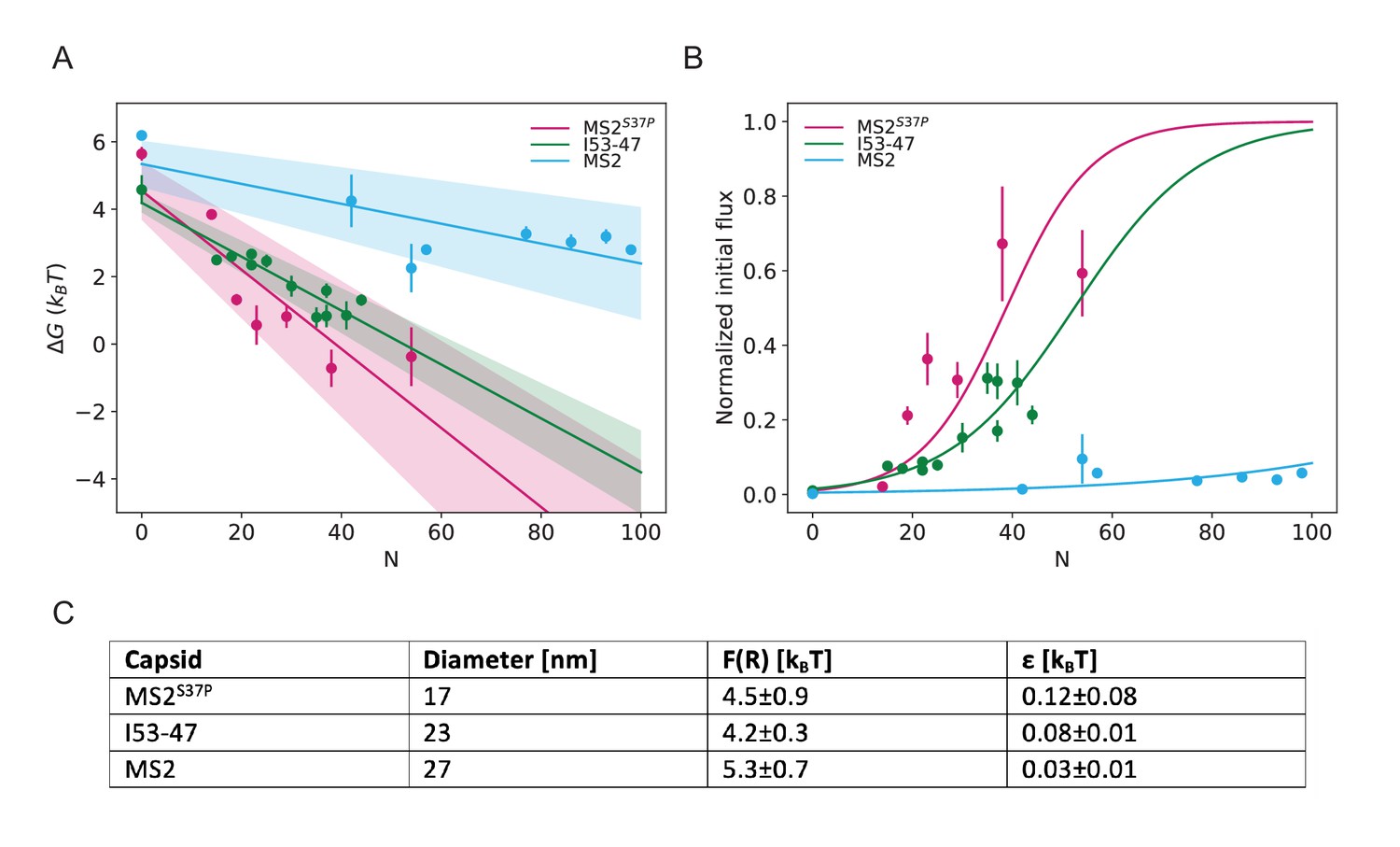
Results from biophysical model with $a_{R a n} = 1$ .

(A) Dependence of $Δ G$ on capsid size and #NLS for $a_{R a n} = 1$ . Shaded regions show one standard deviation of $F (R)$ and $ϵ$ . (B) Initial flux modeled as $J \propto \frac{1}{a_{R a n} + e^{F (R) - ϵ N}}$ overlaid on the (normalised) experimental data. (C) Fitted values for $F (R)$ and $ϵ$ .

Figure 5—figure supplement 2

Download asset Open asset

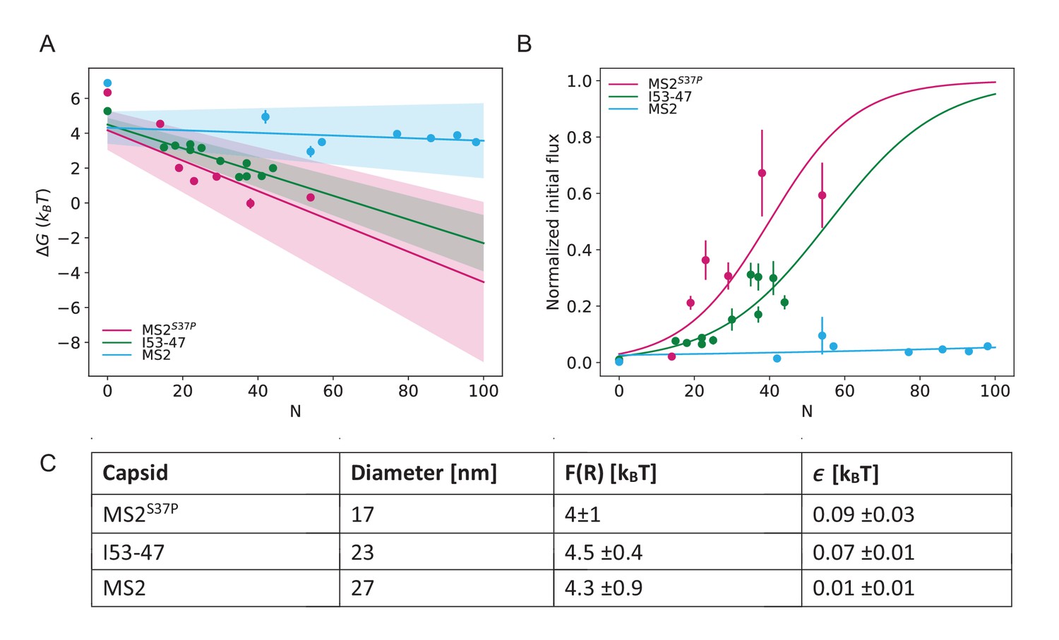
Results from biophysical model where the data point for #NLS=0 is excluded from the fit.

(A) Dependence of $Δ G$ on capsid size and #NLS where the data for #NLS=0 have been excluded from the fitting. (B) The flux determined by the parameters from the fits in (A) overlaid on the initial flux data. (C) Fitted values for $F (R)$ and $ϵ$ , where the data for #NLS=0 have been excluded from the fits.

Figure 5—figure supplement 3

Download asset Open asset

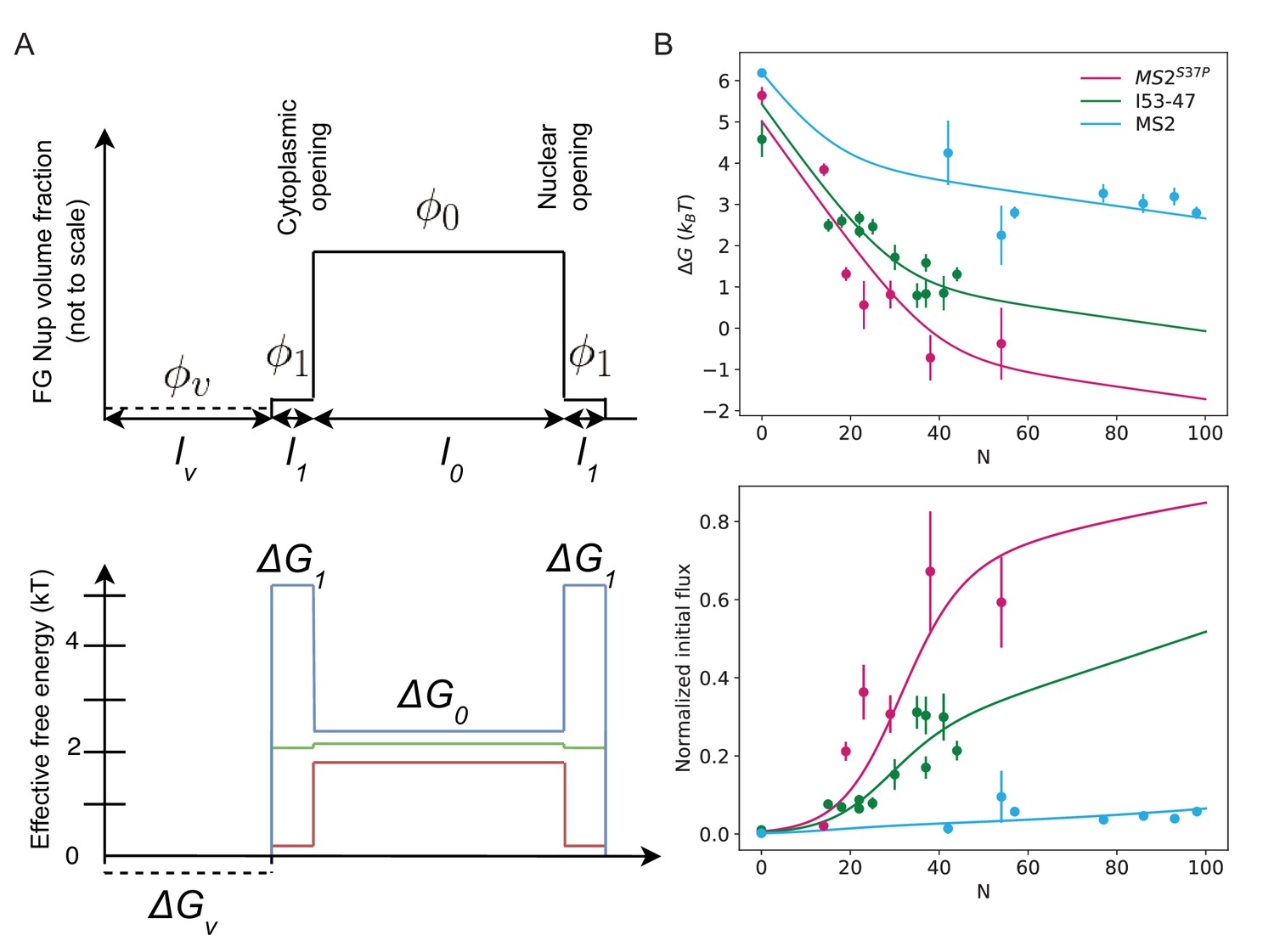
Non-uniform distribution of FG Nups along the pore: theoretical model.

(A) The mathematical model used in the main text corresponds to the simplest case where the density of available NTR binding sites within the FG network is uniform throughout the channel (i.e. $Δ G$ has no dependence on the position along the NPC axis). In reality, accumulating evidence indicates that the density of the FG motifs, and consequently the free energy profile, vary along the pore (Lowe et al., 2010; Tagliazucchi et al., 2013; Tu et al., 2013; Lowe et al., 2015). The top panel depicts one such experimentally motivated density profile, which includes a high density 'barrier' region of high FG Nup density at the centre of the pore ( $ϕ_{0}$ ) (which also increases the cost of insertion in this region [Ghavami et al., 2016; Tagliazucchi et al., 2013]); the low density ( $ϕ_{v}$ cytoplasmic 'docking/vestibule' region with no insertion cost (dashed line), and the transition region between the two with intermediate FG Nup density ( $ϕ_{1}$ ). In this case, the effective free energy in the central region is given by $Δ G_{0} = - ϵ_{0} ϕ_{0} N + F (R, ϕ_{0})$ while in the transition regions the effective free energy is $Δ G_{1} = - ϵ_{0} ϕ_{1} N + F (R, ϕ_{1})$ , where $ϵ_{0}$ is the 'bare' free energy of NTR interaction with an FG motif. The effective free energy in the 'vestibule' is $Δ G_{v} = - ϵ_{0} ϕ_{v} N$ . The initial flux is $J \propto \frac{1}{a_{R a n} + 2 \frac{l_{1}}{l_{T}} e^{Δ G_{1}} + \frac{l_{0}}{l_{T}} e^{Δ G_{0}} + \frac{l_{v}}{l_{T}} e^{Δ G_{v}}}$ where $l_{0}, l_{1}, l_{v}$ are the lengths of the central, peripheral and vestibule regions respectively and $l_{T} = l_{0} + 2 l_{1} + l_{v}$ . Compared with the uniform model in the main text (Figure 5B), $l_{T} e^{Δ G} = 2 l_{1} e^{Δ G_{1}} + l_{0} e^{Δ G_{0}} + l_{v} e^{Δ G_{v}}$ . Bottom panel: Red, green, blue schematically depict effective free energy profiles for N=35 for MS2^S37P, I53-47, MS2 respectively. (B) Top panel: for non-uniform effective free energy, the data for all capsid sizes can be described by a single value of the bare interaction energy $ϵ_{0}$ . Parameter values are: $l_{0}$ = 30 nm, $l_{1}$ = 5 nm, $l_{v} = 20$ nm, $ϕ_{0}$ = 0.01, $ϕ_{1}$ = 0.001, $ϕ_{v} = 0.0005$ , $ϵ_{0}$ = 15.1 $k_{B} T$ . For MS2^S37P: F( $ϕ_{0}$ ) = 5.5 $k_{B} T$ , F( $ϕ_{1}$ ) = 0.9 $k_{B} T$ ; for I53-47: F( $ϕ_{0}$ ) = 5.7 $k_{B} T$ , F( $ϕ_{1}$ ) = 3.3 $k_{B} T$ ; and for MS2 F( $ϕ_{0}$ ) = 6.5 $k_{B} T$ , F( $ϕ_{1}$ ) = 6.0 $k_{B} T$ . We emphasize that this density profile and the parameter values are just one possible combination consistent with the data, and the results are robust with respect to parameter choice. Bottom panel: overlay of the model with the experimental data.

Figure 5—figure supplement 4

Download asset Open asset

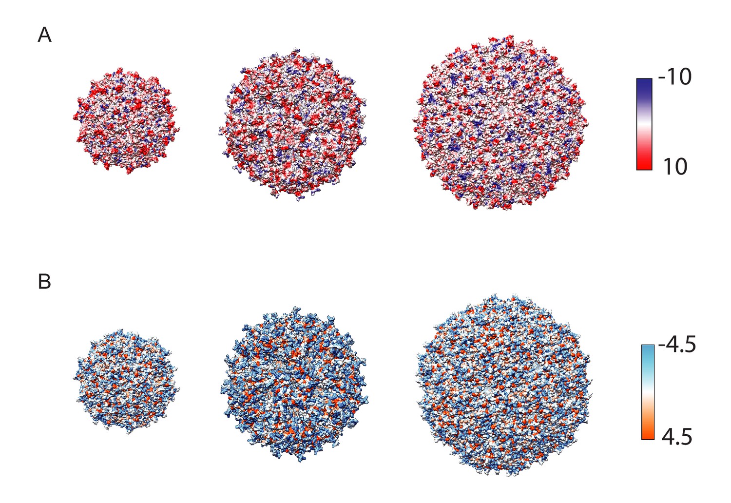
Comparison of large cargo surface properties.

(A) Coulombic surface colouring of the three kinetically investigated capsids, generated in Chimera (Pettersen et al., 2004). The colour scale is in units of *kcal/(mol*e)*, where e is the charge of a single electron. (B) Hydrophobicity surface colouring generated in Chimera, the colour scale refers to units in the Kyte-Doolittle hydrophobicity scale (Kyte and Doolittle, 1982).

Figure 5—figure supplement 5

Download asset Open asset

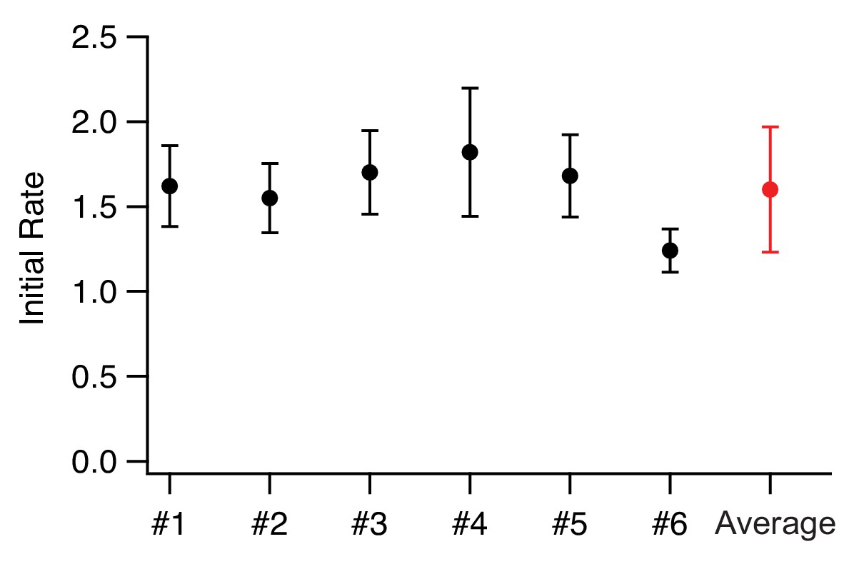
Comparison of biological and technical replicates.

We show here the comparison of six independent biological replicates of the MS2^S37P sample with 38 NLSs. The error bars correspond to the standard deviation between technical replicates (12 different areas images in one experiment). As the technical error already captures the variability between replicates extremely well, we averaged biological replicates when available for the different samples and took the largest technical error as the corresponding uncertainty on the initial flux.

Tables

Table 1

Sample properties and parameters from fits of import kinetics.

Here we list all capsid sample properties (estimated #NLSs and #dyes per capsids), as well as all parameters extracted from fitting the import traces with an inverse exponential $I (t) = A + I_{M A X} (1 - e^{- τ * t})$ . The initial flux is calculated as ${J = I}_{M A X} * τ$ . When different biological replicates were measured for the same sample, the values indicate the average.

	sample	#dyes	#NLSs	A	I_MAX	τ	J	ΔG
MS2^S37P	1	23	0	0.24	0.39	0.022	0.01	6.34
	2	15	14	0.65	0.94	0.054	0.05	4.54
	3	30	19	1.12	12.44	0.041	0.49	2.01
	4	34	23	0.64	16.63	0.053	0.88	1.25
	5	25	29	0.33	28.91	0.022	0.64	1.51
	6	38	38	1.45	43.59	0.037	1.60	−0.02
	7	10	54	2.33	49.76	0.029	1.37	0.32
I53-47	8	24	0	0.18	1.58	0.018	0.03	5.27
	9	30	15	0.80	3.71	0.085	0.32	3.19
	10	31	18	3.81	3.89	0.056	0.22	3.29
	11	36	22	2.34	2.95	0.080	0.23	3.36
	12	16	22	2.01	5.35	0.060	0.32	3.04
	13	31	25	1.83	2.91	0.094	0.27	3.15
	14	6	30	2.27	7.22	0.063	0.45	2.41
	15	3	35	1.18	16.82	0.048	0.81	1.49
	16	8	37	1.21	6.67	0.053	0.35	2.28
	17	3	37	2.16	13.80	0.059	0.81	1.52
	18	10	41	1.13	13.92	0.057	0.79	1.54
	19	8	44	0.31	11.78	0.038	0.45	2.00
MS2	20	50	0	0.07	0.18	0.038	0.01	6.88
	21	38	42	0.47	0.52	0.106	0.05	4.94
	22	58	54	0.19	1.07	0.241	0.26	2.95
	23	44	57	0.07	1.83	0.074	0.13	3.49
	24	52	77	0.47	1.31	0.072	0.09	3.96
	25	61	86	0.55	2.67	0.042	0.11	3.72
	26	57	93	0.38	2.04	0.051	0.10	3.88
	27	54	98	0.27	3.82	0.033	0.12	3.49

Table 2

Parameters from free energy fit.

Fitted values for $F (R)$ and $ϵ$ values, for $a_{R a n} = 2$ . The error corresponds to the standard deviation.

Capsid	Diameter [nm]	F(R) [k_BT]	ϵ [k_BT]
MS2^S37P	17	5.2 ± 0.9	0.12 ± 0.03
I53-47	23	4.9 ± 0.3	0.08 ± 0.01
MS2	27	6.0 ± 0.7	0.03 ± 0.01

Key resources table

Reagent type (species) or resource	Designation	Source or reference	Identifiers	Additional information
Strain, strain background (E. coli)	BL21	Invitrogen/Thermo Fisher Scientific		AI strain
Cell Line (Homo-sapiens)	HeLa Kyoto	Gift from Martin Beck’s Lab	RRID:CVCL_1922
Recombinant DNA reagent	pBAD_MS2_Coat_Protein–(1–393) (plasmid)	This study		Protein expression plasmid for E. coli (MS2)
Recombinant DNA reagent	pET29b(+)_I53–47A.1–B.3_D43C (plasmid)	This study		Protein expression plasmid for E. coli (I53-47)
Recombinant DNA reagent	pBAD_MS2_Coat_Protein–(1–393)_S37P (plasmid)	This study		Protein expression plasmid for E. coli (MS2^S37P)
Recombinant DNA reagent	pET28a2-SCSG-GB1-coreN-GFPβ1–10//NLS-GFPβ11-coreC149H6 (plasmid)	This study		Protein expression plasmid for E. coli (HBV SplitCore)
Recombinant DNA reagent	pBAD-MCS-CoreN-cys-loop-CoreC-TEV-12His (plasmid)	This study		Protein expression plasmid for E. coli (HBV core with cysteine and NLS)
Recombinant DNA reagent	pET28a2-HBc14SH6_S81C (plasmid)	This study		Protein expression plasmid for E. coli (HBV core with cysteine)
Recombinant DNA reagent	pTXB3-12His-Importin beta WT (plasmid)	This study		Protein expression plasmid for E. coli (Impβ)
Recombinant DNA reagent	pBAD-Importα1-FL-InteinCBD-12His (plasmid)	This study		Protein expression plasmid for E. coli (Impα)
Recombinant DNA reagent	pTXB3-NTF2-intein-6His (plasmid)	This study		Protein expression plasmid for E. coli (NTF2)
Recombinant DNA reagent	pTXB3-Ran Human FL-Intein-CBD-12His (plamid)	This study		Protein expression plasmid for E. coli (Ran)
Peptide, recombinant protein	NLS peptide	PSL GmbH		Mal-GGGGKTGRLESTPPKKKRKVEDSAS
Peptide, recombinant protein	NLS peptide with additional charges	PSL GmbH		Mal-DEDED-GGGGKTGRLESTPPKKKRKVEDSAS
Chemical compound, drug	Hoechst	Sigma	B2261	For nuclei labelling
Chemical compound, drug	Mitotracker green	Invitrogen	M7514	For mitochondria labelling
Chemical compound, drug	FITC-Dextran 70 kDa	Sigma	53471	Used for checking nuclear envelope integrity
Chemical compound, drug	Alexa Fluor 647 maleimide	Invitrogen	A20347	Dye for capsid labelling
Software, algorithm	UCSF Chimera	http://www.rbvi.ucsf.edu/chimera/	RRID:SCR_004097
Software, algorithm	Fiji	https://fiji.sc/#	RRID:SCR_002285
Software, algorithm	SymphoTime	PicoQuant	RRID:SCR_016263
Software, algorithm	Igor Pro	Wavemetrics	RRID:SCR_000325
Software, algorithm	Adobe Illustrator CS6	Adobe	RRID:SCR_010279

Additional files

Source code 1 Source ImageJ/Fiji macro to measure nuclear intensities. The code can be executed in either Fiji or ImageJ. It uses the two reference channels (nuclear and mitochondrial staining) to segment the nucleus, nuclear envelope and cytoplasm and measure the cargo fluorescence intensity in these regions for each frame.: https://cdn.elifesciences.org/articles/55963/elife-55963-code1-v1.zip
Download elife-55963-code1-v1.zip
Supplementary file 1 Comparison with bi-exponential fit. We evaluated the appropriateness of a single- vs double-exponential fit to our kinetic data. In this file we report the fit parameters for the double exponential fit with their very high uncertainties and show that their combinations is tightly constrained to values of the mono-exponential fit parameters.: https://cdn.elifesciences.org/articles/55963/elife-55963-supp1-v1.docx
Download elife-55963-supp1-v1.docx
Transparent reporting form: https://cdn.elifesciences.org/articles/55963/elife-55963-transrepform-v1.pdf
Download elife-55963-transrepform-v1.pdf