Receptor-driven, multimodal mapping of cortical areas in the macaque monkey intraparietal sulcus
- Institute of Neuroscience and Medicine (INM-1), Research Centre Jülich, Germany
- Department of Psychiatry, Psychotherapy and Psychosomatics, Medical Faculty, Germany
- C. & O. Vogt Institute for Brain Research, Heinrich-Heine-University, Germany
- JARA-BRAIN, Jülich-Aachen Research Alliance, Germany
Figures
Figure 1
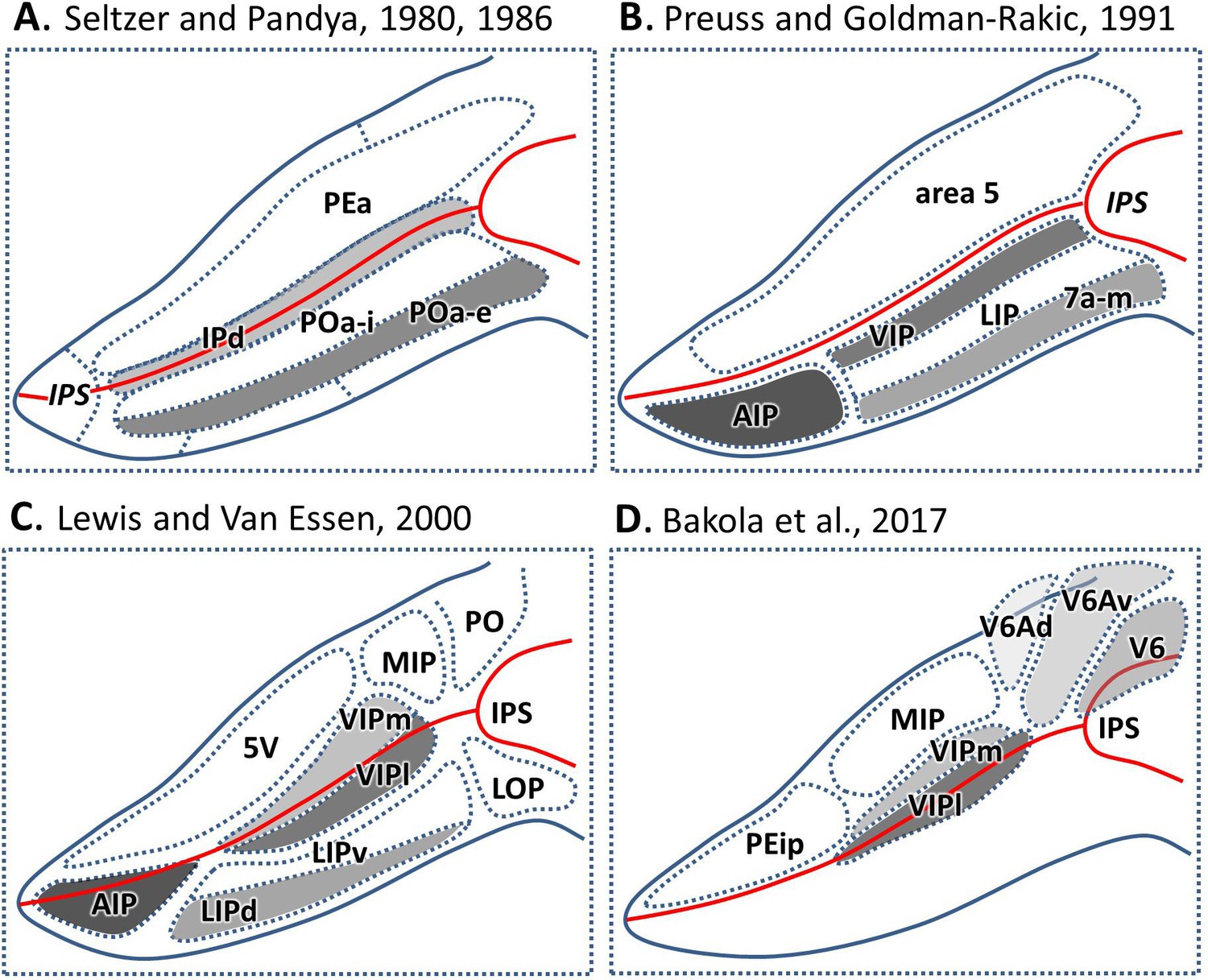
Parcellation of IPS areas in previous studies.
The IPS is unfolded. Blue lines represent the outline of the unfolded IPS, red line represents the fundus of the IPS. (A) Map after Seltzer and Pandya, 1986, Seltzer and Pandya, 1980. (B) Map after Preuss and Goldman-Rakic, 1991. (C) Map after Lewis and Van Essen, 2000a. (D) Map after Bakola et al., 2017. Abbreviations: IPS intraparietal sulcus, IPd intraparietal area (deep), PEa parietal area PEa, POa-i internal part of area POa, POa-e external part of area POa, AIP anterior intraparietal area, VIP ventral intraparietal area, VIPm ventral intraparietal area (medial part), VIPl ventral intraparietal area (lateral part), LIP lateral intraparietal area, LIPd lateral intraparietal area (dorsal), LIPv lateral intraparietal area (ventral), 7a-m, medial part of area 7a, 5V ventral part of area 5, MIP medial intraparietal area, PO parietal-occipital area, LOP lateral occipital parietal, PEip intraparietal part of PE, V6 visual area 6, V6Av visual area 6A (ventral part), V6Ad visual area 6A (dorsal part).
Figure 2

Topography of IPS areas, and at the junction with POS.
Architectonic divisions are shown in a series of coronal cell body-stained sections from the left hemisphere of Macaca mulatta (DP1). The position of each section is highlighted on the lateral view of the left hemisphere. Abbreviations: IPS intraparietal sulcus, POS parietal-occipital sulcus, AIP anterior intraparietal area, VIPm ventral intraparietal area (medial part), VIPl ventral intraparietal area (lateral part), PEipe intraparietal part of PE (external part), PEipi intraparietal part of PE (internal part), LIPd lateral intraparietal area (dorsal), LIPv lateral intraparietal area (ventral), MIPd medial intraparietal area (dorsal), MIPv medial intraparietal area (ventral), V3d dorsal part of visual area 3, V3A visual area 3A, V4d dorsal part of visual area 3, LOP lateral occipital parietal, V6 visual area 6, V6Av visual area 6A (ventral part), V6Ad visual area 6A (dorsal part), PIP posterior intraparietal area.
Figure 3
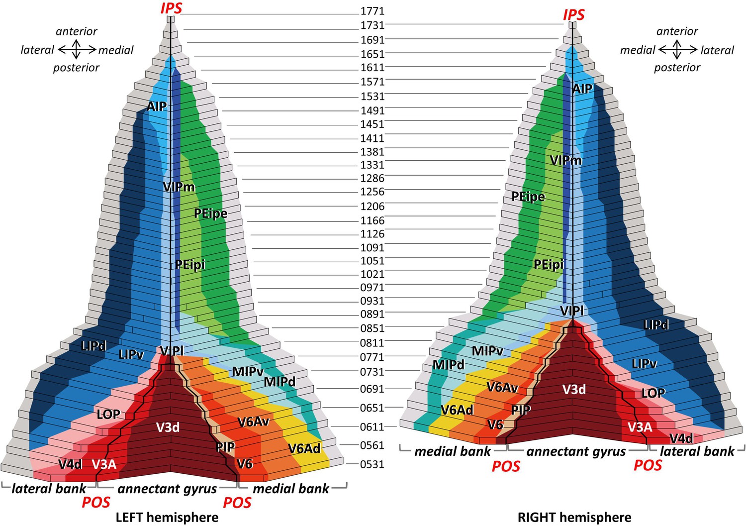
2D cytoarchitectonic flat map of IPS areas in both hemispheres of Macaca mulatta.
Bold lines represent fundi of the intraparietal (IPS) and parieto-occipital (POS) sulci. Arabic numerals mark section numbers. For abbreviations see Figure 2.
Figure 4
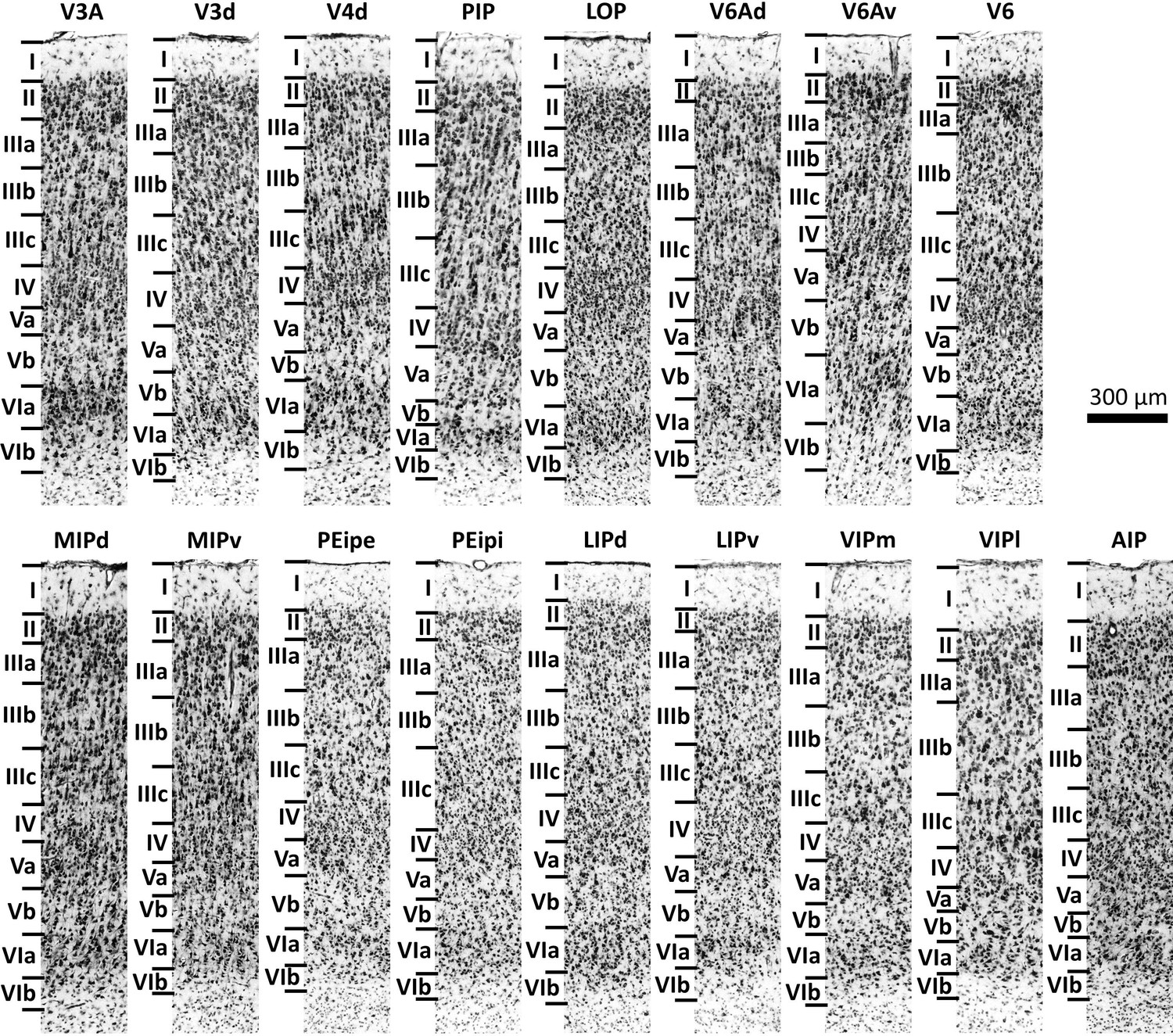
Cytoarchitecture of the 17 IPS areas.
Scale bar 300 μm. Roman numerals indicate cytoarchitectonic layers. For abbreviations, see Figure 2.
Figure 5
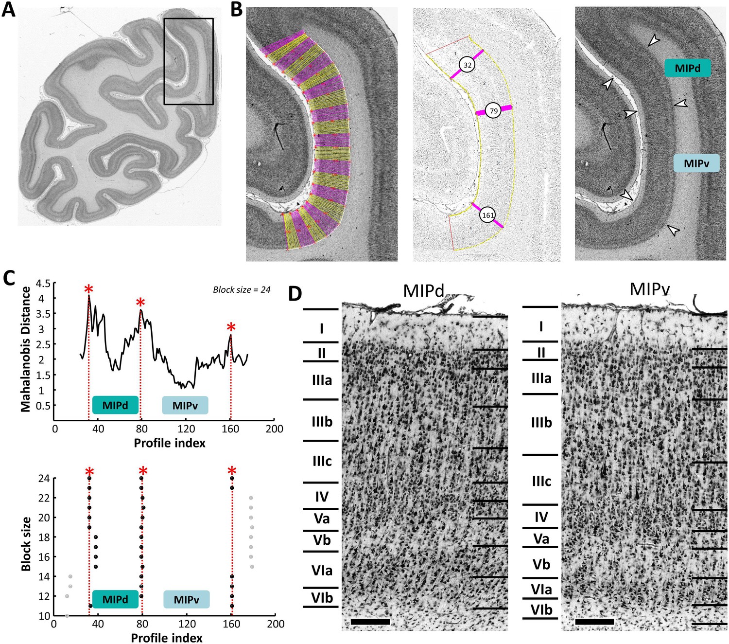
Example of the identification of cytoarchitectonic borders for MIPd and MIPv.
(A) The black box on the overview of a coronal section processed for cell bodies indicates the location of the photomicrograph shown on the right. (B) The cortical ribbon was covered by traverses (from which GLI profiles were extracted) running perpendicular to the cortical layers; color changes between yellow and pink after every 10th traverse (left). Automatic labeling of the positions of the statistically defined borders (at position 32, 79 and 161) (middle). The position of borders of areas MIPd and MIPv as defined by visual inspection are indicated by white arrows in the corresponding image of the cell body stained section (right). (C) Exemplary Mahalanobis distance function depicting the Mahalanobis distances between neighboring blocks of 24 profiles; significant maxima occurred at profile positions 32, 79 and 161, which identify the borders of areas MIPd and MIPv (top). The significant maxima of varying block sizes (ranging from 10 to 24), indicate a consistently occurring border between both areas at profile location 79 (bottom). (D) High-resolution photomicrographs of cytoarchitectonic subdivisions MIPd and MIPv. Scale bar 200 μm. Roman numerals indicate cytoarchitectonic layers. Abbreviations: MIPd medial intraparietal area (dorsal), MIPv medial intraparietal area (ventral).
Figure 6 with 2 supplements
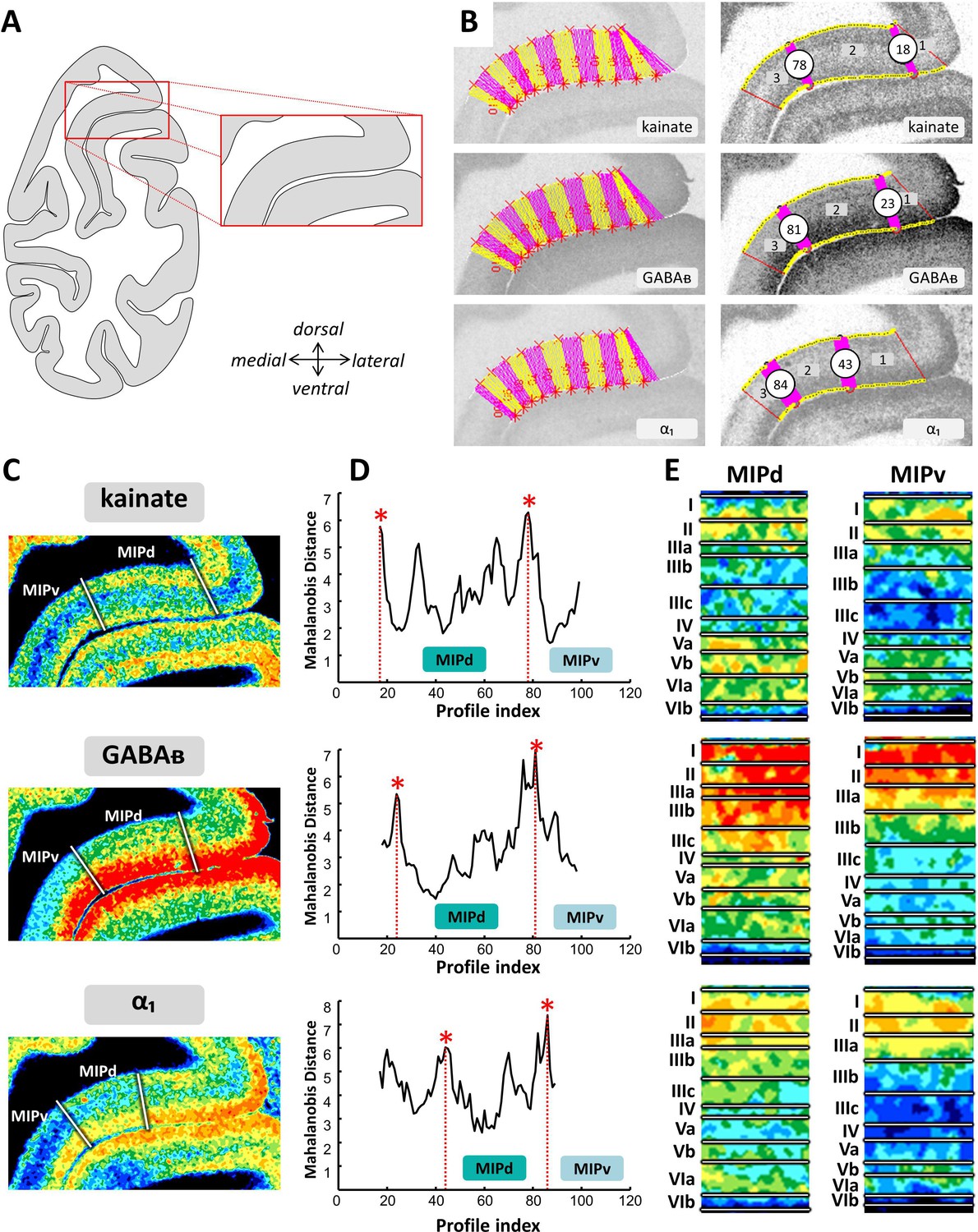
Example of the identification of area MIPd based on receptor distribution patterns.
(A) Schematic representation of an autoradiograph in which the red box indicates the location of the exemplary autoradiographs (kainate, GABAB and α1 receptors) shown in (B) and (C). (B) The cortical ribbon was covered by traverses (from which profiles were extracted) running perpendicular to the cortical layers; color changes between yellow and pink after every 10th traverse (left). Automatic labeling of the positions of the statistically defined borders (right). (C) The position of borders of area MIPd as defined by visual inspection are indicated by white lines in corresponding pseudocolor coded autoardiographs. (D) Exemplary Mahalanobis distance function depicting the Mahalanobis distances between neighboring blocks of 20 profiles; significant maxima occurred at profile positions which coincide with borders for receptor architectonically defined area MIPd. (E) Laminar distribution patterns of corresponding receptors in areas MIPd and MIPv. Roman numerals indicate cytoarchitectonic layers. Abbreviations: MIPd medial intraparietal area (dorsal), MIPv medial intraparietal area (ventral).
Figure 6—figure supplement 1
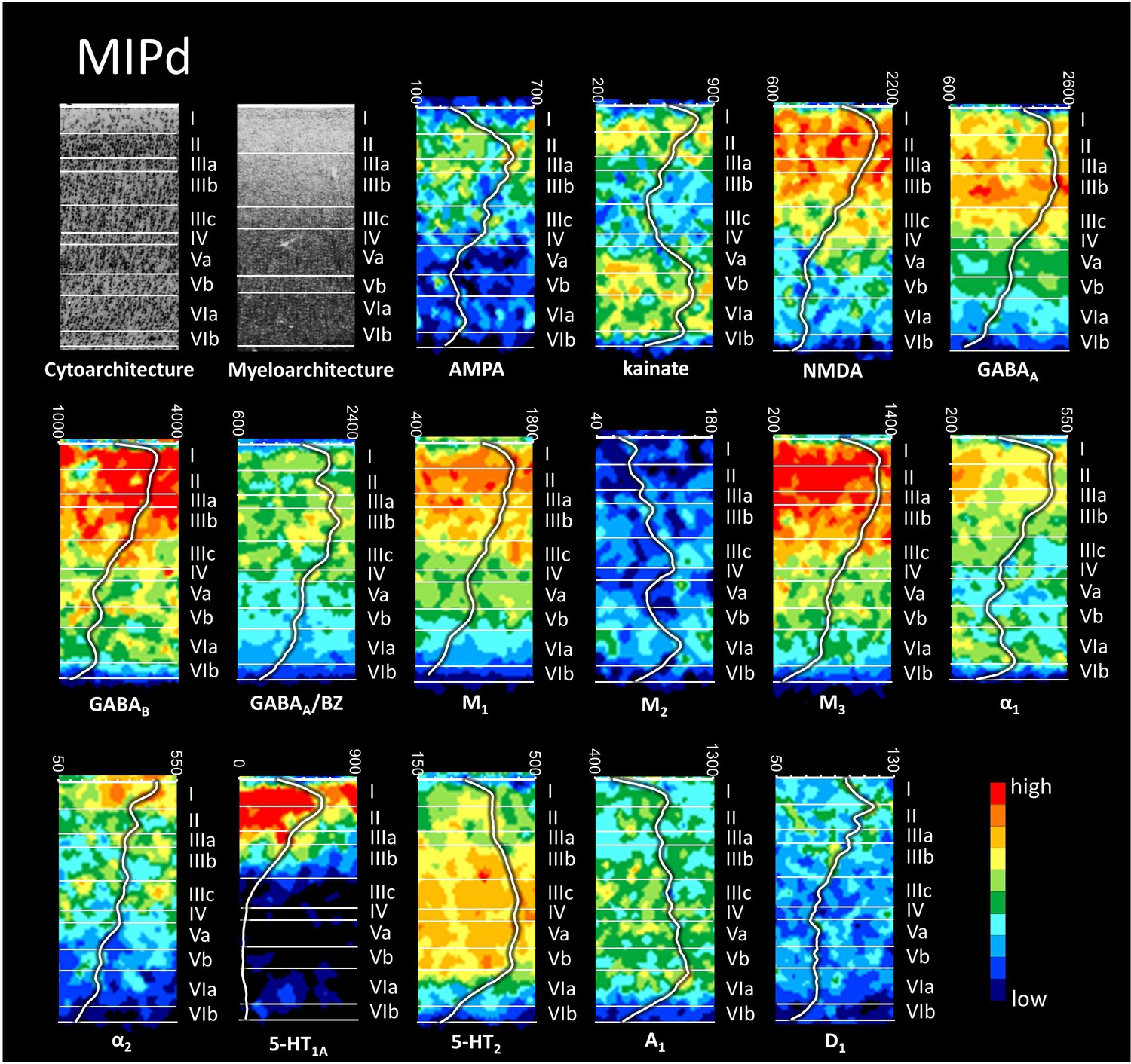
Cyto-, myelo- and receptor architecture of macaque MIPd.
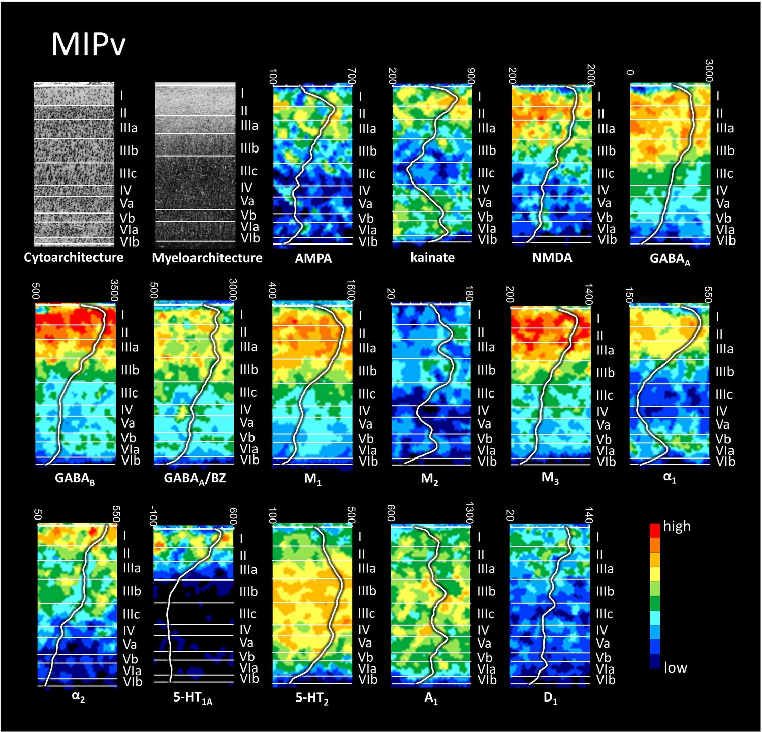
The absolute receptor concentration (in fmol/mg protein) throughout the cortical depth is provided by the profile curve overlaid onto each receptor autoradiograph. Note, that the scale has been optimized for each profile to provide the best visualization of changes in receptor densities throughout the cortical ribbon. Roman numerals indicate cyto- and myeloarchitectonic layers, respectively. Positions of cytoarchitectonic layers were transferred to the neighboring receptor images.
Figure 6—figure supplement 2
Cyto-, myelo- and receptor architecture of macaque MIPv.
For further details, see Figure 6—figure supplement 1.
Figure 7
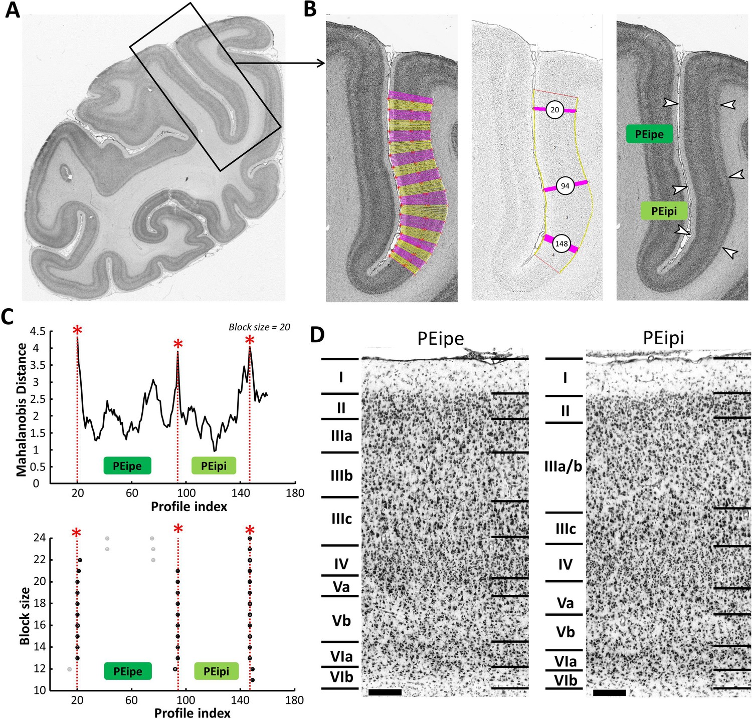
Example of the identification of cytoarchitectonic borders for PEipe and PEipi.
(A) The black box on the overview of a coronal section processed for cell bodies indicates the location of the photomicrograph shown on the right. (B) The cortical ribbon was covered by traverses (from which GLI profiles were extracted) running perpendicular to the cortical layers; color changes between yellow and pink after every 10th traverse (left). Automatic labeling of the positions of the statistically defined borders (at position 20, 94 and 148) (middle). The position of borders of areas PEipe and PEipi as defined by visual inspection are indicated by white arrows in the corresponding image of the cell body stained section (right). (C) Exemplary Mahalanobis distance function depicting the Mahalanobis distances between neighboring blocks of 20 profiles; significant maxima occurred at profile positions 20, 94 and 148, which identify the borders of areas PEipe and PEipi (top). The significant maxima of varying block sizes (ranging from 10 to 24), indicate a consistently occurring border between both areas at profile location 94 (bottom). (D) High-resolution photomicrographs of cytoarchitectonic subdivisions PEipe and PEipi. Scale bar 200 μm. Roman numerals indicate cytoarchitectonic layers. Abbreviations: PEipe intraparietal part of PE (external part), PEipi intraparietal part of PE (internal part).
Figure 8 with 2 supplements
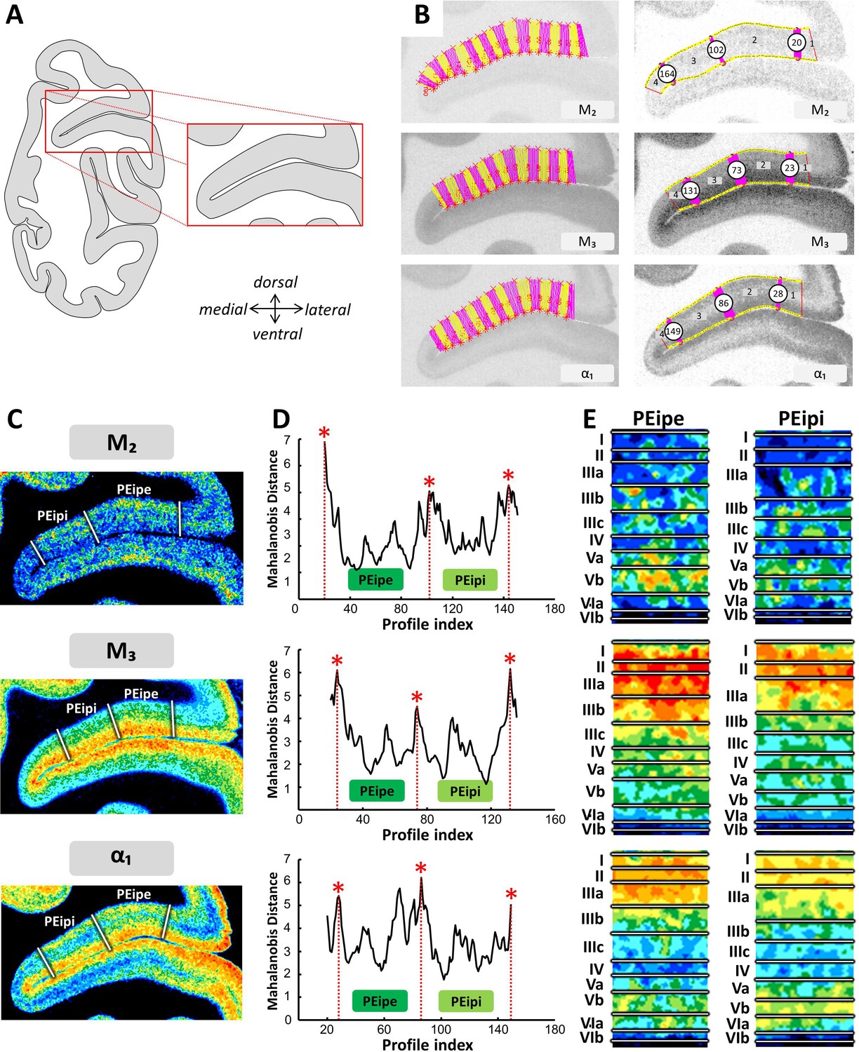
Example of the identification of areas PEipi and PEipe based on receptor distribution patterns.
(A) Schematic representation of an autoradiograph in which the red box indicates the location of the exemplary autoradiographs (M2 M3 and α1 receptors) shown in (B) and (C). (B) The cortical ribbon was covered by traverses (from which profiles were extracted) running perpendicular to the cortical layers; color changes between yellow and pink after every 10th traverse (left). Automatic labeling of the positions of the statistically defined borders (right). (C) The position of borders of areas PEipi and PEipe as defined by visual inspection are indicated by white lines in corresponding pseudocolor coded autoardiographs. (D) Exemplary Mahalanobis distance function depicting the Mahalanobis distances between neighboring blocks of 20 profiles; significant maxima occurred at profile positions which coincide with borders for receptor architectonically defined areas PEipi and PEipe. (E) Laminar distribution patterns of corresponding receptors in areas PEipi and PEipe. Roman numerals indicate cytoarchitectonic layers. Abbreviations: PEipe intraparietal part of PE (external part), PEipi intraparietal part of PE (internal part).
Figure 8—figure supplement 1
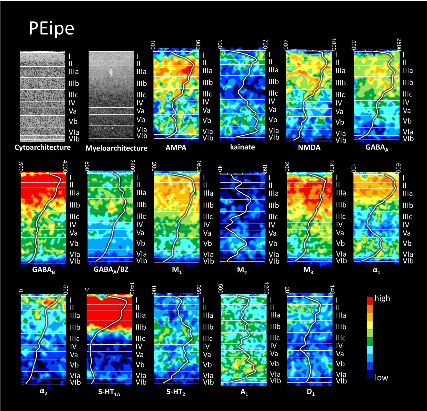
Cyto-, myelo- and receptor architecture of macaque PEipe.
For further details, see Figure 6—figure supplement 1.
Figure 8—figure supplement 2
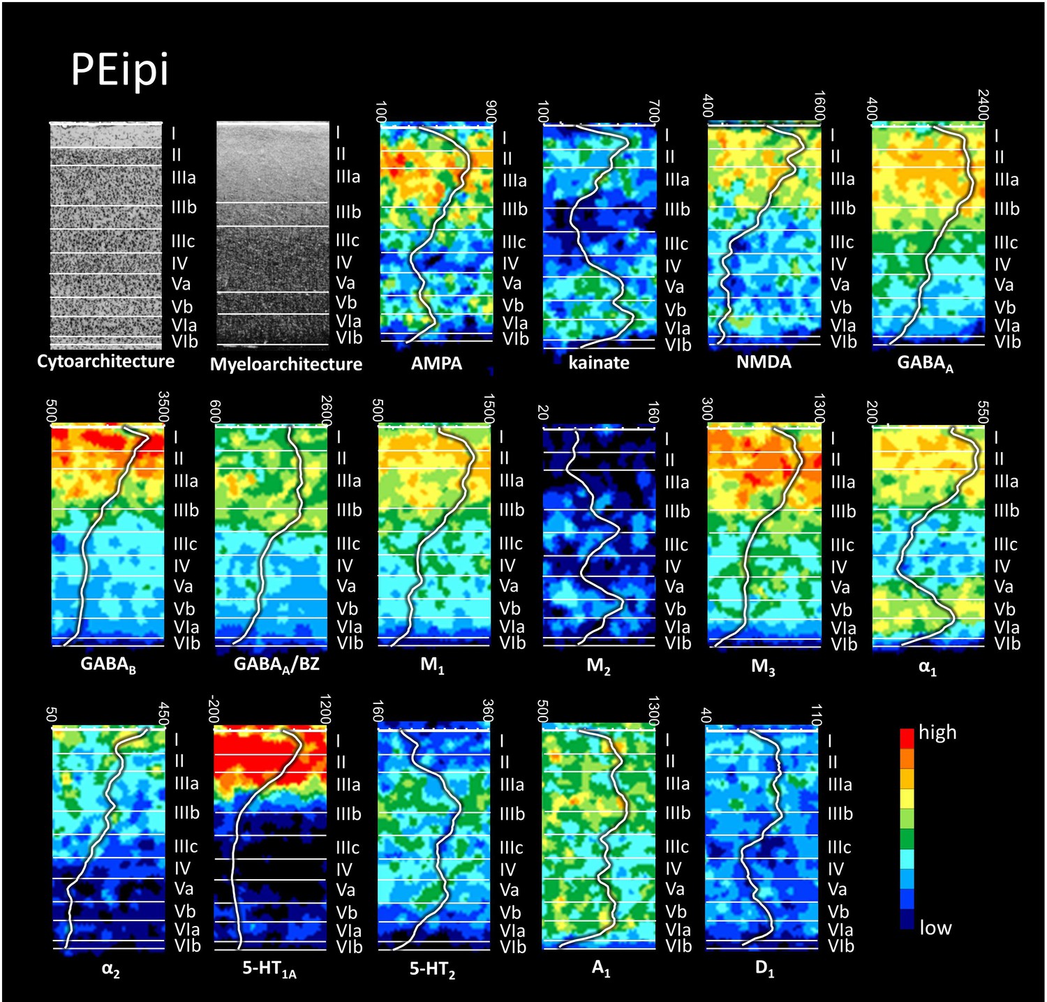
Cyto-, myelo- and receptor architecture of macaque PEipi.
For further details, see Figure 6—figure supplement 1.
Figure 9
Myeloarchitecture of areas of the IPS.
Coronal sections through four rostro-caudal levels of a macaque hemisphere showing the myeloarchitecture of the IPS. For abbreviations, see Figure 2.
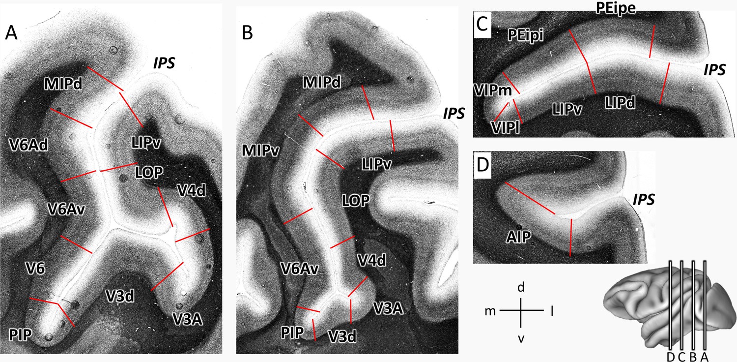
Figure 10 with 4 supplements

Example of receptor distribution patterns in the IPS.
Coronal sections through four rostro-caudal levels of a macaque hemisphere showing exemplary receptor distribution patterns in the IPS. Receptor distribution patterns illustrated for all 15 receptors are shown in Figure 10—figure supplements 1–4. The borders between the IPS areas (red lines) are charted on the pseudocolor-coded autoradiographs. The color bar beneath each autoradiograph indicates receptor concentrations by the different colors, from black for low to red for high concentrations (fmol/mg protein). For abbreviations, see Figure 2.
Figure 10—figure supplement 1
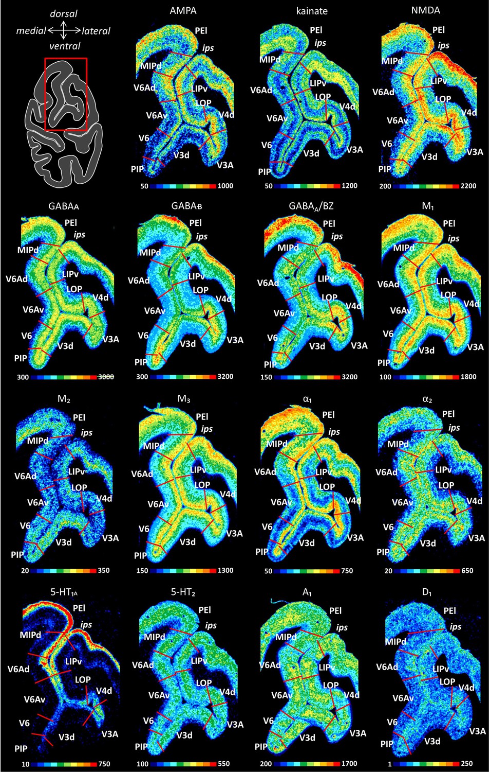
Receptor distribution patterns in the junction of the IPS and POS.
Receptor distribution patterns in areas MIPd, V6Ad, V6Av, V6, V3d, V3A, V4d, LOP and LIPv illustrated for 15 receptors studied. The borders between IPS areas (red lines) are charted on the pseudocolor-coded autoradiographs. The color bar beneath each autoradiograph indicates receptor concentrations by the different colors, from black for low to red for high concentrations (fmol/mg protein). For abbreviations, see Figure 2. Red box on the left section indicates the location of the region of interest.
Figure 10—figure supplement 2
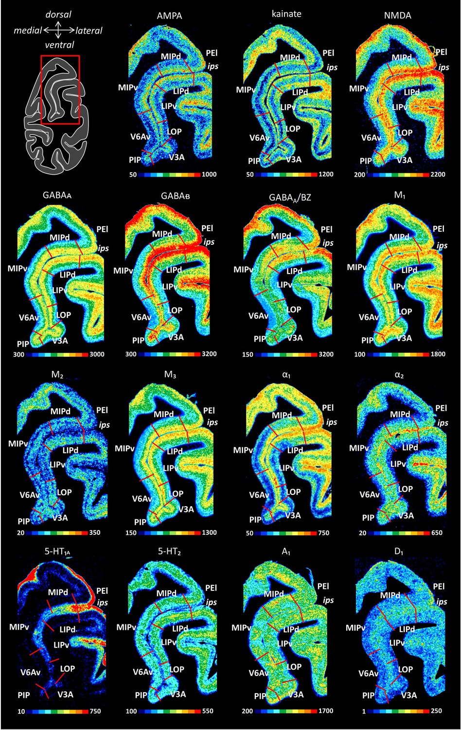
Receptor distribution patterns in the caudal IPS.
Receptor distribution patterns in areas MIPd, MIPv, V6Av, PIP, V3d, V3A, LOP, LIPv and LIPd illustrated for the 15 receptors studied. For further details, see Figure 10—figure supplement 1.
Figure 10—figure supplement 3

Receptor distribution patterns in the middle portion of the IPS.
Receptor distribution patterns in areas PEipe, PEipi, VIPm, VIPl, LIPv and LIPd illustrated for the 15 receptors studied. For further details, see Figure 10—figure supplement 1.
Figure 10—figure supplement 4
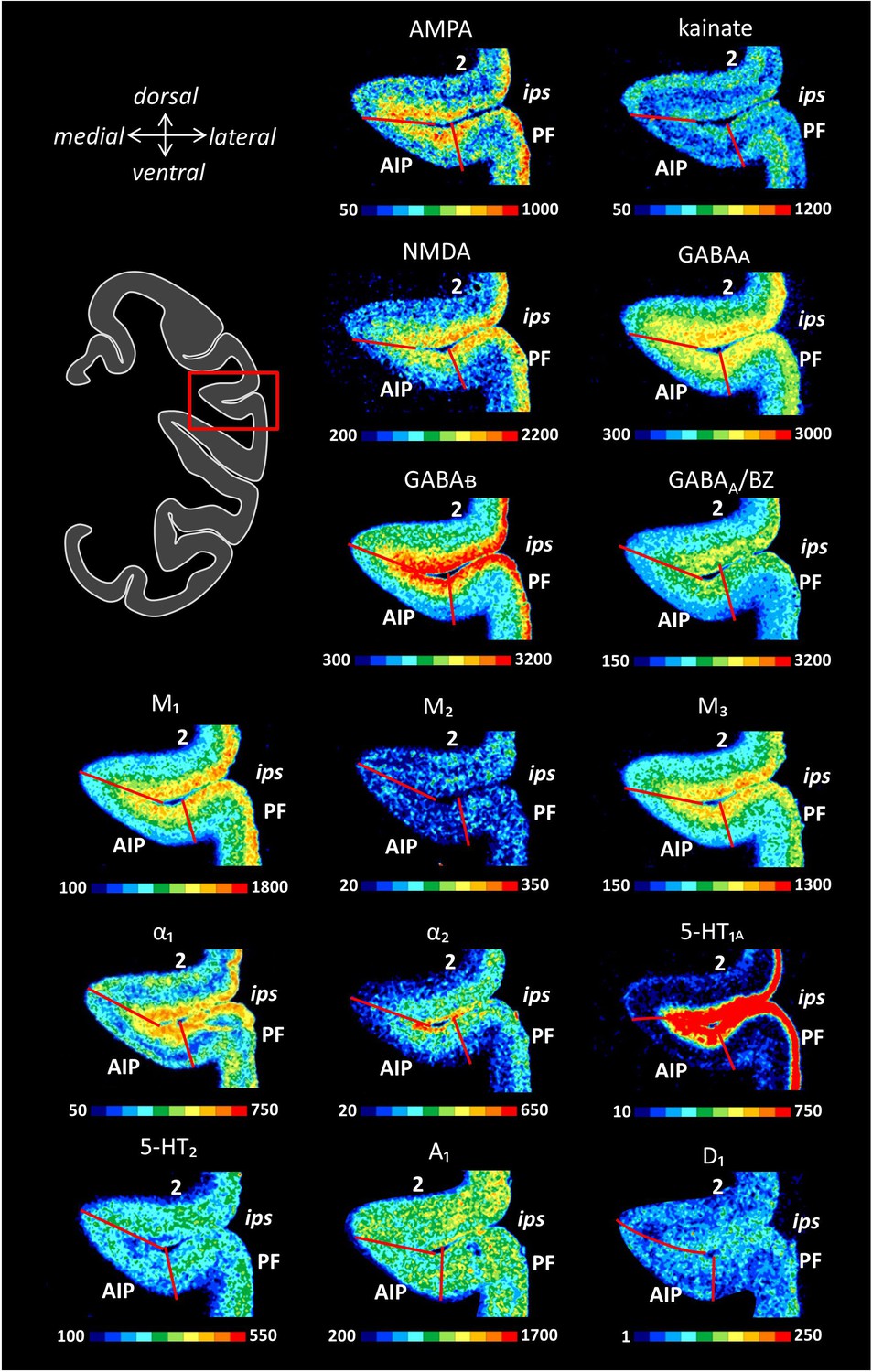
Receptor distribution patterns in the rostral portion of the IPS.
Receptor distribution patterns in area AIP illustrated for the 15 receptors studied. For further details, see Figure 10—figure supplement 1.
Figure 11 with 1 supplement
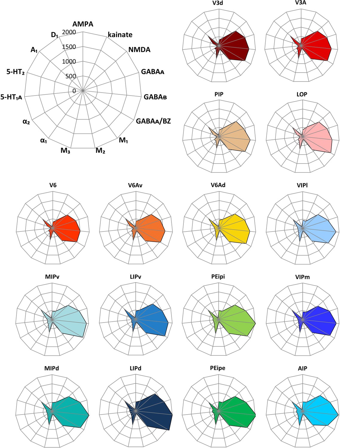
Receptor fingerprints of the examined brain areas.
Absolute densities in fmol/mg protein of 15 receptors are displayed in polar coordinate plots (scaling 0–2000 fmol/mg protein). For aesthetical reasons, the standard deviations are not displayed in the fingerprints. For mean (and s.d.) densities of each area and receptor type see Table 1. The positions of the different receptor types and the axis scaling are identical in all polar plots, and specified in the polar plot at the top left corner of the figure. For abbreviations, see Figure 2.
Figure 11—figure supplement 1
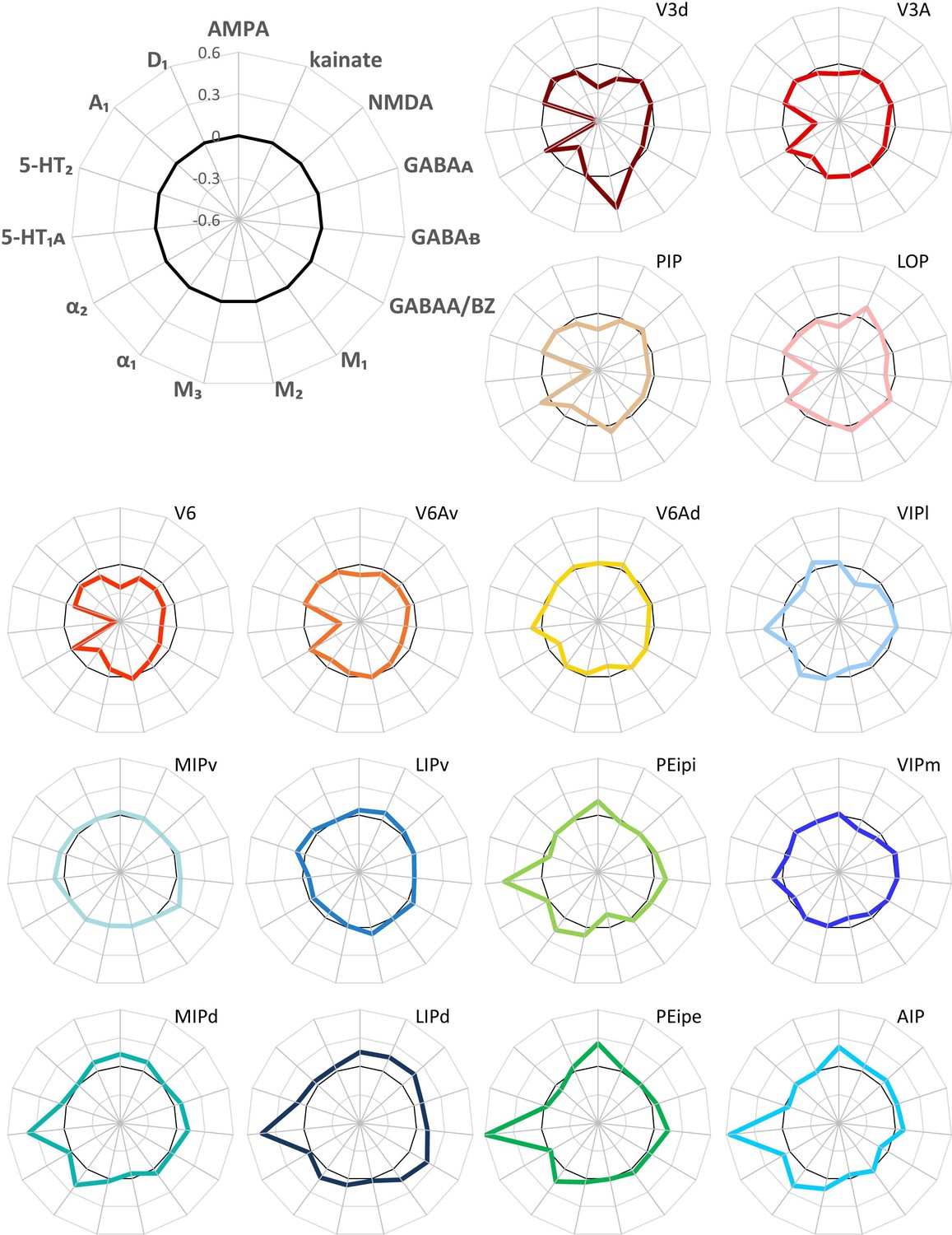
Normalized receptor fingerprints of the examined brain areas.
Polar plots (scaling −0.6/+0.6) showing the normalized receptor concentration of all 15 receptors. Normalization of the receptor concentrations was calculated based on each receptor’s mean over all IPS areas. Black thick line indicates the position where the receptor concentration was equal to the mean receptor concentration averaged over all IPS areas.
Figure 12
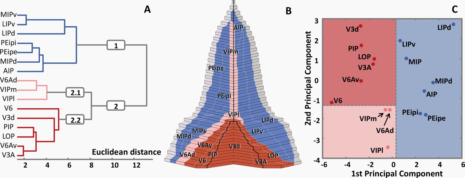
Receptor-driven clustering of the IPS subdivisions.
(A) Hierarchical cluster analysis reveals 3 receptor-architectonically distinct clusters: a caudal cluster with visual areas (blue); an intermediate group of areas VIPm, VIPl and V6Ad (pink); and a rostral group consisting of all areas located on the bilateral walls of IPS (red). (B) Three clusters are displayed in the 2D flat map, same color coding as in (A). (C) Principal component analysis. The distances between areas represent the Eigenvalues of the first and second principal components, three clusters are clearly segregated by the first and second principal component, same color coding as in (A) and (B). For abbreviations, see Figure 2.
Figure 13
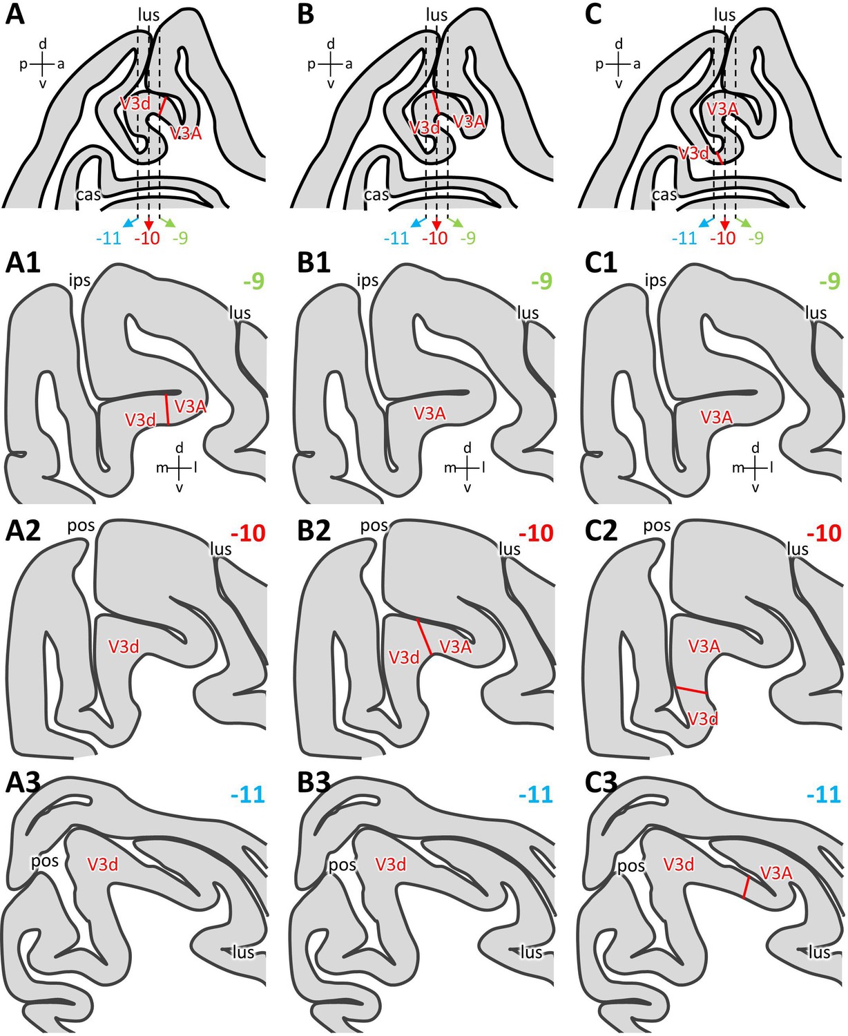
Inter-individual variability in the position of the V3d/V3A border.
Schematic representation of an exemplary parasagittal section located 10 mm to the right of the midline, on which variations in the position of the V3d/V3A border in relation to the anectant gyrus are illustrated (A, B, C). Dashed lines indicate the rostro-caudal position of the coronal sections shown below and which are located 9 mm (A1, B1, C1), 10 mm (A2, B2, C2) and 11 mm (A3, B3, C3) caudal to the interaural surface (Saleem and Logothetis, 2012). (A1–A3) Schematic representation of areas found on the anectant gyrus when the V3d/V3A border was detected on its rostral wall (A). (B1–B3) Schematic representation of areas found on the anectant gyrus when the V3d/V3A border was detected on its apex (B). (C1–C3) Schematic representation of areas found on the anectant gyrus when the V3d/V3A border was detected on its caudal wall (C). Abbreviations: a anterior, cas calcarine sulcus, d dorsal, ips intraparietal sulcus, l lateral, lus lunate sulcus, m medial, p posterior, pos parieto-occipital sulcus, v ventral.
Tables
Table 1
Mean receptor densities of IPS areas in fmol/mg protein.
| AMPA | Kainate | NMDA | GABAA | GABAB | GABAA/BZ | M₁ | M₂ | M₃ | α₁ | α₂ | 5-HT₁A | 5-HT₂ | A₁ | D₁ | ||
|---|---|---|---|---|---|---|---|---|---|---|---|---|---|---|---|---|
| AIP | mean | 506.5 | 541.0 | 1284.4 | 1564.8 | 1958.2 | 1565.2 | 924.0 | 128.2 | 819.3 | 409.3 | 306.0 | 348.6 | 319.4 | 800.7 | 77.3 |
| s.d. | 70.1 | 101.0 | 124.5 | 238.1 | 277.9 | 226.9 | 154.5 | 39.3 | 91.8 | 46.0 | 53.3 | 35.2 | 75.9 | 180.4 | 5.1 | |
| LIPd | mean | 485.5 | 592.5 | 1397.0 | 1621.0 | 2012.4 | 2097.2 | 1028.2 | 136.7 | 788.6 | 374.2 | 291.7 | 323.3 | 364.9 | 832.3 | 82.0 |
| s.d. | 67.4 | 60.7 | 199.1 | 159.6 | 290.6 | 350.5 | 186.6 | 41.2 | 113.8 | 28.3 | 25.6 | 50.1 | 73.2 | 183.2 | 7.3 | |
| LIPv | mean | 443.2 | 551.0 | 1241.1 | 1508.9 | 1783.3 | 1832.0 | 912.2 | 143.3 | 722.4 | 310.6 | 271.9 | 209.0 | 361.8 | 834.4 | 77.6 |
| s.d. | 64.8 | 34.3 | 189.3 | 160.3 | 250.3 | 167.5 | 135.7 | 38.0 | 100.9 | 25.5 | 23.7 | 22.2 | 62.8 | 127.6 | 6.4 | |
| PEipe | mean | 522.3 | 526.7 | 1203.0 | 1570.2 | 2064.6 | 1792.6 | 943.6 | 134.2 | 766.0 | 390.0 | 278.6 | 355.6 | 323.5 | 733.6 | 81.6 |
| s.d. | 53.4 | 96.6 | 236.5 | 226.5 | 269.9 | 164.1 | 111.0 | 49.6 | 80.1 | 36.8 | 53.0 | 55.9 | 76.8 | 152.8 | 8.8 | |
| PEipi | mean | 483.4 | 495.8 | 1190.1 | 1549.1 | 2024.8 | 1802.3 | 933.4 | 114.6 | 800.2 | 389.2 | 288.0 | 312.3 | 311.2 | 789.8 | 79.2 |
| s.d. | 85.4 | 95.7 | 135.4 | 194.4 | 286.9 | 114.8 | 77.5 | 40.6 | 108.3 | 39.4 | 53.5 | 50.5 | 55.8 | 111.2 | 7.1 | |
| MIPv | mean | 435.0 | 517.2 | 1173.8 | 1549.0 | 1875.7 | 1927.6 | 903.8 | 132.0 | 723.2 | 342.9 | 288.0 | 245.8 | 356.0 | 826.9 | 79.1 |
| s.d. | 72.9 | 62.9 | 217.1 | 175.1 | 263.9 | 162.7 | 93.7 | 34.9 | 97.2 | 33.7 | 44.9 | 62.6 | 51.8 | 131.0 | 6.7 | |
| MIPd | mean | 475.7 | 562.3 | 1210.8 | 1598.3 | 2020.1 | 1779.9 | 951.8 | 126.4 | 760.7 | 406.0 | 291.5 | 307.0 | 350.0 | 796.5 | 85.8 |
| s.d. | 70.9 | 84.8 | 186.9 | 171.9 | 321.2 | 93.0 | 102.7 | 36.5 | 81.7 | 39.1 | 47.7 | 82.2 | 66.4 | 154.9 | 6.7 | |
| VIPl | mean | 431.8 | 423.2 | 1130.1 | 1445.1 | 1829.8 | 1606.6 | 858.7 | 121.6 | 753.2 | 368.3 | 272.5 | 264.3 | 317.7 | 718.4 | 84.3 |
| s.d. | 75.4 | 91.4 | 151.7 | 243.6 | 203.3 | 142.8 | 81.0 | 41.3 | 76.7 | 27.3 | 49.9 | 28.7 | 69.8 | 120.8 | 9.5 | |
| VIPm | mean | 426.7 | 453.9 | 1104.5 | 1534.2 | 1847.5 | 1714.7 | 856.7 | 119.9 | 725.3 | 338.2 | 270.2 | 244.6 | 321.1 | 806.6 | 76.3 |
| s.d. | 69.3 | 90.1 | 212.8 | 180.7 | 346.4 | 78.8 | 83.7 | 41.3 | 99.9 | 49.7 | 48.5 | 34.3 | 59.0 | 148.1 | 9.1 | |
| PIP | mean | 348.6 | 494.9 | 1241.2 | 1400.7 | 1702.0 | 1629.8 | 857.7 | 142.5 | 666.3 | 292.3 | 310.5 | 110.6 | 336.4 | 795.1 | 73.3 |
| s.d. | 58.7 | 61.3 | 119.2 | 162.5 | 303.9 | 125.5 | 134.0 | 42.3 | 104.3 | 64.7 | 27.0 | 54.6 | 74.8 | 136.8 | 8.3 | |
| LOP | mean | 361.6 | 573.1 | 1190.1 | 1396.3 | 1614.2 | 1774.2 | 885.3 | 140.4 | 707.3 | 317.0 | 296.3 | 143.2 | 336.1 | 758.4 | 75.5 |
| s.d. | 59.0 | 69.3 | 146.2 | 157.7 | 224.2 | 175.3 | 65.5 | 33.3 | 100.3 | 47.6 | 25.1 | 57.1 | 67.3 | 135.1 | 6.0 | |
| V3A | mean | 378.0 | 492.2 | 1189.0 | 1455.3 | 1652.9 | 1647.1 | 878.7 | 133.2 | 742.1 | 293.6 | 292.1 | 144.9 | 332.7 | 810.6 | 74.1 |
| s.d. | 78.5 | 69.4 | 120.1 | 294.1 | 280.1 | 51.5 | 125.0 | 25.4 | 100.9 | 62.0 | 50.2 | 50.3 | 71.0 | 236.9 | 11.9 | |
| V3d | mean | 317.9 | 452.0 | 1213.6 | 1476.8 | 1644.7 | 1627.7 | 906.6 | 178.9 | 727.6 | 249.6 | 294.6 | 87.9 | 331.0 | 827.0 | 74.9 |
| s.d. | 66.2 | 82.4 | 129.3 | 405.2 | 289.8 | 120.2 | 99.0 | 60.5 | 93.5 | 45.8 | 37.8 | 37.3 | 74.0 | 192.6 | 7.0 | |
| V6Ad | mean | 427.2 | 536.3 | 1148.7 | 1450.0 | 1679.1 | 1698.1 | 904.3 | 118.3 | 710.1 | 329.1 | 248.6 | 245.9 | 323.2 | 782.7 | 80.4 |
| s.d. | 71.1 | 87.4 | 116.5 | 265.0 | 335.4 | 141.4 | 74.3 | 36.7 | 92.9 | 35.5 | 36.0 | 46.3 | 68.8 | 147.4 | 8.1 | |
| V6Av | mean | 373.8 | 483.1 | 1115.6 | 1393.7 | 1595.7 | 1543.9 | 857.0 | 134.3 | 706.8 | 305.4 | 286.3 | 136.9 | 336.9 | 790.1 | 76.0 |
| s.d. | 71.3 | 59.5 | 71.1 | 193.3 | 277.0 | 116.1 | 64.7 | 32.7 | 91.5 | 29.3 | 23.2 | 38.7 | 52.5 | 106.2 | 4.6 | |
| V6 | mean | 319.2 | 457.8 | 1073.0 | 1317.3 | 1505.0 | 1514.6 | 832.1 | 136.7 | 675.9 | 260.1 | 274.9 | 99.8 | 301.8 | 754.1 | 71.5 |
| s.d. | 57.7 | 58.9 | 142.3 | 233.8 | 397.6 | 34.2 | 66.2 | 40.6 | 117.0 | 47.5 | 37.1 | 39.4 | 73.5 | 129.2 | 6.7 |
Table 2
Incubation protocols.
| Transmitter | Receptor | Ligand (nM) | Property | Displacer | Incubation buffer | Pre-incubation | Main incubation | Final rinsing |
|---|---|---|---|---|---|---|---|---|
| Glutamate | AMPA | [3H]-AMPA (10.0) | Ag | Quisqualate (10 μM) | 50 mM Tris-acetate (pH 7.2) [+ 100 mM KSCN]* | 3x10 min, 4°C | 45 min, 4°C | 1) 4x4 sec2) Acetone/glutaraldehyde(100 ml + 2,5 ml), 2x2 sec, 4°C |
| NMDA | [3H]-MK-801 (3.3) | Ant | (+)MK-801 (100 μM) | 50 mM Tris-acetate (pH 7.2) + 50 μM glutmate [+ 30 μM glycine + 50 μM spermidine]* | 15 min, 4°C | 60 min, 22°C | 1) 2x5 min, 4°C2) Distilled water, 1x22°C | |
| Kainate | [3H]-Kainate (9.4) | Ag | SYM 2081 (100 μM) | 50 mM Tris-acetate (pH 7.2) [+ 10 mM Ca2+-acetate]* | 3x10 min, 4°C | 45 min, 4°C | 1) 3x4 sec2) Acetone/glutaraldehyde(100 ml + 2,5 ml), 2x2 sec, 22°C | |
| GABA | GABAA | [3H]-Muscimol (7.7) | Ag | GABA (10 μM) | 50 mM Tris-citrate (pH 7.0) | 3x5 min, 4°C | 40 min, 4°C | 1) 3x3 sec, 4°C2) Distilled water, 1x22°C |
| GABAB | [3H]-CGP 54626 (2.0) | Ant | CGP 55845 (100 μM) | 50 mM Tris-HCl (pH 7.2) + 2.5 mM CaCl2 | 3x5 min, 4°C | 60 min, 4°C | 1) 3x2 sec, 4°C2) Distilled water, 1x22°C | |
| GABAA/BZ | [3H]-Flumazenil (1.0) | Ant | Clonazepam (2 μM) | 170 mM Tris-HCl (pH 7.4) | 15 min, 4°C | 60 min, 4°C | 1) 2x1 min, 4°C2) Distilled water, 1x22°C | |
| Acetylcholine | M1 | [3H]-Pirenzepine (1.0) | Ant | Pirenzepine (2 μM) | Modified Krebs buffer (pH 7.4) | 15 min, 4°C | 60 min, 4°C | 1) 2x1 min, 4°C2) Distilled water, 1x22°C |
| M2 | [3H]-Oxotremorine-M (1.7) | Ag | Carbachol (10 μM) | 20 mM HEPES-Tris (pH 7.5) + 10 mM MgCl2 + 300 nM Pirenzepine | 20 min, 22°C | 60 min, 22°C | 1) 2x2 min, 4°C2) Distilled water, 1x22°C | |
| M3 | [3H]-4-DAMP (1.0) | Ant | Atropine sulfate (10 μM) | 50 mM Tris-HCl (pH 7.4) + 0.1 mM PSMF + 1mM EDTA | 15 min, 22° C | 45 min, 22° C | 1) 2x5 min, 4° C2) distilled water, 1x22°C | |
| Noradrenaline | α1 | [3H]-Prazosin (0.2) | Ant | Phentolamine Mesylate (10 μM) | 50 mM Na/K-phosphate buffer (pH 7.4) | 15 min, 22°C | 60 min, 22°C | 1) 2x5 min, 4°C2) Distilled water, 1x22°C |
| α2 | [3H]-UK 14,304 (0,64) | Ag | Phentolamine Mesylate (10 μM) | 50 mM Tris-HCl + 100 μM MnCl2 (pH 7.7) | 15 min, 22°C | 90 min, 22°C | 1) 5 min, 4°C2) Distilled water, 1x22°C | |
| Serotonin | 5-HT1A | [3H]-8-OH-DPAT (1.0) | Ag | 5-Hydroxy-tryptamine (1 μM) | 170 mM Tris-HCl (pH 7.4) [+ 4 mM CaCl2 + 0.01% ascorbate]* | 30 min, 22°C | 60 min, 22°C | 1) 5 min, 4°C2) Distilled water, 3x22°C |
| 5-HT2 | [3H]-Ketanserin (1.14) | Ant | Mianserin (10 μM) | 170 mM Tris-HCl (pH 7.7) | 30 min, 22°C | 120 min, 22°C | 1) 2x10 min, 4°C2) Distilled water, 3x22°C | |
| Dopamine | D1 | [3H]-SCH 23390 (1.67) | Ant | SKF 83566 (1 μM) | 50 mM Tris-HCl + 120 mM NaCl + 5 mM KCl + 2 mM CaCl2 + 1 mM MgCl2 (pH 7.4) | 20 min, 22°C | 90 min, 22°C | 1) 2x20 min, 4°C2) Distilled water, 1x22°C |
| Adenosine | A1 | [3H]-DPCPX (1.0) | Ant | R-PIA (100 μM) | 170 mM Tris-HCl + 2 Units/I Adenosine deaminase [+ 100 μM Gpp(NH)p]* (pH 7.4) | 15 min, 4°C | 120 min, 22°C | 1) 2x5 min, 4°C2) Distilled water, 1x22°C |
-
* Only included in the main incubation. Ag agonist, Ant antagonist
Additional files
Download links
A two-part list of links to download the article, or parts of the article, in various formats.
Downloads (link to download the article as PDF)
Open citations (links to open the citations from this article in various online reference manager services)
Cite this article (links to download the citations from this article in formats compatible with various reference manager tools)
Receptor-driven, multimodal mapping of cortical areas in the macaque monkey intraparietal sulcus
eLife 9:e55979.
https://doi.org/10.7554/eLife.55979


