Combining agent-based, trait-based and demographic approaches to model coral-community dynamics
Figures
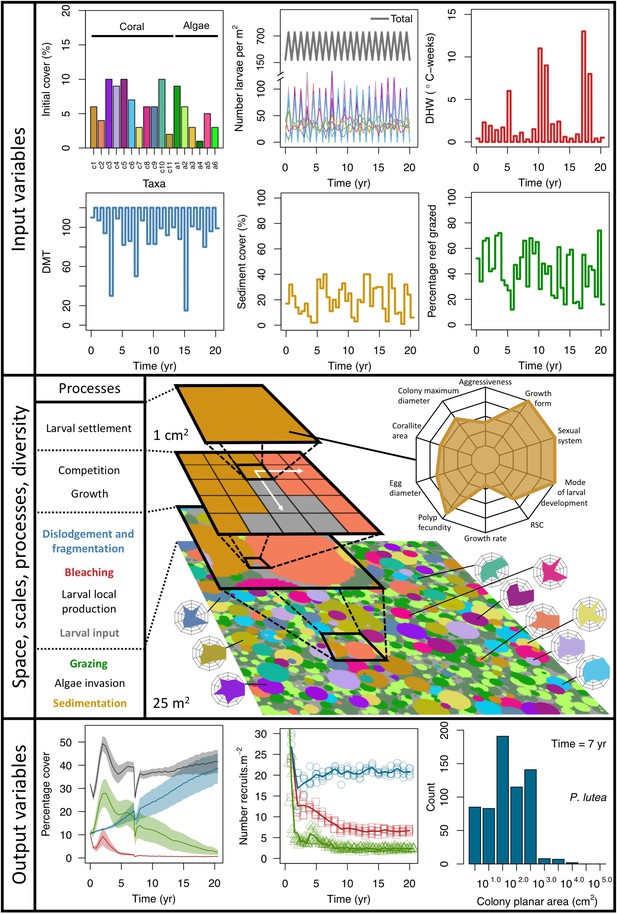
Description of the agent-based model.
Six different variables as model inputs determine (i) initial community composition, (ii) number of larvae coming from the regional pool (total number divided among different species, with annual supply for spawning species, and biannual supply for brooding species), (iii) thermal stress in degree-heating weeks, (iv) hydrodynamic regime intensity expressed as dislodgment mechanical threshold (unitless), (v) sedimentation, and (vi) the percentage of reef grazed. All variables are inputs at every time period except for the initial community composition that is determined during initialization. The model represents a 25 m2 coral reef community and is composed of 1 cm2 cell agents. Once every time step, living agents (algae and corals) grow by converting their neighbouring agents within a certain radius (white arrows in middle panel). Different processes affect the community at different spatial scales. For instance, the grazing process lasts until the imposed percentage cover grazed over the entire reef is reached. In contrast, coral colonies are individually considered for dislodgment during hydrodynamic disturbance and a single agent is potentially converted into a new coral recruit when larvae settle successfully. Radar charts represent the functional characteristics of coral species (defined by a specific colour): each vertex corresponds to a functional trait and the coloured polygon indicates the trait values of the species (higher values are farther away from the centre of the web). At the end of each time step, the model provides the percentage cover, the number of coral recruits, and the size of each colony for every taxon, and optionally, the reef rugosity created by coral colonies (bottom panel). The benthic community at the largest scale is a screenshot of the model output.

Ordering of processes in the coral agent-based model: white rectangles represent processes, dark grey rectangles with white text are input data, and light grey rectangles with black text are outputs.
Large white arrows define the ordering of processes and black arrows show the direction of data transfer; dashed black arrows are optional processes (not activated for the analyses we present here). The order of occurrence of coral reproduction, bleaching, and colony dislodgement and fragmentation is imposed to simulate recruitment failure due to the occurrence of a disturbance prior to reproduction. The intensity of waves and cyclones is expressed as a dimensionless dislodgment mechanical threshold; thermal stress is expressed in degree-heating weeks.
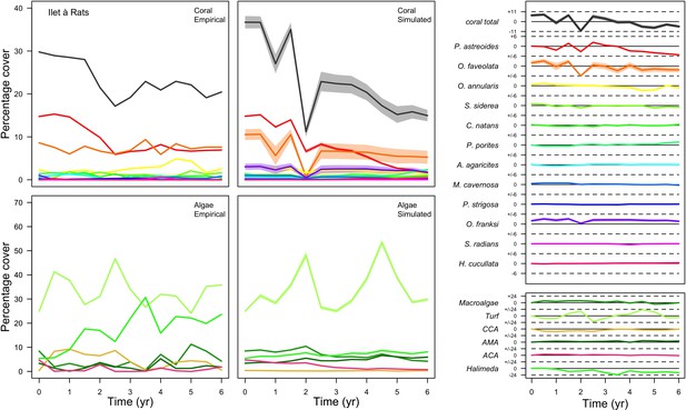
Comparison of empirical and simulated taxa cover for the combination of parameter values providing the best fit for site Ilet à Rats.
Solid lines in the simulated time series are the percentage cover means (averaged over five replicates) and the shaded areas show the standard error. The right panels display the cover difference between simulated and empirical time series.
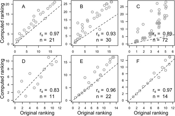
Correlation analyses between the original aggressiveness rankings and the selected global computed ranking for each study.
(A: Sheppard, 1979; B: Abelson and Loya, 1999; C: Dai, 1990; D: Connell et al., 2004; E: Lang, 1973; F: Logan, 1984). Also displayed are the Spearman ρ (rs), the number of species (n) and the identity line (dashed lines) for visual aid. All p<0.001 except for D, where p=0.003.
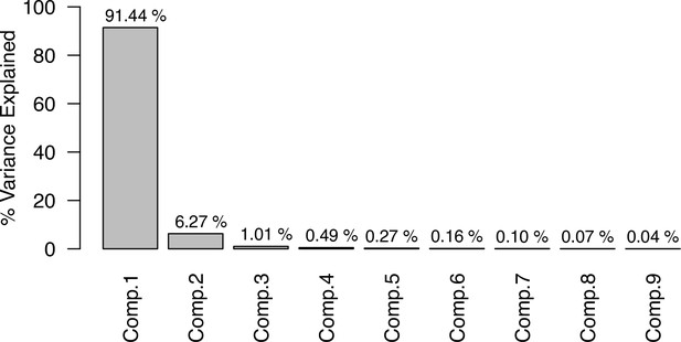
Percentage of variance explained by the nine first eigenvectors produced by the PCA on the averaged phylogenetic distance matrix.
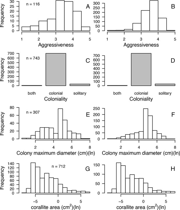
Comparisons of frequency distributions of trait values between the original dataset (left column) and the imputed dataset (right column) for aggressiveness (A, B); coloniality (C, D); colony maximum diameter (E, F); corallite area (G, H) (total n = 798).
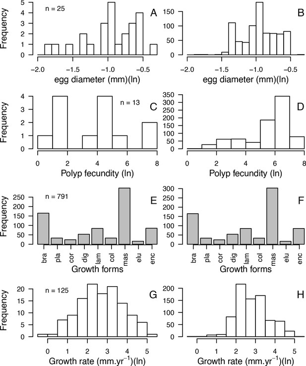
Comparisons of frequency distributions of trait values between the original dataset (left column) and the imputed dataset (right column) for egg diameter (A, B); polyp fecundity (C, D); growth forms: branching (bra), plate (pla), corymbose (cor), digitate (dig), laminar (lam), columnar (col), massive (mas), encrusting long upright (elu), encrusting (enc) (E, F); growth rate (G, H) (total n = 798).
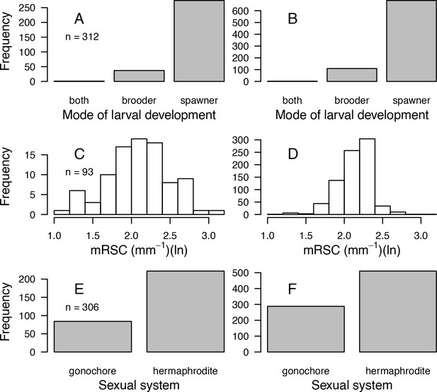
Comparisons of frequency distributions of trait values between the original dataset (left column) and the imputed dataset (right column) for model of larval development (A, B); microscopic reduced scattering coefficient (mRSC; C, D); sexual system (E, F) (total n = 798).
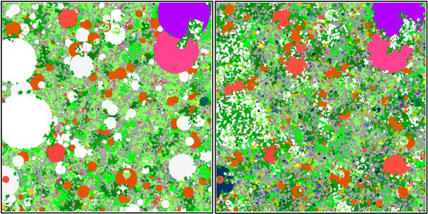
Screenshots displaying a 25 m2 of the benthic community at Ilet à Rats taken after the execution of the bleaching process (left) and at the end of the same 6-month time step (right).
We used parameter values calibrated with the empirical data describing this specific site (see Appendix 3). Coral colonies (pink, orange, blue, dark blue, white and light grey shapes) and algae (macroalgae, turf, allopathic macroalgae, and crustose coralline algae are in green, light green, dark green and beige shapes, respectively) compete spatially. Colourful coral colonies were not affected by the thermal disturbance, light grey colonies bleached and survived, and white colonies died. Grey and yellow agents represent barren ground and sand, respectively.
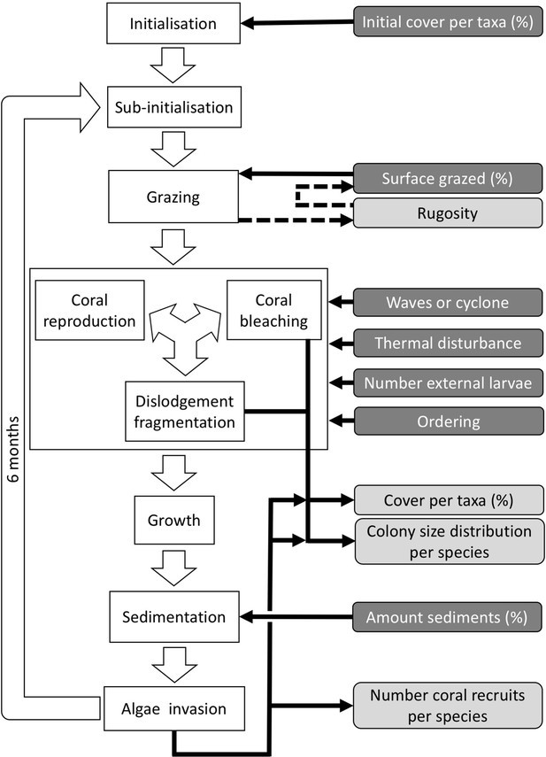
Ordering of the most important processes in the coral agent-based model: white rectangles represent processes, dark grey rectangles with white text are input data, and light grey rectangles with black text are outputs.
Large white arrows define the ordering of processes and black arrows show the direction of data transfer; dashed black arrows are optional processes. The order of occurrence of coral reproduction, bleaching, and colony dislodgement and fragmentation is imposed to simulate recruitment failure due to the occurrence of a disturbance prior to reproduction. The intensity of waves and cyclones is expressed as a dimensionless dislodgment mechanical threshold; thermal stress is expressed in degree-heating weeks.
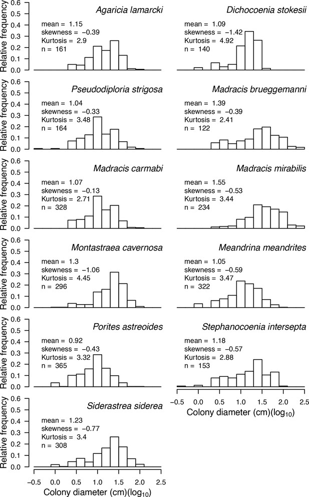
Size-class distributions of 11 Caribbean coral species (data collected in Curaçao in 1996, E. H. Meesters and R. P. M. Bak, personal communication, May 2017).
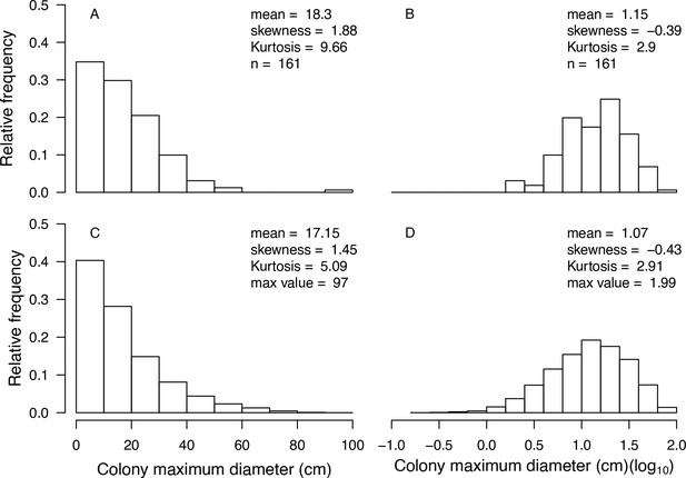
Example of a visual comparison of colony size distributions between the real data (A, B) and the one obtained with the command nextSkewDistFun (C, D) for Agaricia lamarcki (n = 10,000).
Real data were collected in Curaçao in 1996 (E. H. Meesters and R. P. M. Bak, personal communication, May 2017). We obtained the simulated distributions with bias = −1.9 and skew = 0.88.
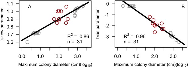
Linear regression models for skew (A) and bias (B) expressed as a function of maximum colony diameter.
Red circles are values of skew and bias manually obtained by comparison with empirical colony size class distributions (E. H. Meesters and R. P. M. Bak, personal communication, May 2017). Grey circles are the values of skew and bias we defined for the 20 species we added in order to increase the sample size and range of colony sizes. Also displayed are the least squares linear regression and the corresponding coefficient of determination.
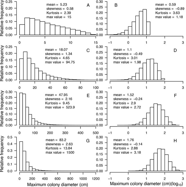
Examples of modeled species-specific colony diameter distributions (n = 100,000).
From top to bottom: Acropora nana (A, B), Acanthastrea echinata (C, D), Acropora longitcyathus (E, F), Acropora florida (G, H). Max value = maximum colony diameter.
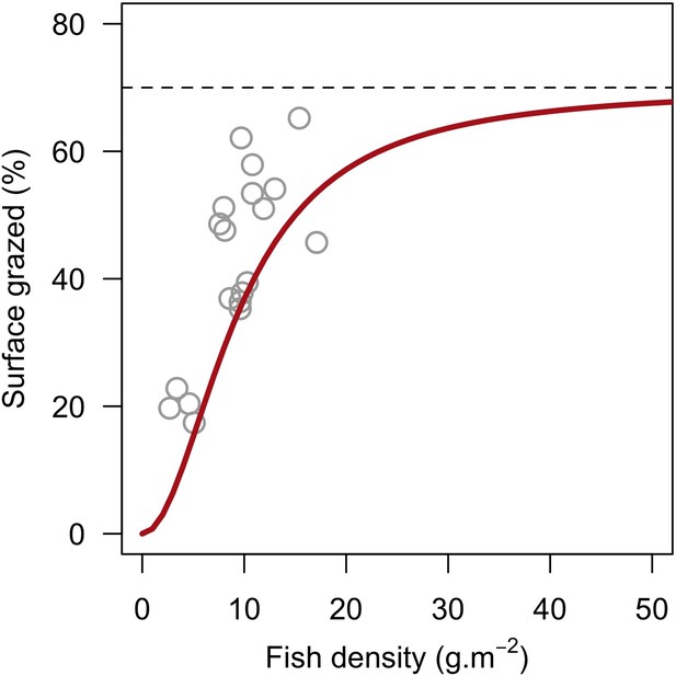
Model defining the percentage of reef surface grazed as a function of herbivorous fish density.
Grey circles are averaged surface of reefs maintained in a cropped state as a function of pooled Acanthuridae spp. and Scaridae spp. densities in 19 Caribbean reefs (Williams and Polunin, 2001). The red line is the asymptotic model we defined: y = 70x2 / (90 + x2).
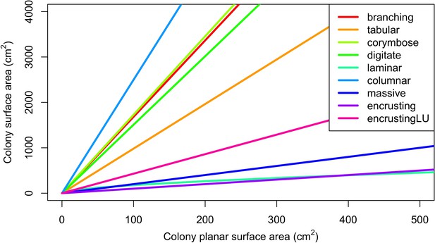
Conversion of colony planar area into three-dimensional surface area using geometric models for each growth form (McWilliam et al., 2018a).
The conversion necessitated considering the planar surface area of each colony as circular.
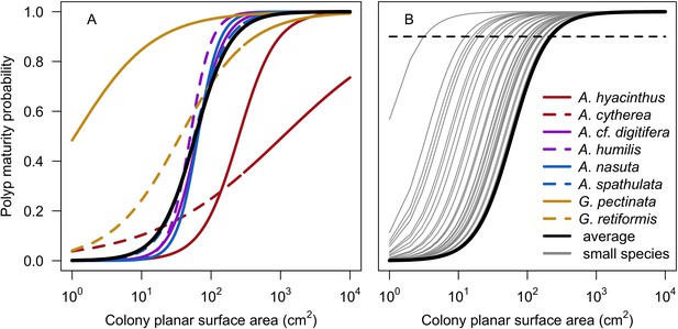
Probability of a polyp to be mature depending on the size of the colony.
Coloured lines (i.e. red, purple and yellow) in panel A displays the eight species-specific models established by Álvarez-Noriega et al. (2016); the black line in panels A and B represents the model obtained by averaging coefficient over the eight species. Panel B displays the 50 models we defined for the species reaching a maximum planar surface area inferior to 218.9 cm2. The horizontal dashed line indicates 0.9 probability; it intercepts with individual grey lines when the colony of the corresponding species reaches its maximum planar area (assuming the latter is circular).
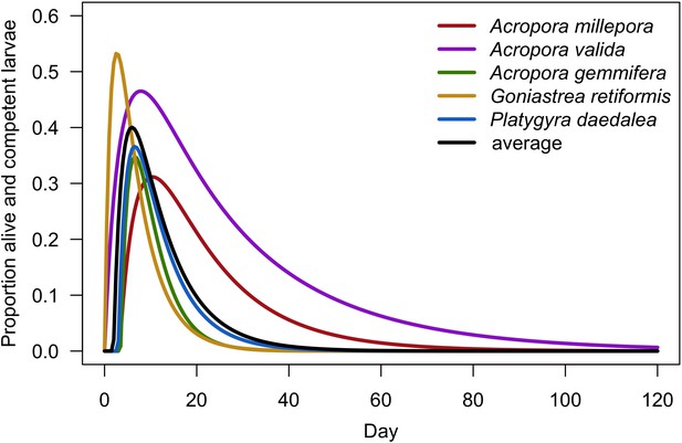
Prediction of the dispersal potential depending on time for five coral species (Connolly and Baird, 2010).
The black line represents the prediction from the average model (i.e. we averaged the coefficients of the five species-specific models).
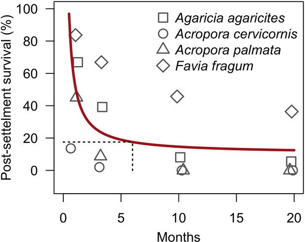
Proportion of larvae surviving after settlement as a function of time (from Figure 8b in Ritson-Williams et al., 2016).
Twelve and 20 replicate tiles (covered with the CCA Hydrolithon boergesenii) were used for brooding (A. agaricites, Favia fragum) and spawning species (A. cervicornins, A. palamata), respectively. Each tile received initially three recruits of a same species. The grey symbols represent the mean percentage of surviving recruits by tile. The red line is the least-squares regression model we established, considering each point as a single observation (Appendix 2—table 13). The black dashed lines show the proportion of recruits at six months after settlement (plxs = 0.18). Points have been offset slightly to improve visibility.
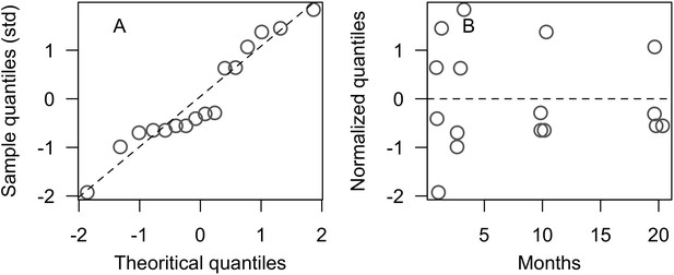
Residual diagnostic plots of the coral recruitment model we established based on Ritson-Williams et al. (2016)’s results (Appendix 2—figure 11): normal quantile plot (A) and residual plot (B) respectively show that the standardized residuals are normally and homogeneously distributed.
Points in B have been offset slightly to improve visibility.
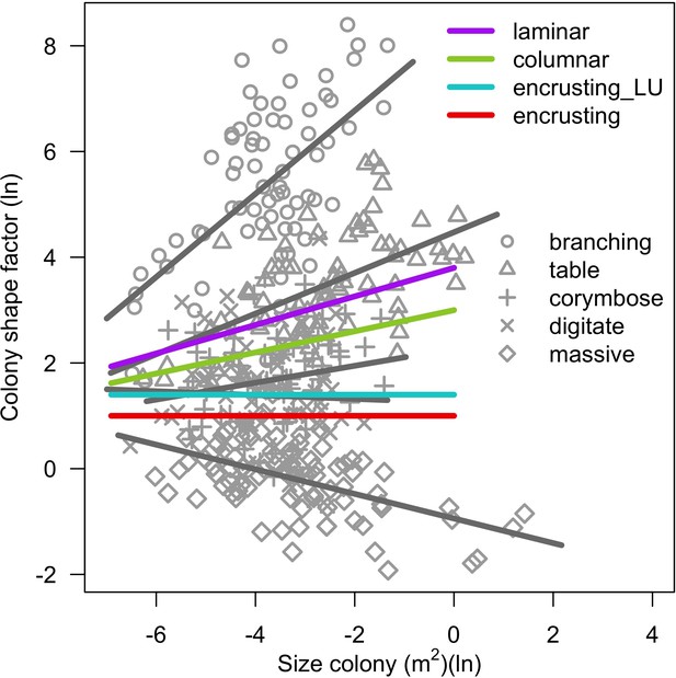
Colony shape factor as a function of colony planar area for different colony growth forms.
Grey symbols represent a single colony and lines are fitted least-squares regression lines per growth forms (Madin et al., 2014). The colored lines represents the model we implemented in the coral ABM for the growth forms not considered in Madin et al. (2014) (see text; Appendix 2—table 14).
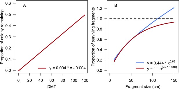
Models predicting the proportion of a branching colony remaining and potentially surviving as a function of dislodgement mechanical threshold (DMT, A) and the proportion of surviving fragments as a function of their length (B).
The blue line in panel B corresponds to the empirical relationship established by Highsmith et al. (1980), the red line is the model we defined.
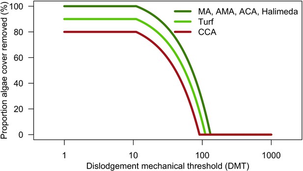
Proportions of algae removed from the reef depending on cyclone intensity (DMT) (Appendix 2—table 15).
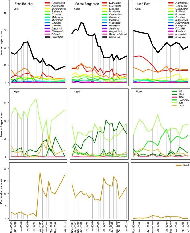
Composition of the benthic communities in the three Caribbean sites.
Vertical grey bars indicate the dates at which data were collected. The data were collected by the Observatoir du Milieu Marin Martiniquais for the program Initiative Française pour les REcifs COralliens.
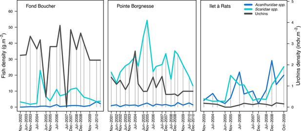
Population densities of herbivore fish and sea urchins (Diadema antillarum and Echinometra viridis combined) measured in the three Caribbean sites.
Vertical grey bars indicate the dates at which data were collected. The data were collected by the Observatoir du Milieu Marin Martiniquais for the program Initiative Française pour les REcifs COralliens.
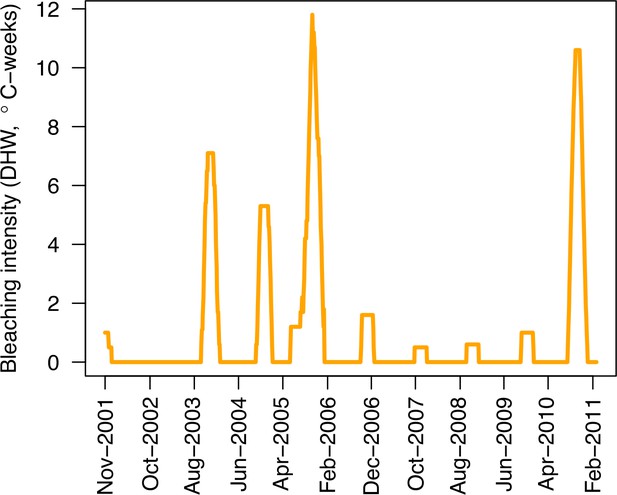
Evolution of the thermal stress in degree heating weeks affecting the three Caribbean sites (US National Oceanic and Atmospheric Administration’s data server ERDDAP).
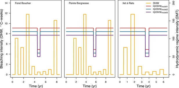
Values of thermal stress (in degree heating weeks) and hydrodynamic thresholds (dislodgment mechanical threshold) imposed in the model at each time step for the three Caribbean sites.
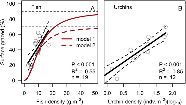
Models defining the percentage of reef surface grazed as a function of herbivore density.
Fish densities were measured in 19 Caribbean reefs (A, Williams and Polunin, 2001). Also shown are the surface grazed averaged by site (grey circles), the significant least-squares regression line (black solid line; equation: Y = 15.5 + 2.9X) and the two asymptotic models we defined for modeling fish grazing pressure at higher fish densities (i.e. densities not observed in the study). Sea urchin densities were measured in a cage exclusion field experiment (B, Sammarco, 1980). Grey circles are surface grazed averaged by site, black lines are least-squares regressions (black solid line; equation: Y = 8.9 + 29.5X). Dashed lines represent the 95% confidence bands.
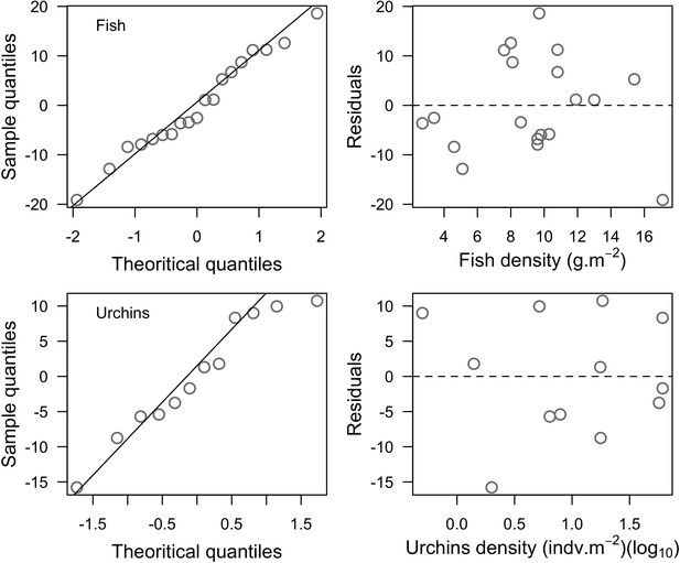
Normal quantile plots (left column) and residual plots (right column) respectively verifying the assumptions of normality and equal variance distribution of the residuals of the least-squares linear regression models established to model fish (top row) and urchin grazing pressure (bottom row).
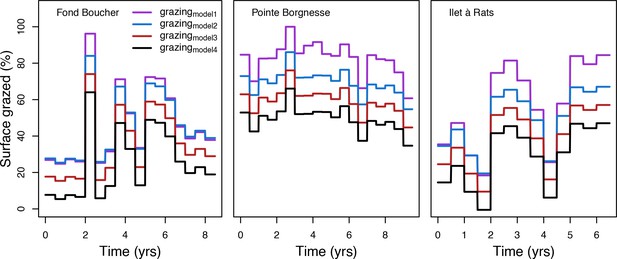
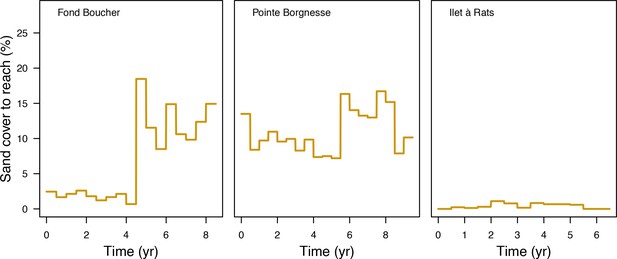
Percentage cover grazed imposed in the model at each time step for the three Caribbean sites.
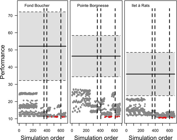
Evolution of the performance (smaller values show better performance) as a function of the order at which runs were launched for the three Caribbean sites (n = 672, 680 and 669 for Fond Boucher, Pointe Borgnesse and Ilet à Rats, respectively).
Each grey dot represents the performance of a given parameter combination (averaged over five replicates). The 20 parameter points showing the best performance are shown in red. The vertical dashed lines separate the simulations launched respectively in round one, two, three and four. The horizontal black lines and grey areas show the mean and 95% confidence intervals of the null distributions of performance values (n = 1000).
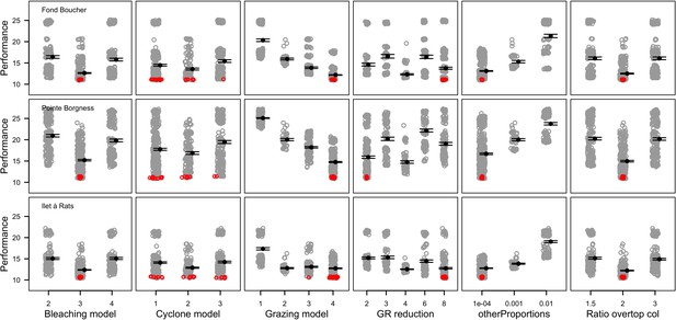
Performance comparison of all the combinations of parameter values simulated for six of the 12 parameters calibrated (n = 672, 680 and 669 for Fond Boucher, Pointe Borgnesse and Ilet à Rats, respectively).
Grey circles represent the performance of a unique parameter combination (averaged over five replicates). Smaller values show better performance. Black dots and error bars show the mean ± standard error by parameter value. Red circles show the 20 parameter combinations providing the best performance.
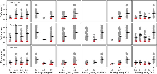
Performance comparison of all the combinations of parameter values simulated for six of the 12 parameters calibrated (n = 672, 680 and 669 for Fond Boucher, Pointe Borgnesse and Ilet à Rats, respectively).
Grey circles represent the performance of a unique parameter combination (averaged over five replicates). Smaller values show better performance. Black dots and errors bars show the mean ± standard error by parameter value. Red circles show the 20 parameter combinations providing the best performance.
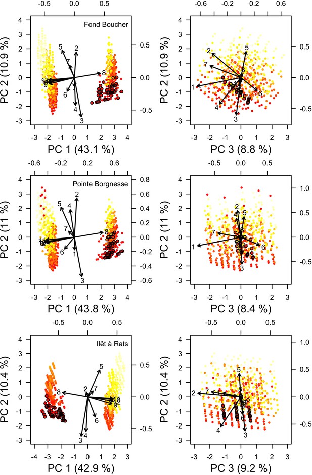
Projection in the parameter space of the combinations of parameter values selected during the calibration for each site (n = 672, 680 and 669 for Fond Boucher, Pointe Borgnesse and Ilet à Rats, respectively).
Arrows indicate parameter loading; numbers designate parameters (coordinates values are displayed on the top and right sides): (1) bleaching model; (2) cyclone model; (3) grazing model; (4) growth rate reduction; (5) otherProportions; (6) prob cover crustose coralline algae; (7) ratio overtop colony; (8) prob grazing macroalgae; (9) prob grazing allopathic macroalgae; (10) prob grazing Halimeda; (11) prob grazing articulated coralline algae; (12) prob grazing crustose coralline. Light yellow to red colour gradient indicates the performance values from lower to higher performance (averaged over five replicates). The 20 parameters points showing the best performance are circled in black.
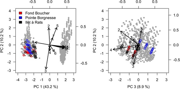
Projection in the parameter space of the combinations of parameter values selected during the calibration all sites confounded (n = 2021).
Arrows indicate parameter loading; numbers designate parameters (coordinates values are displayed on the top and right sides): (1) bleaching model; (2) cyclone model; (3) grazing model; (4) growth rate reduction; (5) otherProportions; (6) prob cover crustose coralline algae; (7) ratio overtop colony; (8) prob grazing macroalgae; (9) prob grazing allopathic macroalgae; (10) prob grazing Halimeda; (11) prob grazing articulated coralline algae; (12) prob grazing crustose coralline. Grey dots represent individual combinations of parameter values. Circles highlight the 20 combinations providing best performance in each site.
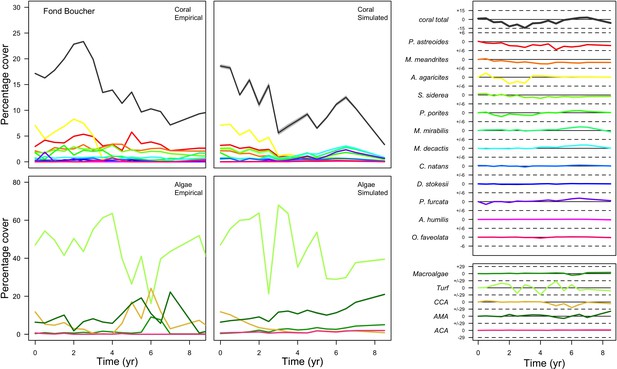
Comparison between empirical and simulated taxa cover for the combination of parameter values providing the best performance for site Fond Boucher.
Solid lines in the simulated time series are the mean percentages cover (averaged over five replicates) and the shaded areas show the standard error. The right panels display the cover difference between simulated and empirical time series.
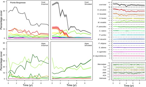
Comparison between empirical and simulated taxa cover for the combination of parameter values providing the best performance for site Pointe Borgnesse.
Solid lines in the simulated time series are the mean percentages cover (averaged over five replicates) and the shaded areas show the standard error. The right panels display the cover difference between simulated and empirical time serie.
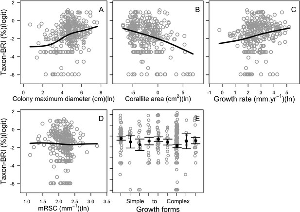
Relationships between the taxon-BRI]0,1[ (logit-transformed) and the five bleaching resistance traits initially selected (n = 304).
Black lines are smoothing splines and are used for visual aid. Growth forms are ranked from the most complex to the simplest: branching, table/plate, corymbose, digitate, laminar, columnar, massive, encrusting long upright, encrusting. Each gray circle represents the trait value averaged by species, the black points are the averaged trait value over all the species by category (E), and the error bars extend to ± one standard error.
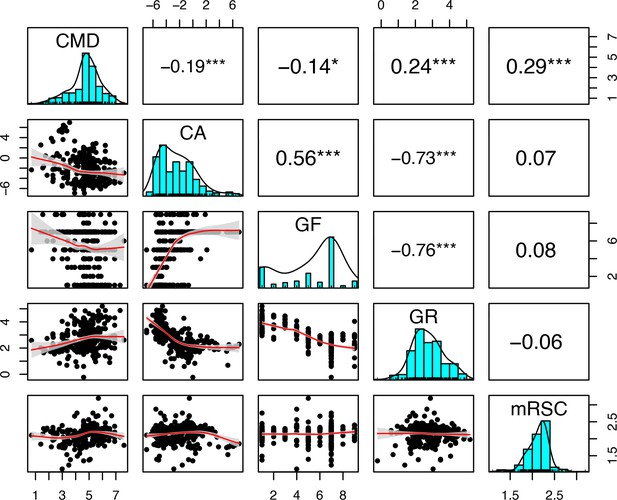
Correlation analyses between the bleaching resistance traits used in the full regression model (n = 304): colony maximum diameter (CMD), coralline algae (CA), growth forms (GF), growth rate (GR), and microscopic reduced scattering coefficient (mRSC).
Growth forms are ranked from the most complex to the simplest: branching, table/plate, corymbose, digitate, laminar, columnar, massive, encrusting long upright, encrusting. Black points represent the trait value averaged by species, the red line is the locally estimated scatterplot smoothing fit and the grey area it 95% confidence interval. The upper panels show the values of the Spearman’s rank correlation coefficient. Asterisks indicate the test statistics’ significance: *p < 0.05; **p < 0.01; ***p < 0.001.
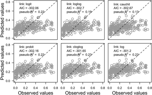
Associations between the observed and predicted values for different versions of the global model.
Each version implements a different link function to estimate the parameter μ (n = 304). Also displayed are the pseudo R2, the Akaike information criterion (AIC) and the identity line.
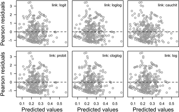
Associations between Pearson’s residuals and predicted values for the different versions of the global model.
Each version implements a different link function to estimate the parameter μ (n = 304).
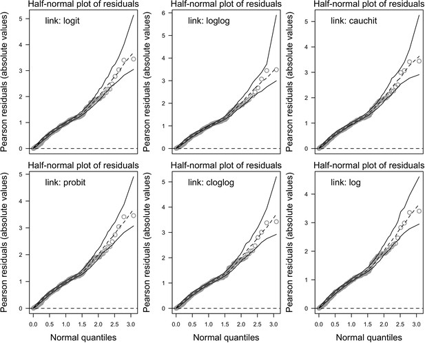
Half-normal plot with simulated envelopes for the different versions of the global model.
Each version implements a different link function to estimate the parameter μ (n = 304).
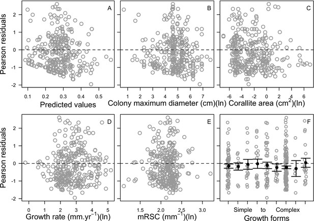
Relationship between Pearson residuals of the averaged ‘subset’ beta regression model and predicted values (A), and each of the potential bleaching resistant traits (B–F) (n = 304).
Growth forms are ranked from the most complex to the simplest: branching, table/plate, corymbose, digitate, laminar, columnar, massive, encrusting long upright, encrusting. Each gray circle represents the trait value averaged by species, the black points are the averaged trait value over all the species by category (E), and the error bars extend to ± one standard error.
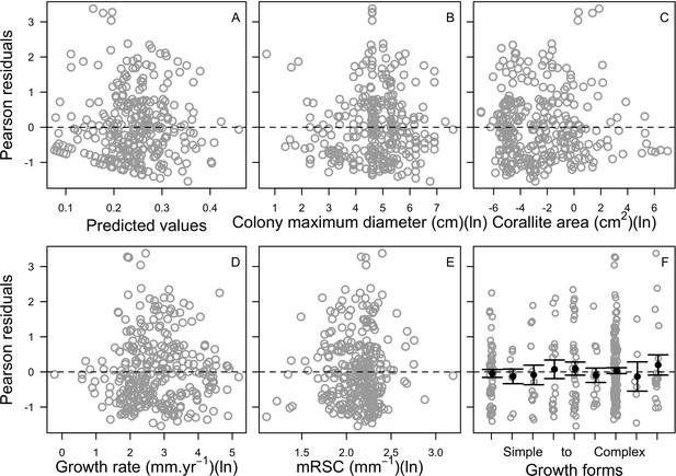
Relationship between Pearson residuals of the averaged ‘full’ beta regression model and predicted values (A), and each of the potential bleaching-resistant traits (B–F) (n = 304).
Growth forms are ranked from the most complex to the simplest: branching, table/plate, corymbose, digitate, laminar, columnar, massive, encrusting long upright, encrusting. Each gray circle represents the trait value averaged by species, the black points are the averaged trait value over all the species by category (E), and the error bars extend to ± one standard error.
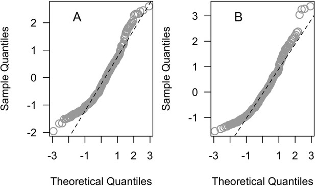
Normal quantile plot of the Pearson residuals of the averages ‘subset’ (A) and the ‘full’ (B) beta regression models (n = 304).
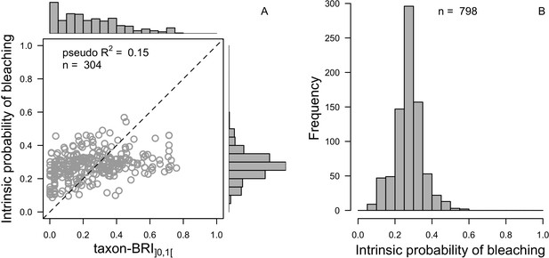
Comparison of distributions between the observed (taxon-BRI]0,1[) and the predicted (intrinsic probability of bleaching) response variable (A) and the extrapolated intrinsic probability of bleaching (n = 798, B) for the averaged ‘subset’ beta regression model.
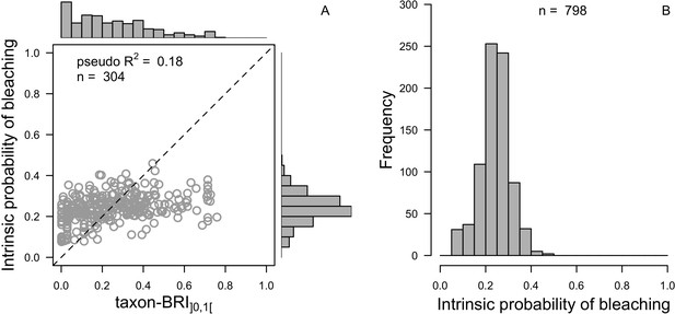
Comparison of distributions between the observed (taxon-BRI]0,1[) and the predicted (intrinsic probability of bleaching) response variable (A) and the extrapolated intrinsic probability of bleaching (n = 798, B) for the averaged ‘full’ beta regression model.
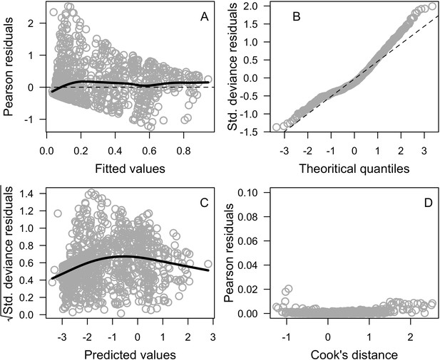
Diagnostic plots of the generalized linear mixed model (n = 1216).
Black lines are smoothing splines and are used for visual aid.
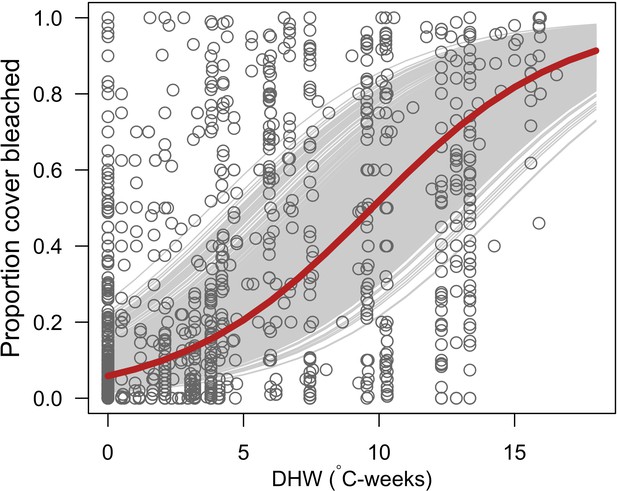
Relationship between the proportion of cover bleached in reefs and degree heating week (DHW).
Grey circles represent individual observations (n = 1216) in a given site at a certain time (Eakin et al., 2010). The grey lines are the logistic regression curves of the general linear mixed model for each combination of sites and time (i.e. random effects; n = 771). The red curve is the logistic regression without random effects (y = 1/(1+exp(2.78–0.29 × DHW))).
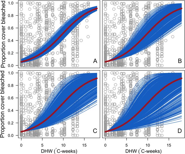
Species-specific logistic bleaching responses with i being independent of DHW (A), dependent of DHW and (B), (C) and (D).
Grey circles are individual sampling proportions of coral cover bleached (n = 1216) from Eakin and colleagues’ (2010) dataset. The solid red line represents the logistic regression fitting these observations (y = 1/(1+exp(2.78-0.29×DHW))). Blue lines represent the response of each 798 coral species.
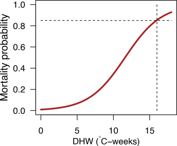
General mortality response of a bleached coral colony as a function of degree-heating weeks (DHW) (y = 1/(1 + exp(−0.4 * (x - 11.6)))).
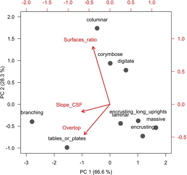
Principal component analysis used to quantify growth form on continuous dimensions.
Grey dots represent growth forms and red arrows represent the load the different process-related variables (see text for details).
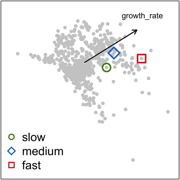
Principal component analysis of the coral functional space (shown with the first two principal components) and the three species selected to assess growth rate and space saturation processes: Acropora pulchra (red square; fast: 65.5 mm.yr−1); A. polystoma (blue diamond; medium: 37.3 mm.yr−1); A. gemmifera (green circle; slow: 12.0 mm.yr−1).
Each grey dot represents one of the 798 species. The black arrow represents the load of the trait growth rate.

Space saturation due to the vegetative growth of a unique coral species in absence of any other processes (colonies are distinguished by different shades of purple).
We took screen shots of the 2 × 2 m2 at different time intervals.
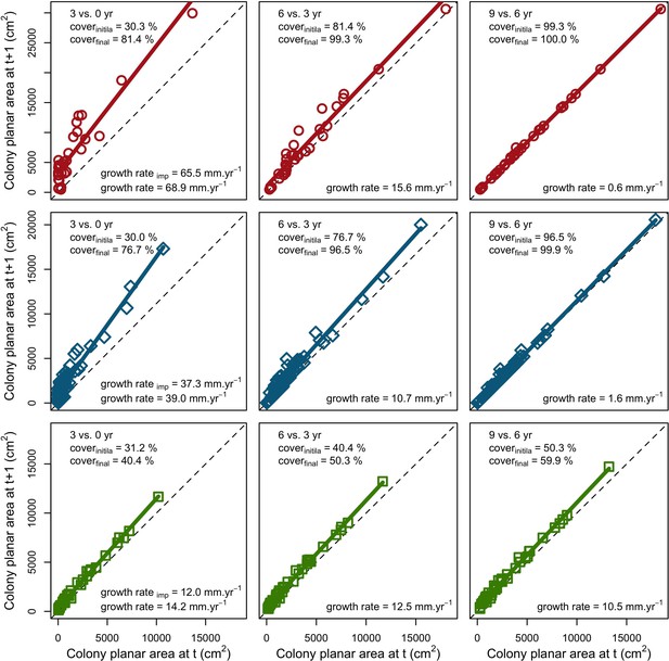
Effect of space saturation on coral colony growth rate saturation for three coral species, growing in a monospecific reef: Acropora pulchra (red square); A. polystoma (blue diamond) and A. gemmifera (green circle).
The implemented growth rate (growth rateimp) corresponds to the values found in the literature. The dashed lines indicate no growth.
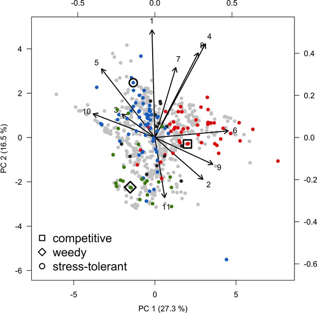
Principal component analysis of the coral functional space (shown with the first two principal components) and the three species selected to assess recruitment rate and space saturation processes: Acropora gemmifera (competitive, red dot in square); Agaricia tenuifolia (weedy, green dot in diamond); Echinophyllia orpheensis (stress-tolerant, blue dot in circle).
Each grey dot represents one of the 798 species, colored dots are species classified either as competitive (red), weedy (green), stress-tolerant (blue) generalist (black) by Darling et al. (2012). Arrows indicate trait loadings; numbers correspond to: (1) aggressiveness; (2) colony maximum diameter; (3) corallite area; (4) egg diameter; (5) polyp fecundity; (6) growth rate; (7) mode of larval development; (8) sexual system; (9) bleaching probability; (10) growth form PC1; (11) growth form PC2.
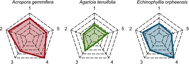
Functional characteristics of the three species selected to assess recruitment rate and space saturation processes (from left to right: competitive in red, weedy in green and stress-tolerant in blue).
Each vertex of the web corresponds to a trait: (1) colony maximum diameter (log10); (2) egg diameter (mm); (3) colony fecundity (no. eggs.cm−2, log10); (4) mode of larval development; (5) growth rate (log10). The colored polygons situate the trait value of the species in the range of values spanned by the 798 species, with highest values at the extremities and lowest values near the center of the web.
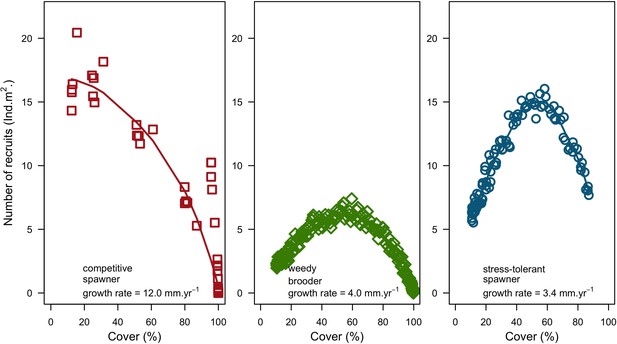
Recruitment rate and space saturation for three coral species, growing in a monospecific reef: Acropora gemmifera (competitive, red dot in square); Agaricia tenuifolia (weedy, green dot in diamond); Echinophyllia orpheensis (stress-tolerant, blue dot in circle).
Each symbol indicates the cover and number of recruits measured at a given time interval. Simulations were replicated five times. Trend lines are shown for visual aid. Also displayed is the species radial growth rate.
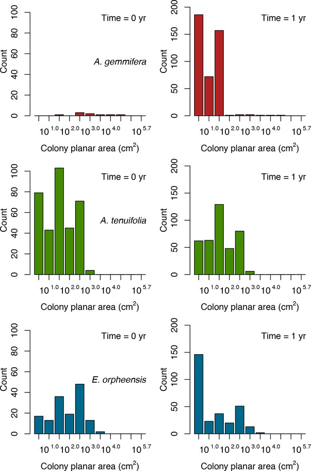
Initial colony size-frequency distributions of the three species grown in a monospecific reef for the recruitment rate and space saturation simulations.
Frequencies were averaged over five replicates.
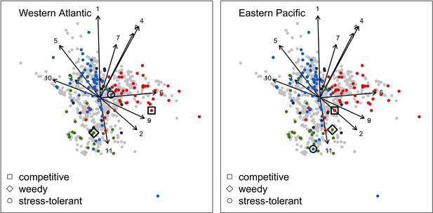
Principal component analyses of the coral functional space (shown with the first two principal components) and the three species selected to assess response to disturbances, larval connectivity, grazing and competition.
Species from the Western Atlantic (left) are: Acropora palmata (competitive, red dot in square); Madracis pharensis (weedy, green dot in diamond); Orbicella annularis (stress-tolerant, blue dot in circle). Species from the Eastern Pacific (right) are: Pocillopara elegans (competitive, red dot in square); P. damicornis (weedy, green dot in diamond); Porites lutea (stress-tolerant, blue dot in circle). Each grey dot represents one of the 798 species, colored dots are species classified either as competitive (red), weedy (green), stress-tolerant (blue) or generalist (black) by Darling et al. (2012). Arrows indicate trait loadings; trait numbers correspond to: (1) aggressiveness; (2) colony maximum diameter; (3) corallite area; (4) egg diameter; (5) polyp fecundity; (6) growth rate; (7) mode of larval development; (8) sexual system; (9) bleaching probability; (10) growth form PC1; (11) growth form PC2.
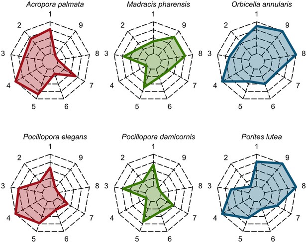
Functional characteristics of the species selected to assess recruitment rate and space saturation processes (the Western Atlantic and Eastern Pacific species are at the top and bottom, respectively; from left to right: competitive in red, weedy in green and stress-tolerant in blue).
Each vertex of the web corresponds to a trait: (1) colony maximum diameter (log10); (2) egg diameter (mm); (3) colony fecundity (no. eggs.cm−2, log10); (4) mode of larval development (i.e. one for spawner, zero for brooder); (5) growth rate (log10); (6) aggressiveness; (7) bleaching susceptibility; (8) growth for PC1 (i.e. resistance to hydrodynamics disturbances and capacity to overtop), (9) growth form PC2 (i.e. 3D to 2D surface ratio). The colored polygons situate the trait value of the species in in the range of values spanned by the 798 species, with highest values at the extremities and lowest values near the center of the web.
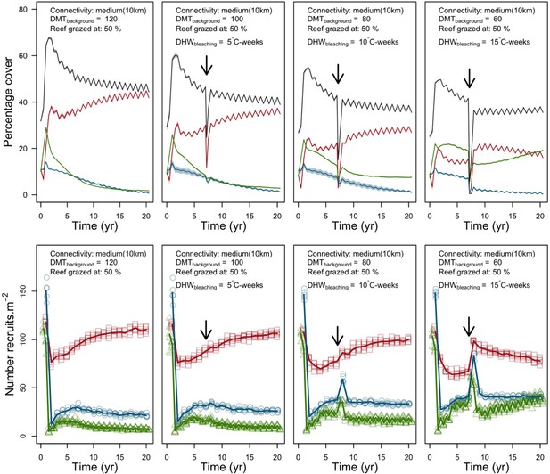
Evolution of cover (top) and number of recruits (bottom) of the three coral species from Western Atlantic (red for the competitive Acropora palamata, green for the weedy Madracis pharensis, blue for the stress-tolerant Orbicella annularis and black for total coral cover) for different disturbance regimes.
The black arrow indicates when the bleaching event occurred. Solid lines represent mean values over five replicates; shaded areas at the top show ± SE; individual symbols at the bottom show the number of recruits at a given time for one replicate.
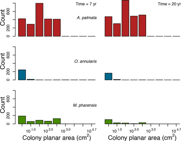
Colony size-frequency distributions of the Western Atlantic species at the lowest wave exposure (DMTbackground = 120) and with no thermal disturbance (DHWbleaching = 0 C°-weeks).
Colonies with a colony planar area = 1 cm2 are not displayed.
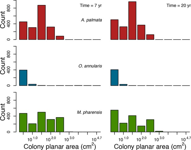
Colony size-frequency distributions of Western Atlantic species at the highest wave exposure (DMTbackground = 60) and thermal disturbance (DHWbleaching = 15 C°-weeks).
Colonies with a colony planar area = 1 cm2 are not displayed.
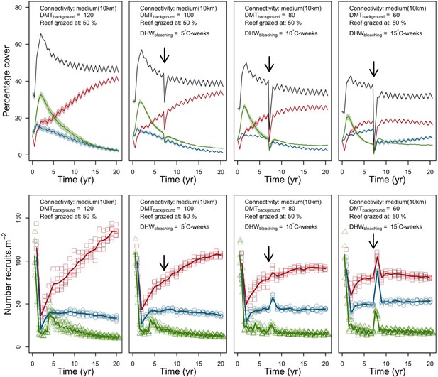
Evolution of the cover (top) and the number of recruits (bottom) of the three coral species from Eastern Pacific (red for the competitive Pocillopara elegans, green for the weedy Pocillopora damicornis, blue for the stress-tolerant Porites lutea and black for total coral cover) for different disturbance regimes.
The black arrow indicates when the bleaching event occurred. Solid lines represent mean values over five replicates; shaded areas at the top show ± standard error; individual symbols at the bottom show the number of recruits at a given time for one replicate.
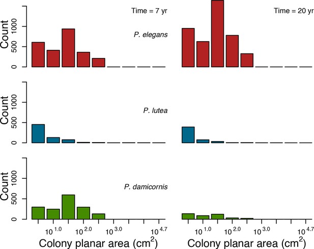
Colony size-frequency distributions of the Eastern Pacific species at the lowest wave exposure (DMTbackground = 120) and with no thermal disturbance (DHWbleaching = 0 C°-weeks).
Colonies with a colony planar area = 1 cm2 are not displayed.
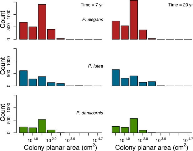
Colony size-frequency distributions of the Eastern Pacific species at the highest wave exposure (DMTbackground = 60) and thermal disturbance (DHWbleaching = 15 C°-weeks).
Colonies with a colony planar area = 1 cm2 are not displayed.
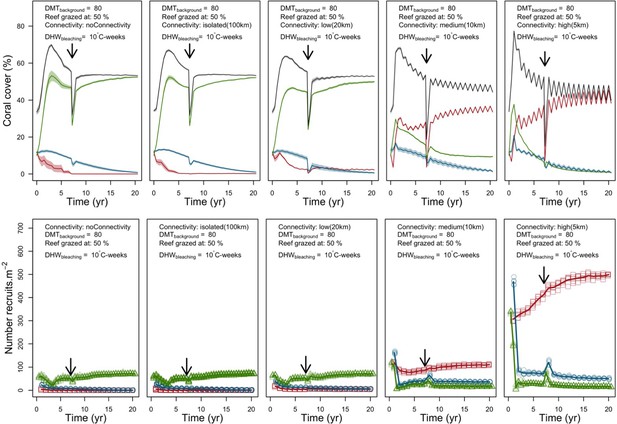
Evolution of cover (top) and number of recruits (bottom) of the three coral species from Western Atlantic (red for the competitive Acropora palamata, green for the weedy Madracis pharensis, blue for the stress-tolerant Orbicella annularis and black for total coral cover) for different larval connectivity levels.
The black arrow indicates when the bleaching event occurred. Solid lines represent mean values over five replicates; shaded areas at the top show ± standard error; individual symbols at the bottom show the number of recruits at a given time for one replicate.
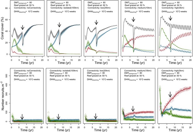
Evolution of the cover (top) and the number of recruits (bottom) of the three coral species from Eastern Pacific (red for the competitive Pocillopara elegans, green for the weedy Pocillopora damicornis, blue for the stress-tolerant Porites lutea and black for total coral cover) for different for different larval connectivity levels.
The black arrows indicates when the bleaching event occurred. Solid lines represent mean values over five replicates; shaded areas at the top show ± standard error; individual symbols at the bottom show the number of recruits at a given time for one replicate.
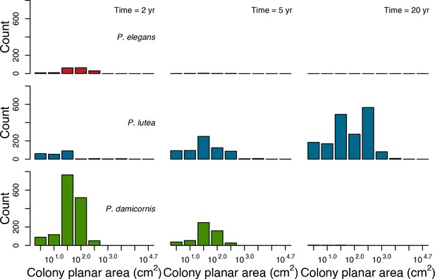
Colony size-frequency distributions of the Eastern Pacific species with no larval connectivity.
Colonies with a colony planar area = 1 cm2 are not displayed.
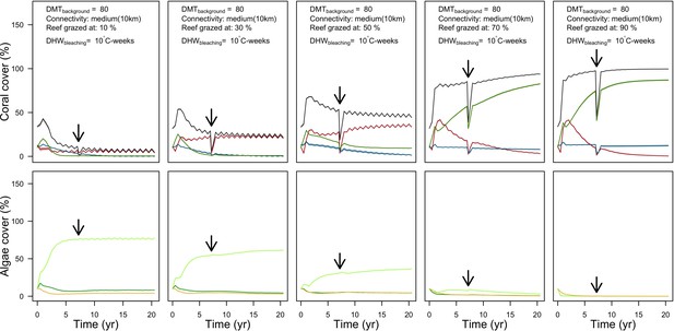
Evolution of cover of the three coral species from Western Atlantic (top: red for the competitive Acropora palamata, green for the weedy Madracis pharensis, blue for the stress-tolerant Orbicella annularis and black for total coral cover) and algae (bottom: light green for turf, dark green for macroalgae and orange for CCA) for different grazing intensities.
The black arrow indicates when the bleaching event occurred. Solid lines represent mean values over five replicates; shaded areas at the top show ± standard error.
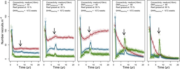
Evolution number of recruits of the three coral species from Western Atlantic (red for the competitive Acropora palamata, green for the weedy Madracis pharensis, blue for the stress-tolerant Orbicella annularis and black for total coral cover) for different grazing intensities.
The black arrow indicates when the bleaching event occurred. Solid lines represent mean values over five replicates; individual symbols show the number of recruits at a given time for one replicate.
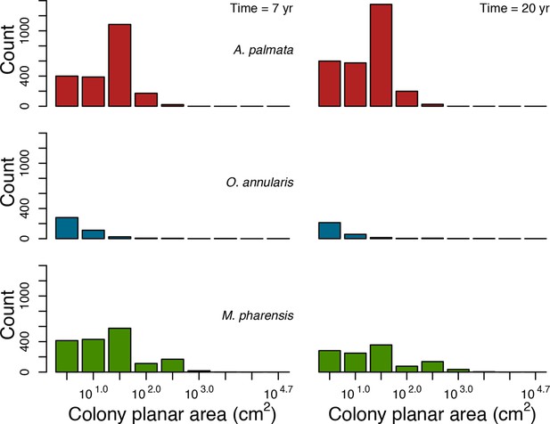
Colony size-frequency distributions of the Western Atlantic species at lowest grazing pressure (i.e. 10%).
Colonies with a colony planar area = 1 cm2 are not displayed.
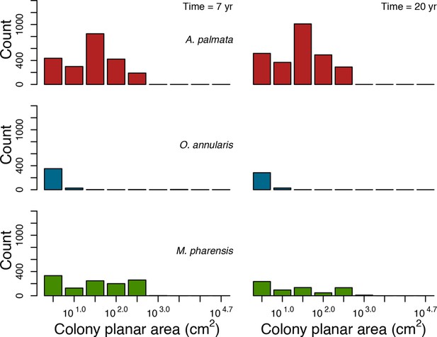
Colony size-frequency distributions of the Western Atlantic species at intermediate grazing pressure (i.e. 50%).
Colonies with a colony planar area = 1 cm2 are not displayed.
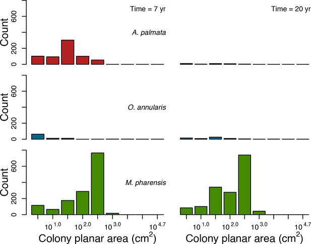
Colony size-frequency distributions of the Western Atlantic species at highest grazing pressure (i.e. 90%).
Colonies with a colony planar area = 1 cm2 are not displayed.
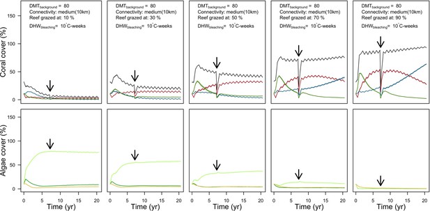
Evolution of cover of the three coral species from Eastern Pacific (red for the competitive Pocillopara elegans, green for the weedy Pocillopora damicornis, blue for the stress-tolerant Porites lutea and black for total coral cover) and algae (bottom: light green for turf, dark green for macroalgae and orange for CCA) for different grazing intensities.
The black arrow indicates when the bleaching event occurred. Solid lines represent mean values over five replicates; shaded areas at the top show ± standard error.
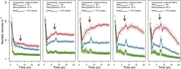
Evolution number of recruits of the three coral species from Eastern Pacific (red for the competitive Pocillopara elegans, green for the weedy Pocillopora damicornis, blue for the stress-tolerant Porites lutea and black for total coral cover) for different grazing intensities.
The black arrows indicates when the bleaching event occurred. Solid lines represent mean values over five replicates; individual symbols show the number of recruits at a given time for one replicate.
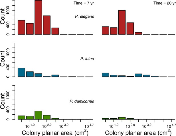
Colony size-frequency distributions of the Eastern Pacific species at highest grazing pressure (90%).
Colonies with a colony planar area = 1 cm2 are not displayed.
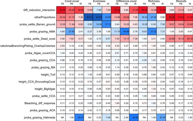
Influence (%) of each model parameter (rows) on each of the five response variables (columns), for each site: Fond Boucher (FB), Pointe Borgnesse (PB) and Ilet à Rats.
Red and blue colours represent positive and negative relationships between parameters and response variables, respectively. Colour saturation indicates the amount of influence of parameters.

Relationship between the parameter growth rate reduction interaction and evenness predicted by the fitted boosted regression trees (fitted function) for each site (FB = Fond Boucher; PB = Pointe Borgnesse; IR = Ilet à Rats).
Fitted functions are centred by subtracting their mean from each value.
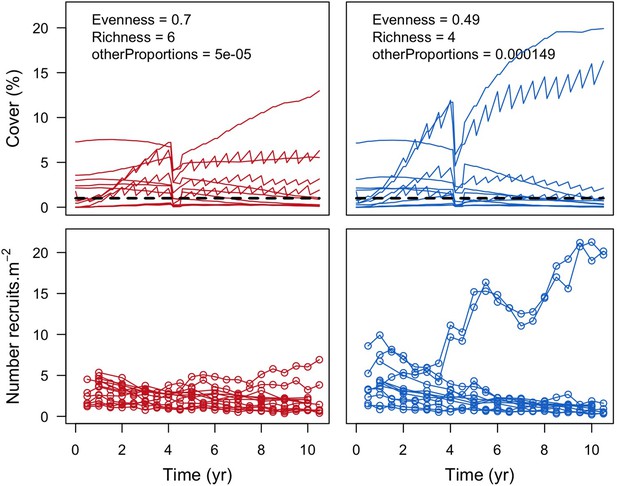
Example of a comparison of the effect of lower (left panels, red) and higher (right panels, blue) values of otherProportions on individual coral species cover (top panels) and number of recruits m−2 at Fond Boucher.
Each line represents the cover or number of recruits of one coral species (n = 12 species). The black dashed line in the top panels shows the 1% cover threshold below which species were not accounted for richness (at 10.5 years).
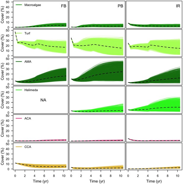
Comparison of algae cover between sites (FB = Fond Boucher; PB = Pointe Borgnesse; IR = Ilet à Rats).
Each line represents the algal cover of one simulation; the dashed black line shoes the averaged cover over all the simulations (n = 1000).
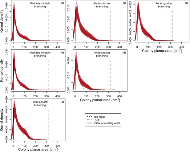
Examples of colony size distributions of branching species by sites (FB = Fond Boucher; PB = Pointe Borgnesse; IR = Ilet à Rats) at 8 years.
Each red line represents a species’ colony size distribution in one simulation; each plot shows 100 distributions that we randomly selected among the 1000 simulations. Horizontal black lines display the minimum colony planar area necessary to achieve for a colony to overtop the corresponding algae (CCA = crustose coralline algae; the line for big algae falls outside of the plots).
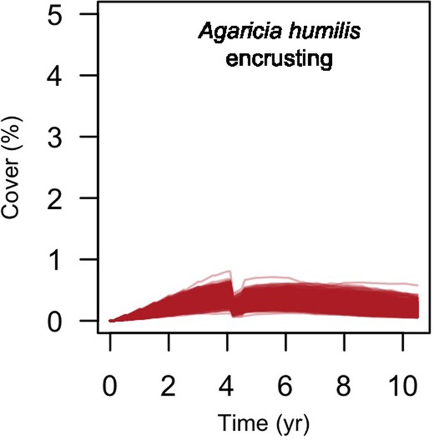
Cover of the encrusting coral species present at Fond Boucher.
Each line represents the cover of one simulation (n = 1000).
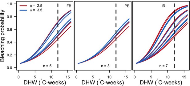
Bleaching probability of the most abundant species for the two extreme ϕ in each site (FB = Fond Boucher; PB = Pointe Borgnesse; IR = Ilet à Rats).
We calculated the mean abundance at 10.5 years over the 1000 simulations and selected the n species with a mean percentage cover >1%. The vertical dashed line shows the intensity of the thermal perturbation imposed in the simulations (12°C-weeks).
Tables
The 11 functional traits we used to implement ecological processes in the model.
| Traits | Related processes and details |
|---|---|
| Age at maturity (yr) | The minimum age required for a coral colony to reproduce (Appendix 2: §7.2.1.1.a) |
| Aggressiveness (0 to 100) | Spatial direct competition for space between coral species; the trait is only used for species not considered in the Precoda et al., 2017 study on probability of species-pair interactions (Appendix 1: §1.2) |
| Colony max diameter (cm) | Initial colony size distributions (Appendix 2: §5.2.2); colony fecundity (for the species with small colonies; Appendix 2: §7.2.1.1.b); bleaching (Appendix 2: §7.4.2.1; Appendix 4); colony vegetative growth (to define maximum planar area; Appendix 2: §7.5.1) |
| Corallite area (cm2) | Colony fecundity (Appendix 2: §7.2.1.1.b); bleaching (Appendix 2: §7.4.2.1; Appendix 4) |
| Egg diameter (mm) | Time to motility of coral larvae (§7.2.1.1.d) |
| Polyp fecundity | Colony fecundity (Appendix 2: §7.2.1.1.b) |
| Growth form | Formation of reef rugosity (Appendix 2: §7.1.2.2); colony fecundity (Appendix 2: §7.2.1.1.b); dislodgement (Appendix 2: §7.3.1.2); spatial competition (overtopping; Appendix 2: §7.5) |
| Growth rate (mm.yr−1) | Bleaching (Appendix 2: §7.4.2.1; Appendix 4); vegetative growth (Appendix 2: §7.5.1) |
| Mode of larval development | Coral reproduction (Appendix 2: §7.2.1.1.a) |
| Microscopic reduced scattering coefficient (µS,m, mm−1) | Bleaching (Appendix 2: §7.4.2.1; Appendix 4) |
| Sexual system | Colony fecundity (Appendix 2: §7.2.1.1.b) |
Empirical data and models we used to implement ecological processes in the model.
| Processes/variables | Comments | References |
|---|---|---|
| Colony size (initialization) | We used colony size distributions measured for eleven species and maximum colony diameter to define colony size distributions for each species (Appendix 2: §5.2.2) | E. H. Meesters and R. P. M. Bak, personal communication, May 2017 |
| Herbivorous fish density supported by the reef rugosity | We used an empirical model to determine the density of herbivore fish present in the reef as a function of reef rugosity (Appendix 2: §7.1.2.2) | Bozec et al., 2013 |
| Grazing intensity due to herbivorous fish density | We defined a model using empirical data to determine the surface of the reef grazed as a function of herbivorous fish density (Appendix 2: §7.1.2.2) | Williams and Polunin, 2001 |
| Polyp maturity in colonies | We defined a model from models established empirically to determine the proportion of mature polyps in a colony as a function of colony planar area using data for eight species (Appendix 2: §7.2.1.1.b) | Álvarez-Noriega et al., 2016 |
| Larval competency | We used a model established empirically to determine time to motility of coral larvae as a function of egg diameter (Appendix 2: §7.2.1.1.d) | Figueiredo et al., 2013 |
| Larval retention | We used models established empirically to determine the proportion of competent larvae remaining in the reef as a function of time to motility and water retention time (Appendix 2: §7.2.1.1.d) | Figueiredo et al., 2013 |
| Larval competency loss | We defined a model from models established empirically to determine the proportion of external competent larvae settling on the focal reef as a function of the distance travelled (Appendix 2: §7.2.1.2.b) | Connolly and Baird, 2010 |
| Larval post-settlement survival | We defined a model using empirical data to determine the proportion of surviving settled larvae as a function of time (Appendix 2: §7.2.1.3.b) | Ritson-Williams et al., 2016 |
| Colony dislodgement | We used models established empirically to determine if a colony is dislodged as a function of colony growth form, planar area and the intensity of the hydrodynamic disturbance (Appendix 2: §7.3.1.2.a) | Madin and Connolly, 2006 |
| Survival of dislodged branching colonies | We defined a model using a model established empirically to determine the proportion of a dislodged branching colony that survives dislodgement (Appendix 2: §7.3.1.2.b) | Highsmith et al., 1980 |
| Coral bleaching | We used the empirically established bleaching-response index to determine species bleaching susceptibility from functional traits (Appendix 2: §7.4.2; Appendix 4) | Swain et al., 2016b |
| Coral competition | We used species-pair probabilities of interaction outcomes established from mix-effect models and a review of empirical data (Appendix 2: §7.5.2.2.a) | Precoda et al., 2017 |
| Coral-algae competition | We defined probabilities of interaction outcomes using proportions of interaction won and lost between coral species and the different functional group of algae implemented measured experimentally (Appendix 2: §7.5.3) | Brown et al. (2017) and K. T. Brown, personal communication, October 2017 |
Summary of the sources and the methods of compilation of the functional-trait data.
We downloaded all trait information from coraltrait.org between 30 March 2017 and 19 April 2018 (taxon-BRI: Bleaching Response Index).
| Traits | Source(s) | No. sp. | Used in model | Used for imputation | Comments |
|---|---|---|---|---|---|
| Age at maturity (yr) | Coral Trait Database | 3 | Yes | No | This trait is not used in the trait in-filling process because it is defined for too few species |
| Aggressiveness (0 to 100) | Abelson and Loya, 1999 Connell et al., 2004 Dai, 1990 Lang, 1973 Logan, 1984 Sheppard, 1979 | 116 | Yes | Yes | Values 0 and 100 correspond to the lowest and highest possible aggressiveness, respectively (see §1.2 for details) |
| Coloniality | Coral Trait Database | 743 | No | Yes | Used to increase the number of predictors in the imputation random forest procedure |
| Colony max diameter (cm) | Coral Trait Database | 307 | Yes | Yes | We considered the maximum value in case of duplicated species |
| Corallite area (cm2) | Coral Trait Database | 712 | Yes | Yes | Obtained from ‘corallite width maximum’ and ‘corallite width minimum’; we calculated the average when both values were available |
| Egg diameter (mm) | (Figueiredo et al., 2013) Coral Trait Database | 25 | Yes | Yes | We obtained values from the coral trait database from ‘egg size’ (two species) and ‘mature egg diameter’ (four species); values were averages when possible |
| Polyp fecundity | Coral Trait Database | 13 | Yes | Yes | Values obtained from ‘polyp fecundity’ (10 species) and ‘mesentery fecundity’ (three species); we averaged values when possible |
| Growth form | Coral Trait Database | 791 | Yes | Yes | We used ‘growth form typical’. We grouped under ‘branching’ the ‘open’ and ‘closed branching’ and ‘hispidose’; ‘massive’ also comprises ‘submassive’ |
| Growth rate (mm.yr−1) | Coral Trait Database | 125 | Yes | Yes | We converted radial to linear/diametral measurements |
| Mode of larval development | Coral Trait Database | 312 | Yes | Yes | Pocillopora ankeli and P. damicornis can be both brooder and spawner, but are considered brooder in the model |
| Microscopic reduced scattering coefficient (µS,m, mm−1) | Marcelino et al., 2013; Swain et al., 2016a | 93 | Yes | Yes | - |
| Taxon-BRI (0–100) | Marcelino et al., 2013; Swain et al., 2016a; Swain et al., 2016b | 304 | No | No | We removed observations for which only the genera was known and for non-scleractinian coral |
| Sexual system | Coral Trait Database | 306 | No | Yes | To increase the number of predictors in the imputation random-forest procedure. This trait is particularly well-conserved (Brandt and McManus, 2009) |
| Total number of species | 798 |
References used to define the aggressiveness ranking index per species (CI: Coral Index).
| References | Metrics | Original no. of taxa | Final no. of species | Remarks |
|---|---|---|---|---|
| Lang, 1973 | Ranking number based on number of subordinates | 27 | 22 | |
| Sheppard, 1979 | CI | 26 | 22 | |
| Logan, 1984 | Number of subordinates | 17 | 15 | Paired-interactions showing opposite result between field and lab experiment were not considered |
| Dai, 1990 | Classification in five categories based on CI | 76 | 76 | |
| Abelson and Loya, 1999 | Ranking number based on frequency of wins and losses and composition of losing and winning species | 33 | 30 | |
| Connell et al., 2004 | % of winning interactions | 13 | 11 | |
| Total number of species: | 147 | 116 |
Grid-cell agent attributes, state variables (*) and other variables.
| Variable name | Description |
|---|---|
| context | The 'context' (a Java object that encapsulates the agents and projections; it is static, and all the agents belong to the same context). |
| grid | The 'grid', a spatial Projection associated to the Contextand allowing to place and locate the agents spatially (it is static, and all the agents are part of the same Grid). |
| x * | The x coordinate of the agent in the grid (static). |
| y * | The y coordinate of the agent in the grid (static). |
| substrateCategory * | First categorization of the agents: BarrenGround for barren ground and sand; Algae for algae; Coral for corals. Value are imported from data/functionalTraitDF_model.csv |
| substrateSubCategory * | Second categorization of the agents: BarrenGround for barren ground and sand; Macroalgae, AMA, Halimeda, Turf, ACA and CCA for macroalgae, allopathic macroalgae, Halimeda spp., turf, articulated coralline algae and crustose coralline algae, respectively; BleachedCoral, DeadCoral, LiveCoral for bleached, dead and living corals, respectively. Value imported from data/functionalTraitDF_model.csv |
| species * | Third categorization of the agents: BarrenGround for barren ground; sand for sand; Macroalgae, AMA, Halimeda, Turf, ACA and CCA for macroalgae, allopathic macroalgae, Halimeda spp., turf, articulated coralline algae and crustose coralline algae, respectively; coral species names for corals (e.g., Acanthastrea_brevis). Value imported from data/functionalTraitDF_model.csv |
| age * | Age (yr) of living agents. |
| age_maturity * | Species traits (see Appendix 1—table 1) Value imported from data/functionalTraitDF_model.csv |
| aggressiveness * | |
| bleaching_probability * | |
| coloniality * | |
| colony_maximum_diameter * | |
| corallite_area * | |
| egg_diameter * | |
| fecundity_polyp * | |
| growth_form * | |
| mode_larval_development * | |
| reduced_scattering_coefficient * | |
| sexual_system * | |
| size_maturity * | |
| growth_rate * | The maximum radius rmax within which an agent can convert neighboring agents (see §7.5.1) |
| correction_coeff_polypFecundity * | A coefficient to apply to small species (colony_maximum_diameter < 16.7 cm) when determining the proportion of mature polyps in the colony (see §7.2.1.1.b). |
| timeRecoveryBleaching * | Time (yr) remaining before the agent totally recovers from bleaching (see §7.4). |
| IDNumber * | The identification number; unique to each colony and shared by the agents forming a same colony. |
| red * | The Red Green Blue (RGB) colour code to represent each benthic entity. Value imported from data/functionalTraitDF_model.csv |
| green * | |
| blue * | |
| canIGrow * | Boolean variable used to allow or forbid an agent to grow. |
| haveIbeenConverted * | Boolean variable used to forbid an agent to grow during the Growth procedure (Figure 2) if it has already been converted (i.e., overgrown) by another agent during the same Growth procedure. |
| haveIbeenGrazed * | Boolean variable used to forbid an algae agent to overgrow another non-algae agent if the latter has been grazed during the Grazing procedure of the same time step (Figure 2). |
| planar_area_colony | The planar area (cm2) of the colony formed by the agent (the value equals the number of agents forming the colony). |
| newRecruit * | Boolean variable used to indicate if the agent is a new recruit (i.e., if it settled during the Coral reproduction procedure of the present time step; Figure 2). |
| size_UpDated * | Boolean variable used to indicate if the agent’s planar_area_colony has been updated during a procedure of colony size update (i.e., after each disturbance and at the end of a time step; Figure 2). |
Parameters of the linear regression models for skew and bias expressed as a function of maximum colony diameter (log10) (n = 31).
| Model | Parameters | Estimate | SE | R2 | p-Value |
|---|---|---|---|---|---|
| skew | Intercept | 0.62 | 0.022 | 0.86 | <0.001 |
| Slope | 0.14 | 0.010 | <0.001 | ||
| bias | Intercept | 0.59 | 0.094 | 0.96 | <0.001 |
| Slope | −1.20 | 0.044 | <0.001 |
Probabilities of being grazed of each algal functional group implemented in the model.
We considered several values for calibration (Appendix 3). Bold values are the ones providing best fit in at least one of the three Caribbean sites. More than one bold value are shown when different values maximized the fit in different sites. No bold values are shown when none of the values tested improved the fit.
| Functional groups | Probability of being grazed | Reasoning |
|---|---|---|
| MA | 0.3; 0.5; 0.7 | Thicker structure |
| AMA | 0.3; 0.5 | Thicker structure, strong secondary metabolites |
| Halimeda | 0.3; 0.5; 1.0 | Thicker structure (calcareous), strong secondary metabolites |
| ACA | 0.5; 0.7; 1.0 | Thick structure (calcareous) |
| Turf | 1.0 | Thin structure |
| CCA | 0.05; 0.1; 0.25; 0.5; 0.75 | Harder structure (calcareous), encrusting |
-
MA: macroalgae; AMA: allelopathic macroalgae; Halimeda: Halimeda spp.; ACA: articulate coralline algae; CCA: crustose coralline algae
Parrot fish density and body length (total length ≥4 cm) collected on the fore reef zone of Glovers Atoll by Bozec et al. (2013) and values for a and b parameters of the from the length-weight relationships (LWR) and available from FishBase (Froese and Pauly, 2014).
| Species | Mean density (indiv. 120 m−2) | Mean body length (cm) | A | B |
|---|---|---|---|---|
| Scarus iserti | 4.28 | 9.8 | 0.01096 | 3.02 |
| Sparisoma aurofrenatum | 2.41 | 13.4 | 0.01072 | 3.12 |
| Sparisoma viride | 1.12 | 24.0 | 0.01380 | 3.04 |
| Sparisoma chrysopterum | 0.37 | 26.7 | 0.01072 | 3.09 |
| Sparisoma rubripinne | 0.12 | 28.4 | 0.00933 | 3.04 |
| Scarus taeniopterus* | 0.04 | 16.7 | 0.01096 | 3.02 |
| Scarus vetula | 0.02 | 27.8 | 0.01445 | 3.04 |
| Scarus coelestinus | <0.01 (0.005)† | 40.0 | 0.01622 | 3.05 |
-
*Values for a and b for Scarus taeniopterus were not available so we chose values for Scarus iserti because the two species have similar maximum total and common lengths.
†We attributed a density of 0.005 indiv.120 m-2 for Scarus coelestinus
Formulae and values used to calculate the three dimensional surface area of colonies depending on their growth form (McWilliam et al., 2018b).
Note that we corrected the formula for laminar (M. McWilliam, personal communication, July 2019).
| Growth from | Formula surface area | Parameter values |
|---|---|---|
| Branching* | | |
| Tabular | See branching | |
| Laminar | ||
| Massive | - | |
| Corymbose | See branching | |
| Digitate | See branching | |
| Columnar | See branching | |
| Encrusting long upright | Encrusting + branching | |
| Encrusting | - |
-
Parameters are: colony radius (r); branch radius (rb); branch height (hb); number of branches per cm2 (Nb).
* Coefficient values were obtained by averaging values for 'complex' and 'simple' branching.
Parameter values for the models defining the probability of a polyp to be fecund as a function of colony planar surface area (Álvarez-Noriega et al., 2016).
| Species | Growth form | Intercept | Slope | n | ||||
|---|---|---|---|---|---|---|---|---|
| LCI | Median | UCI | LCI | Median | UCI | |||
| A. hyacinthus | tabular | 4.022 | 5.908 | 8.345 | 0.889 | 1.602 | 2.477 | 24 |
| A. cytherea | tabular | 0.446 | 1.023 | 1.657 | 0.107 | 0.462 | 0.841 | 24 |
| A. digitifera | digitate | 7.309 | 11.507 | 17.142 | 1.252 | 2.277 | 3.572 | 24 |
| A. humilis | digitate | 9.477 | 14.999 | 22.269 | 1.649 | 2.833 | 4.339 | 24 |
| A. nasuta | corymbose | 7.782 | 14.074 | 22.922 | 1.296 | 2.791 | 4.753 | 24 |
| A. spathulata | corymbose | 5.933 | 9.496 | 14.107 | 0.973 | 1.838 | 2.916 | 24 |
| G. pectinata | massive | 0.802 | 7.036 | 14.169 | −0.594 | 0.771 | 2.126 | 20 |
| G. retiformis | massive | 2.796 | 4.966 | 7.423 | 0.376 | 0.883 | 1.450 | 20 |
| Average | - | - | 8.626 | - | - | 1.682 | - | - |
Parameter values for the different models expressing the proportion of larvae retained in the reef (ps) as a function of time to motility (tm, in days) and retention time (Figueiredo et al., 2013).
| Retention time (d) | α | β | γ | ρ |
|---|---|---|---|---|
| 16.3 | 0.801 | −0.222 | - | - |
| 10.24 | 0.768 | −0.247 | - | - |
| 7.66 | 0.741 | −0.267 | - | - |
| 6.97 | 0.731 | −0.274 | - | - |
| 4.69 | 0.180 | - | 0.545 | 1.354 |
| 2.14 | 0.090 | - | 0.557 | 2.740 |
| 1.50 | 0.050 | - | 0.551 | 3.400 |
| 1.21 | 0.031 | - | 0.536 | 3.800 |
| 0.90 | 0.014 | - | 0.501 | 4.500 |
| 0.70 | 0.006 | - | 0.461 | 5.100 |
Proportion of larvae from the remote reef reaching the focal reef (prf) depending on the separation distance.
| Distance between reefs | prf |
|---|---|
| High (5 km) | 0.5 |
| Medium (10 km) | 0.1 |
| Low (20 km) | 0.01 |
| Isolated (100 km) | 0.001 |
| Isolated (200 km) | 0.0001 |
| Not connected | 0.0 |
Parameter values for the different models predicting the proportion of larvae alive (Palive) and competent (Pcompetent) as a function of time (Connolly and Baird, 2010).
| Species | Competency model (Pcompetent) | Survival model (Palive) | |||
|---|---|---|---|---|---|
| a | b | tc | λ | ν | |
| Acropora millepora | 0.180 | 0.050 | 3.239 | 0.043 | 0.57 |
| Acropora valida | 0.220 | 0.031 | 0.000 | 0.019 | 0.46 |
| Acropora gemmifera | 0.390 | 0.145 | 3.471 | 0.067 | 1.00 |
| Goniastrea retiformis | 0.580 | 0.096 | 0.000 | 0.087 | 1.00 |
| Platygyra daedalea | 0.390 | 0.099 | 2.937 | 0.060 | 0.72 |
| Average | 0.352 | 0.084 | 1.929 | 0.055 | 0.75 |
-
tc: Development time required before acquisition of competence can begin, in days.
Proportion of larvae remaining alive and competent (pac) as a function of the distance between the remote and the focal reef.
We defined the traveling time assuming 0.15 m.s−1 current velocity and alignment of the reefs in the current direction. Also displayed is the corresponding number of larvae settling by squared meter of the focal reef (Lsr) and the corresponding values of the model parameter connectivity.
| Distance between reefs | Connectivity | Duration journey (d) | pac | Lsr (m−2) |
|---|---|---|---|---|
| 5 km | ‘high (5 km)’ | 0.39 | 0.40 * | 35000.00 |
| 10 km | ‘medium (10 km)’ | 0.77 | 0.40 * | 7000.00 |
| 20 km | ‘low (20 km)’ | 1.54 | 0.40 * | 700.00 |
| 100 km | ‘isolated (100 km)’ | 7.72 | 0.38 | 66.50 |
| 200 km | ‘isolated (200 km)’ | 15.43 | 0.17 | 2.98 |
| ∞ | “noConnectivity | - | 0.0 | 0.00 |
| - | ‘connectivityCSV’ | - | - | - |
-
* At these distances, the larvae have reached the focal reef before being competent. We attributed the maximum proportion as we assumed these larvae remain and settle in the focal reef.
Proportions of larvae settling, metamorphosing and surviving (Pss) in different laboratory experiments.
| Pss (%) | Substratum type | Duration | No. coral sp. | Reference |
|---|---|---|---|---|
| 36 to 87 | 5 CCA sp. | 1 day | 3 | Morse et al., 1988 |
| 67 to 91 | 4 CCA and 1 ACA sp. | 8 days | 1 | Heyward and Negri, 1999 |
| 27 | Rubble | |||
| 0 to > 60 | Coral skeleton | |||
| 64.2; 57.2; 47.1 | Tile | 2, 30, 60 days | 2 | Nishikawa et al., 2003 |
| 81.7, 59.9, 13.1 | 0, 20, 40 days | |||
| 24.2 | 1 CCA sp. | 240 days | 2 | Harrington et al., 2004 |
| 20.1 | Tile | |||
| 0 | four other CCA sp. | |||
| 0 to 80 | 2 CCA sp., rubble | 24 hr | 2 | Golbuu and Richmond, 2007 |
| 0 to 18 | 2 CCA sp. | 6 weeks | 2 | Ritson-Williams et al., 2010 |
-
CCA: crustose coralline algae; ACA: articulated coralline algae
Probabilities of successful coral larvae settlement on different substrata.
| Substratum | pls | Justification |
|---|---|---|
| Barren ground dead coral CCA | 0.5 | We chose this mid value for all the suitable substratum types because of the high diversity of coral specificity toward CCA species and other substratum (Birrell et al., 2008), and the wide ranges of settlement success (Appendix 2—table 11), and insufficient knowledge. |
| Sand | 0.0 | Sand does not provide a stable substratum for coral larvae to metamorphose |
| Alive coral | 0.0 | Corals feed on larvae (Fabricius and Metzner, 2004) |
| Bleached coral | 0.0 | Bleached corals rely on heterotrophy to compensate for the loss of the symbiont (Grottoli et al., 2006) |
| Macroalgae turf AMA | 0.0 | Pre-emption of space, and release of deleterious or lethal chemicals impede larvae metamorphosis (Birrell et al., 2008) |
| ACA | 0.0 | ACA do not provide a stable substratum for coral larvae to metamorphose |
| Halimeda | 0.0 | Halimeda is ephemeral so larvae settling die through shading (Nugues and Szmant, 2006) |
-
CCA: crustose coralline algae; AMA: allelopathic macroalgae; ACA: articulate coralline algae
Parameter values of the least-squares regression model we established based on Ritson-Williams et al. (2016)'s results: y = Intercept + Slope × 1/x ( Appendix 2—figure 11, Appendix 2—figure 12).
| Parameters | Estimate | SE | P-value |
|---|---|---|---|
| Intercept | 10.3 | 8.30 | 0.235 |
| Slope | 43.3 | 15.67 | 0.015 |
Model parameters determining the colony shape factor of a colony as a function of its size and growth form (Madin et al., 2014).
Values below the dashed lines were determined arbitrarily (see text, Appendix 2—figure 13).
| Morphology | β | α | n |
|---|---|---|---|
| Branching | 0.79 | 8.34 | 73 |
| Table_or_plate | 0.39 | 4.47 | 76 |
| Corymbose | 0.16 | 2.28 | 78 |
| Digitate | −0.04 | 1.25 | 68 |
| Massive | −0.23 | −0.94 | 86 |
| Laminar | 0.27 | 3.80 | - |
| Columnar | 0.20 | 3.00 | - |
| Encrusting_long_upright | 0.00 | 1.40 | - |
| Encrusting | 0.00 | 1.00 | - |
Models and parameter values defined to determine the proportion of algal cover removed as a function of dislodgement mechanical threshold for each functional group of algae (Appendix 2—figure 15).
| Functional groups | Proportion algae cover removed (Par, %) | ||
|---|---|---|---|
| DMT ≤ 10 | 10 < DMT < α | α ≤ DMT | |
| MA AMA ACA Halimeda | 100 | α = 130 | 0 |
| Turf | 90 | α = 110 | 0 |
| CCA | 80 | α = 90 | 0 |
-
DMT: dislodgement mechanical threshold; MA: macroalgae; CCA: crustose coralline algae; AMA: allelopathic macroalgae; ACA: articulate coralline algae
Examples of coral growth and calcification rates reduction after a bleaching event.
| Species | Growth rate reduction (%) | Bleaching event | Time post bleaching | Reference |
|---|---|---|---|---|
| Montastrea annularis | 60 | Nov. 1987, Jamaica, strong | 6 mo. | Goreau and Macfarlane, 1990 |
| Acropora millepora A. hyacinthus | ~100 | Early 1998, GBR, strong | 9 mo. | Baird and Marshall, 2002 |
| Montastraea annularis | 40 to 80 | Sept. 1995, Jamaica, ? | 5 to 7 mo. | Mendes and Woodley, 2002 |
| Porites compressa | 89* 100* 67* | Experiment | 1.5 mo. 4 mo. 8 mo. | Rodrigues and Grottoli, 2006 |
| Montipora capitata | 80* 80* 27* | Experiment | 1.5 mo. 4 mo. 8 mo. | Rodrigues and Grottoli, 2006 |
-
*Calcification rate.
Examples of different effects of bleaching events on coral reproduction.
| Species | Effect on reproduction | Bleaching event | Time post bleaching | Reference | |
|---|---|---|---|---|---|
| Acropora millepora A. hyacinthus | % reduction of fecund colonies | - 54 - 7 | Early 1998, GBR, strong | 9 months | Baird and Marshall, 2002 |
| Montastraea annularis | No gametogenesis completed for severely bleached colonies | Sept. 1995, Jamaica | 1 year | Mendes and Woodley, 2002 | |
| Acropora aspera A. humilis A. millepora A. nobilis A. palifera A. pulchra A. valida Montipora digitata M. spp. Symphyllia spp. | % reduction of polyps fecundity / % reduction of reproductive polyps | 63/59 100/100 −24/8 33/33 66/71 34/14 55/59 77/85 100/100 100/100 | March 1998, GBR, strong | 6 weeks | Ward et al., 2000 |
| Acropora aspera A. millepora A. nobilis A. pulchra A. valida | % reduction of polyps fecundity / % reduction of reproductive polyps | 53/50 51/66 24/54 11 / −31 92/100 | March 1998, GBR, strong | 9 months | Ward et al., 2000 |
| A. nasuta | % reduction of fertilization rate | 55 | 1998, Japan, strong | 1 year | Omori et al., 2001 |
| M. annularis | No gametogenesis completed | Summer 1987, Caribbean | 1 year | Szmant and Gassman, 1990 | |
-
GBR: Great Barrier Reef.
Parameters and rules involved in the overtopping process of a branching or plating colony when growing over a coral colony of a patch of algae.
| Parameters | Value | Rule for overtopping |
|---|---|---|
| ratioAreaBranchingPlating_ OvertopColonies | 2 (value calibrated; Appendix 3) | |
| height_BigAlgae (i.e. macroalgae, ACA, AMA, Halimeda) | 30 cm | |
| height_Turf | 10 cm | |
| height_CCA_EncrustingCoral | 2 cm |
-
So: planar surface area of the overtopping branching or plating colony; Su: planar surface area of the overtopped colony; CCA: crustose coralline algae; ACA: articulated coralline algae; AMA: allopathic macroalgae algae.
Functional groups of algae, their competitive outcome probability when competing with corals (based on K. T. Brown, personal communication, October 2017) and radial growth rates.
| Functional group | Description | Probability of winning against corals | Radial growth rate (mm.yr−1) |
|---|---|---|---|
| Macroalgae (MA) | Forms 30 cm high canopy (e.g., Sargassum, Hydroclathrus) | 0.70 | 150 |
| Halimeda spp. | Calcified and non-aggressive macroalgae; forms 30 cm high canopy | 0.15 | 150 |
| Allelopathic macroalgae (AMA) | Produces defensive chemicals; forms 30 cm high canopy (e.g. Chlorodesmis) | 0.80 | 150 |
| Turf | Filamentous algae and cycnobacteria; forms 10 cm high canopy | 1.00 | 250 |
| Articulate coralline algae (ACA) | Forms 30 cm high canopy (e.g. Calliarthron tuberculosum) | 0.40 | 21 |
| Crustose coralline algae (CCA) | Encrusting, 2 cm high (e.g., Porolithon onkodes) | 0.10 | 12 |
Description of parameters calibrated and their respective values considered.
| Parameters | Description | Values |
|---|---|---|
| bleaching model | Value of the coefficient φ (see Appendix 4: §2.2): a smaller φ increases the interspecific difference for the probability of bleaching when the thermal stress increases; a larger φ reduces this difference | 2; 3; 4 |
| cyclone model | Value of one of the three hydrodynamic regimes models displayed in Appendix 3—figure 5 | 1; 2; 3 |
| grazing model | Value of one of the four grazing regimes models displayed in Appendix 3—figure 6 | 1; 2; 3; 4 |
| growth rate reduction interaction | Lateral growth rate reduction coefficient to apply when one coral colony or an algae overgrows over other colonies or algae | 2; 3; 4; 6; 8 |
| otherProportions | The coefficient po, which is used to reduce the number of larvae produced by all the colonies present in the reef (Appendix 2: §7.2.1.1.d) | 0.0001; 0.001; 0.01 |
| prob cover crustose coralline algae | Probability that algae overgrow crustose coralline algae | 0.10; 0.25, 0.50; 0.75 |
| ratio overtop colony | Ratio needed for a branching or plating colony to overtop smaller colonies | 1.5; 2; 3 |
| prob grazing macroalgae | Probability of macroalgae being palatable | 0.3; 0.5; 0.7 |
| prob grazing allopathic macroalgae | Probability of allopathic macroalgae being palatable | 0.3; 0.5 |
| prob grazing Halimeda | Probability of Halimeda spp. being palatable | 0.3; 0.5; 1.0 |
| prob grazing articulated coralline algae | Probability of articulated coralline algae being palatable | 0.5; 0.7; 1.0 |
| prob grazing crustose coralline algae | Probability of crustose coralline algae being palatable | 0.05; 0.1; 0.2; 0.3; 1.0 |
Summary of the bleaching resistance traits (predictors) for the averaged beta regression model (from the 65 models of the 95% confidence set).
The relative importance of each predictor is calculated as a sum of the Akaike weights over all of the models in which the term appears.
| Bleaching resistance traits | Relative importance | No. models where present |
|---|---|---|
| ln(colony maximum diameter) | 1.00 | 65 |
| ln(corallite area) | 1.00 | 65 |
| ln(mRSC) | 1.00 | 65 |
| ln(growth rate) | 0.59 | 49 |
| ln(colony maximum diameter): ln(corallite area) | 0.57 | 37 |
| ln(colony maximum diameter): ln(growth rate) | 0.22 | 23 |
| ln(colony maximum diameter)2 | 0.27 | 29 |
| ln(corallite area) 2 | 0.58 | 37 |
| ln(mRSC) 2 | 0.26 | 29 |
| ln(growth rate) 2 | 0.20 | 21 |
Summary statistics of the ten best models (out of 65) belonging to the 95% confidence set (link function: cloglog).
| Df | logLik | AIC | Delta | Weight | |
|---|---|---|---|---|---|
| 1/2/8/9* | 6 | 169.759 | −327.517 | 0.000 | 0.073 |
| 1/2/5/8 | 6 | 169.742 | −327.484 | 0.033 | 0.071 |
| 1/2/3/5/8 | 7 | 170.434 | −326.868 | 0.649 | 0.052 |
| 1/2/5/8/9 | 7 | 170.284 | −326.568 | 0.950 | 0.045 |
| 1/2/3/8/9 | 7 | 170.005 | −326.011 | 1.506 | 0.034 |
| 1/2/3/5/8/9 | 8 | 171.000 | −326.000 | 1.517 | 0.034 |
| 1/2/3/8/9/10 | 8 | 170.948 | −325.896 | 1.622 | 0.032 |
| 1/2/8 | 5 | 167.844 | −325.689 | 1.829 | 0.029 |
| 1/2/3/5/6/8 | 8 | 170.825 | −325.650 | 1.867 | 0.029 |
| 1/2/4/5/8 | 7 | 169.793 | −325.585 | 1.932 | 0.028 |
-
*Each number corresponds to a predictor: ln(colony maximum diameter) (1); ln(corallite area) (2); ln(growth rate) (3); ln(colony maximum diameter)2 (4); ln(corallite area)2 (5); ln(growth rate)2 (6); ln(mRSC)2 (7); ln(mRSC) (8); ln(colony maximum diameter): ln(corallite area) (9).
Estimates of the parameters of the averaged ‘subset’ beta regression model (link function: cloglog).
| Model’s parameters | Estimate | Std. error | Z value | Pr(>|z|) |
|---|---|---|---|---|
| (Intercept) | −1.242 | 1.0273 | 1.209 | 0.227 |
| ln(colony maximum diameter) | 0.187 | 0.1470 | 1.274 | 0.203 |
| ln(corallite area) | −0.123 | 0.0806 | 1.527 | 0.127 |
| ln(mRSC) | −0.668 | 0.8174 | 0.817 | 0.414 |
| ln(growth rate) | 0.024 | 0.2937 | 0.081 | 0.936 |
| ln(colony maximum diameter): ln(corallite area) | 0.024 | 0.0226 | 1.061 | 0.289 |
| ln(colony maximum diameter): ln(growth rate) | 0.063 | 0.0707 | 0.886 | 0.376 |
| ln(colony maximum diameter)2 | 0.001 | 0.0252 | 0.053 | 0.958 |
| ln(corallite area) 2 | −0.001 | 0.0061 | 1.582 | 0.114 |
| ln(mRSC) 2 | 0.135 | 0.3497 | 0.386 | 0.699 |
| ln(growth rate) 2 | −0.034 | 0.0440 | 1.000 | 0.317 |
| phi | 4.267 | 0.3360 | 12.697 | <0.001 |
| Pseudo R2 | 0.122 |
Parameters values of the generalized linear mixed model (binomial distribution and logit link function).
The model as fitted on Eakin et al. (2010)'s dataset.
| Fixed effects | Random effects | |||||
|---|---|---|---|---|---|---|
| Parameters | Estimate | SE | z-value | p-Value | Parameters | Variance |
| α (intercept) | −2.78 | 0.191 | −14.55 | <0.001 | sitej | 0.429 |
| β1 (DHW) | 0.29 | 0.026 | 11.16 | <0.001 | timek | 0.567 |
Description of parameters used in the global sensitivity analysis and their respective ranges for each site (FB = Fond Boucher; PB = Pointe Borgnesse; IR = Ilet à Rats).
| Parameters | Description | Nominal value | Sampling interval |
|---|---|---|---|
| bleaching diff response | Value of the coefficient φ (see Appendix 4: §2.2): a smaller φ increases the interspecific difference for the probability of bleaching when the thermal stress increases; a larger φ reduces this difference | 3 | [2.5,3.5] |
| growth rate reduction interaction | Lateral growth rate reduction coefficient to apply when a coral colony or algae overgrows other colonies or algae | Eight for FB, IR two for PB | [6,10] for FB, IR [1,5] for PB |
| otherProportions | Coefficient po reduces the number of larvae produced by all the colonies present in the reef (see Appendix 2: §7.2.1.1.d) | 0.0001 | [0.00005,0.00015] |
| prob cover crustose coralline algae | Probability that algae overgrow crustose coralline algae | 0.1, 0.25, 0.5, 0.75 | [0,0.05] |
| ratio overtop colony | Ratio needed for a branching or plating colony to overtop smaller colonies | 2 | [1.1,3] |
| prob grazing macroalgae | Probability of macroalgae being palatable | 0.7 for FB, PB 0.5, 0.7 for IR | [0.5,0.9] |
| prob grazing allopathic macroalgae | Probability of allopathic macroalgae being palatable | 0.3, 0.5 for FB, IR 0.3 for PB | [0.2,0.6] for FB, IR [0.1,0.5] for PB |
| prob grazing Halimeda | Probability of Halimeda spp. being palatable | 0.5 for PB 0.3 for IR | [0.2,0.7] for PB [0.1,0.5] for IR |
| prob grazing articulated coralline algae | Probability of articulated coralline algae being palatable | 0.7 | [0.5,0.9] |
| prob grazing crustose coralline algae | Probability of crustose coralline algae being palatable | 0.05, 0.1, 0.2, 0.3 | [0.01,0.1] |
| height big algae* | Height in cm of macroalgae, allopathic macroalgae and articulated coralline algae | 30 | [20,50] |
| height turf * | Height in cm of turf | 10 | [5,15] |
| height crustose coralline algae encrusting coral* | Height in cm of crustose coralline algae, encrusting and encrusting long upright corals | 2 | [0.5,4] |
| prob settle crustose coralline algae* | Probability of a coral larvae to settle successfully on crustose coralline algae agents | 0.5 | [0.2,0.8] |
| prob settle barren ground* | Probability of a coral larvae to settle successfully on barren ground agents | 0.5 | [0.2,0.8] |
| prob settle dead coral* | Probability of a coral larvae to settle successfully on dead coral agents | 0.5 | [0.2,0.8] |
-
*The six additional parameters not considered in the calibration.


