Figures and data in Dynamic metastable long-living droplets formed by sticker-spacer proteins

Figures
Tables
Additional files

10 figures, 1 table and 2 additional files

Figures

Figure 1

Download asset Open asset

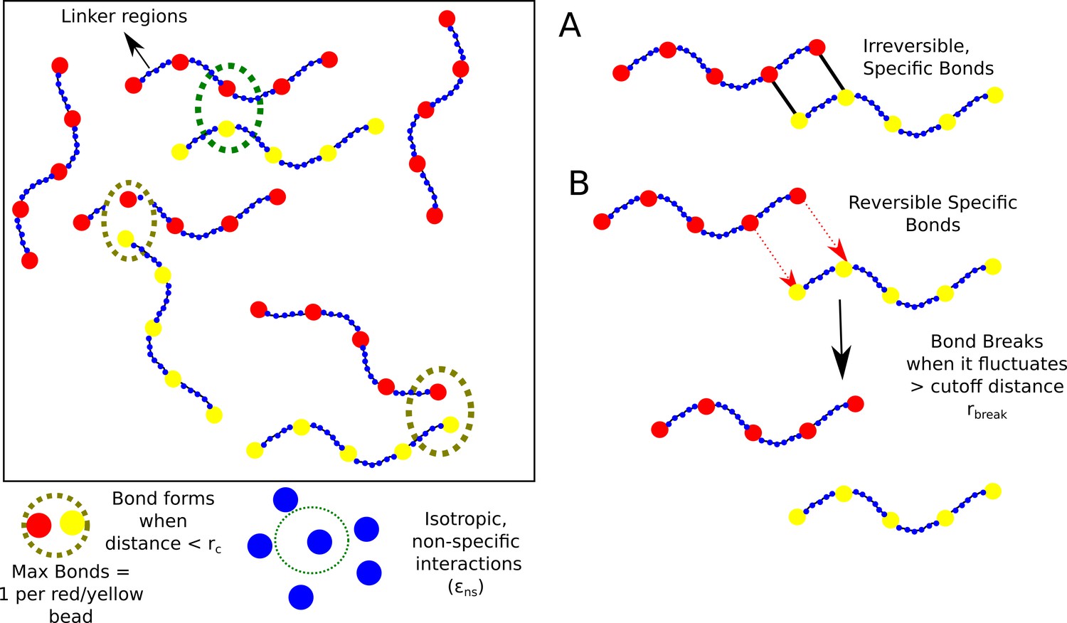
Model.

Schematic of the polymer model for studying phase-separation by multivalent biopolymers.

Figure 2 with 1 supplement

Download asset Open asset

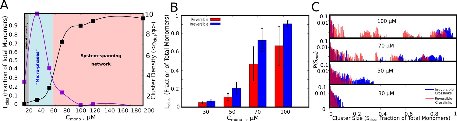
Cluster Sizes in Langevin Dynamics simulations.

(A) Black Curve – The single largest cluster as a function of free monomer concentration (in μM) for irreversible functional interactions. The largest cluster size is shown as a fraction of the total number of monomers in the simulation box. Purple Curve – The mean density of the cluster, $ϕ_{c l u s}$ = $\frac{S_{c l u s}}{(4 / 3) π R_{g}^{3_{c l u s}}}$ , normalized by the bulk density of monomers in the simulation, $ϕ$ = $\frac{S_{c l u s}}{(4 / 3) π R_{g}^{3_{^{'}}}}$ . S_clus and N_tot refer to the size of the cluster and the total number of monomers in the simulation box, respectively. $R_{g}^{c l u s}$ and $R_{g}^{^{'}}$ refer to the radius of gyration of the cluster, and the radius of gyration of proteins in their randomly located initial configuration at the start of the simulation, respectively. The quantity $ϕ_{c l u s}$ / $ϕ$ shows the degree of enrichment of polymer chains within the cluster upon self-assembly. The smooth curves are plotted as a guide to the eye, using the cspline curve fitting. (B) Comparison of the mean sizes of the single largest cluster for reversible and irreversible specific interactions, for varying free monomer concentrations. (C) Cluster size distributions for varying free monomer concentrations for reversible and irreversible specific interactions. Darker shades of red in the distributions indicate verlapping regions of the distribution while the blue and light red shades indicate regions with no overlap in the presence and absence of breakable interactions. The linker stiffness for the self-assembling polymer chains in this plot is 2 kcal/mol while the strength of inter-linker interaction is 0.1 kcal/mol (per pair of interacting beads). The mean and distributions of the largest cluster sizes were computed using 500 different configurations from five independent simulation runs of 16 μs.

Figure 2—source data 1 Compressed zip file containing the source data for cluster sizes and cluster size distributions (along with raw unprocessed data) plotted in Figure 2.: https://cdn.elifesciences.org/articles/56159/elife-56159-fig2-data1-v2.zip
Download elife-56159-fig2-data1-v2.zip

Figure 2—figure supplement 1

Download asset Open asset

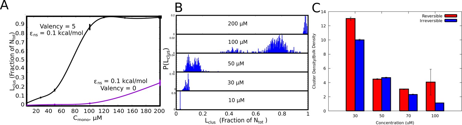
Cluster Sizes in Langevin Dynamics simulations.

(A) The single largest cluster as a function of free monomer concentration (in μM). The largest cluster size is shown as a fraction of the total number of monomers in the simulation box. The smooth curves are plotted as a guide to the eye, using the cspline curve fitting. The vertical bars represent the standard error. (B) Cluster size distributions for increasing free monomer concentrations. The linker stiffness for the self-assembling polymer chains in this plot is two kcal/mol while the strength of inter-linker interaction is 0.1 kcal/mol (per pair of interacting beads). The simulations were performed for an instantaneous bond formation assumption ( $P_{f o r m}$ =1). (C) Comparison of mean intra-cluster density ( $ϕ_{c l u s}$ / $ϕ$ ) as a function of concentration for reversible and irreversible crosslinks.

Figure 3 with 1 supplement

Download asset Open asset

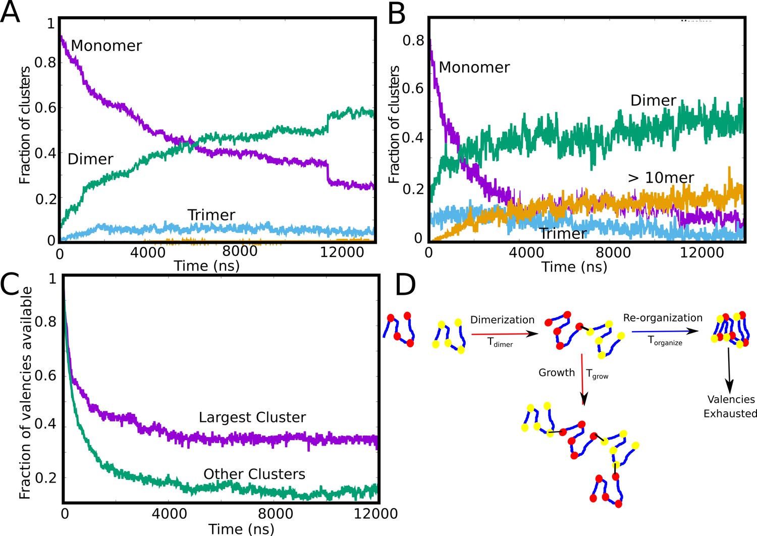
Tracking cluster formation at early timescales.

A and B show the temporal evolution of specific contacts for a free monomer concentration of 10, and 50 μM, respectively. For a low concentration of 10 μM, there is an initial decrease in the monomer population (purple curve) which is concomitant with an increase in the dimer population. A negligible fraction of the clusters is in the form of large-mers (size > = 10, orange curve) at these low concentration since the available valencies for growth are consumed by the smaller aggregated species. An increase in concentration from 10μM to 50μM results in an increase in the large-mer (orange curve, 50 μM) population as the monomer fraction decreases during the simulation. A higher free monomer concentration allows the larger clusters to grow due to consumption of free monomers (with unsatisfied valencies) before they get converted into smaller clusters (dimers, trimers) with satisfied valencies. (C) Time evolution of available valencies within the single largest cluster and outside the single largest cluster, for a $C_{m o n o}$ of 50 μM, $ϵ_{n s}$ of 0.1 kcal/mol and linker bending rigidity of 2 kcal/mol. (D) A schematic figure showing the possible mechanisms of cluster growth and arrest and the competing timescales that could punctuate the process.

Figure 3—source data 1 Compressed zip file containing the source data for temporal evolution of different species (dimer,trimer,monomer etc) for different concentrations plotted in Figure 3.: https://cdn.elifesciences.org/articles/56159/elife-56159-fig3-data1-v2.zip
Download elife-56159-fig3-data1-v2.zip

Figure 3—figure supplement 1

Download asset Open asset

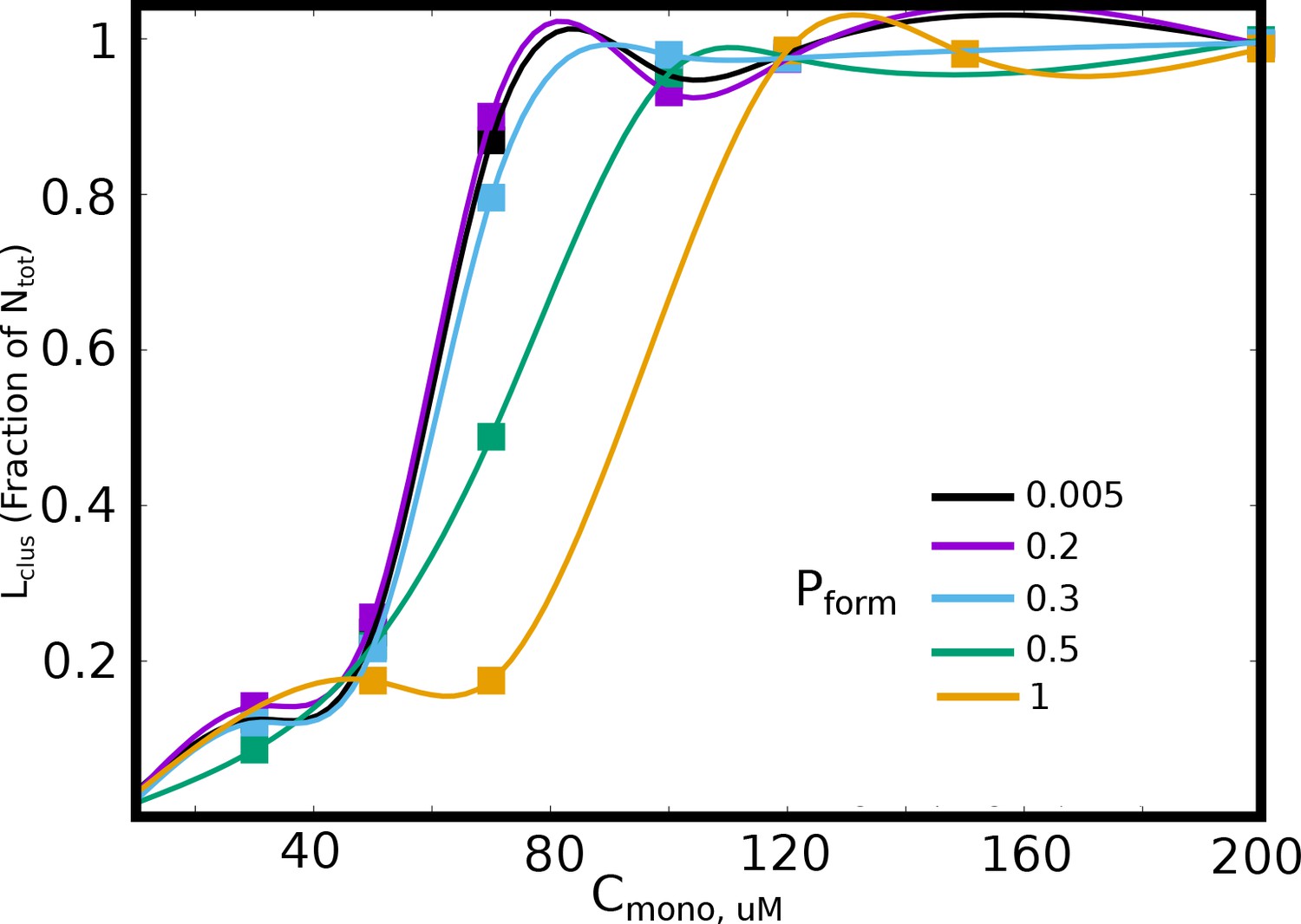
The size of the largest cluster, for different values of bond formation probability, $P_{f o r m}$ .

A lower $P_{f o r m}$ results in a slower arrest of the clusters, and thereby results in increased cluster sizes for smaller free monomer concentration, $C_{m o n o}$ .

Figure 4

Download asset Open asset

Factors influencing the key timescales.

(A) The mean first passage time for the first specific interaction between a pair of polymer chains as a function of the bulk density, $ϕ$ , (see Table 1 for definition). (B) The mean first passage time for a pair of polymer chains to exhaust all the available valencies within the dimer.

Figure 4—source data 1 Compressed zip file containing the source data for Figure 4.: https://cdn.elifesciences.org/articles/56159/elife-56159-fig4-data1-v2.zip
Download elife-56159-fig4-data1-v2.zip

Figure 5 with 3 supplements

Download asset Open asset

Linkers as modulators of self-assembly propensity.

(A) The size of the largest cluster for flexible linker regions( $κ$ =2 kcal/mol) with varying inter-linker interaction strength (black curve, 0.1 kcal/mol and purple curve, 0.5 kcal/mol). Sticky inter-linker interactions result in smaller cluster sizes. (B). Purple Curve – Mean Radius of gyration for the individual-polymer chains (< $R_{g}^{c h a i n}$ >) within a self-assembled cluster as a function of increased inter-linker interactions. Black Curve— Mean density of the clusters as a function of inter-linker interaction strength. (C) The mean re-organization times, $T_{e x h a u s t - v a l e n c y}$ as a function of linker-stiffness, for different values of inter-linker interaction strengths.

Figure 5—source data 1 Compressed zip file containing the source data for largest cluster size, density of the cluster and radius of gyration of constituent chains, for different values of $ϵ_{n s}$ plotted in Figure 5.: https://cdn.elifesciences.org/articles/56159/elife-56159-fig5-data1-v2.zip
Download elife-56159-fig5-data1-v2.zip

Figure 5—figure supplement 1

Download asset Open asset

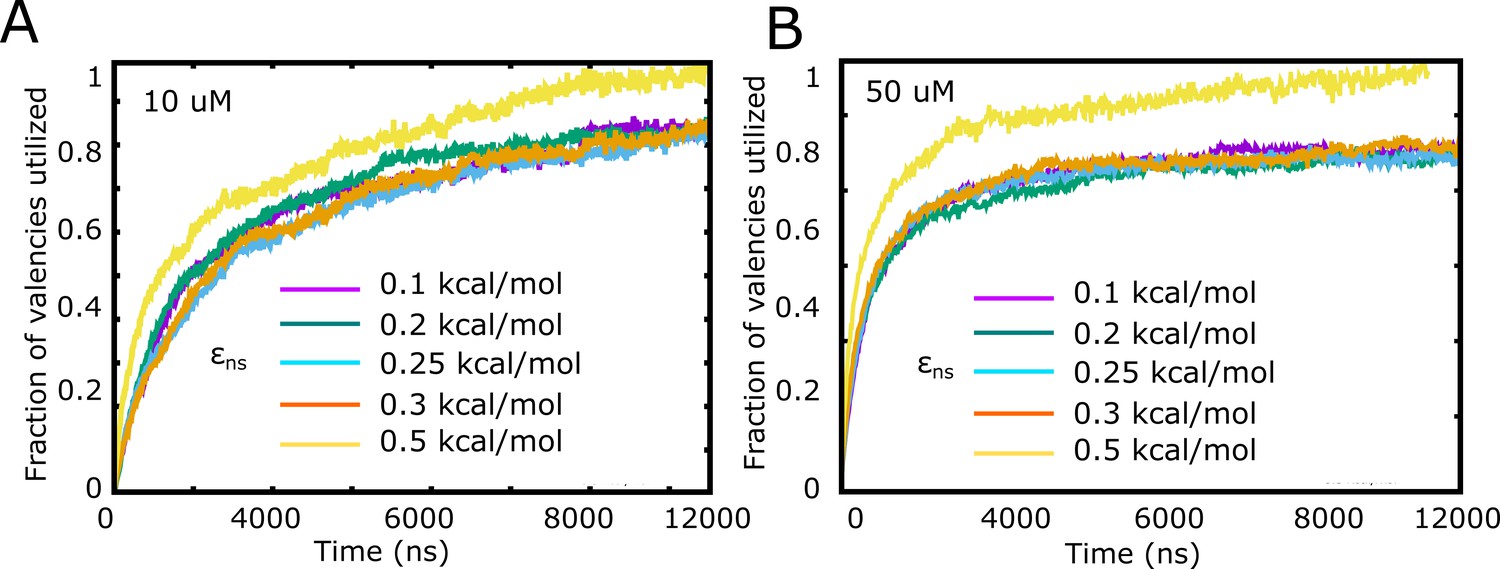
Fraction of valencies utilized as a function of increasing inter-linker interaction strength, for (A) 10 μM and (B) 50 μM free monomer concentration.

Figure 5—figure supplement 2

Download asset Open asset

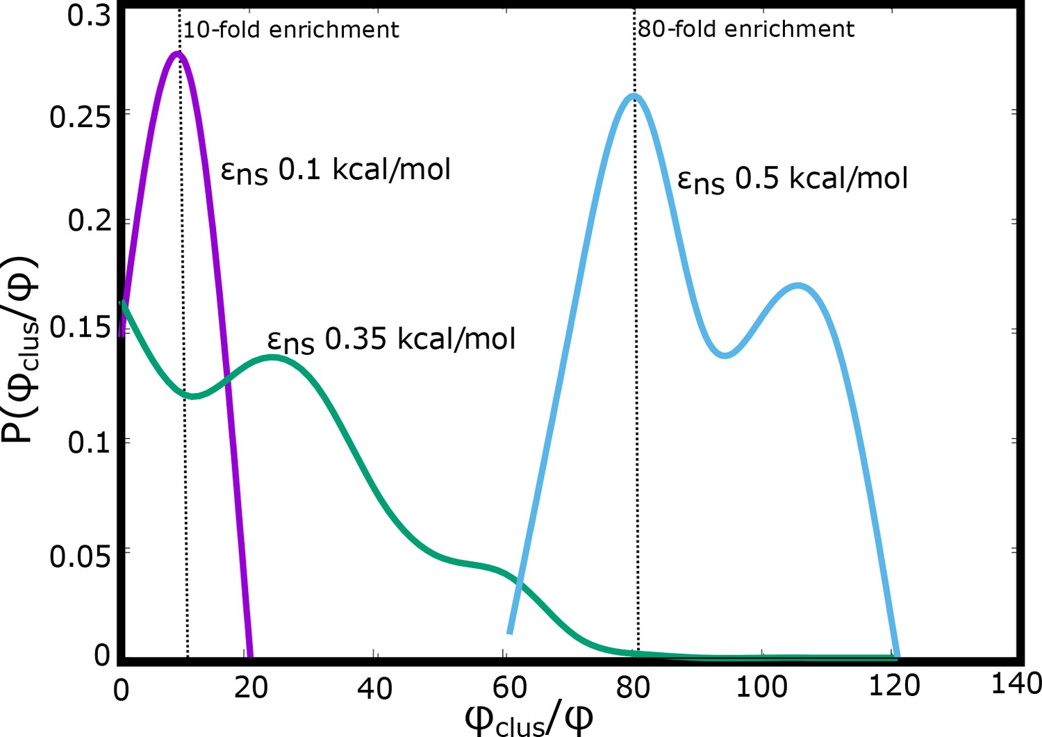
The probability of finding clusters with varying densities (normalized by the bulk densities) for different values of inter-linker interactions.

As the inter-linker interactions increase, the degree of enrichment can go from 10-fold to 100-fold.

Figure 5—figure supplement 3

Download asset Open asset

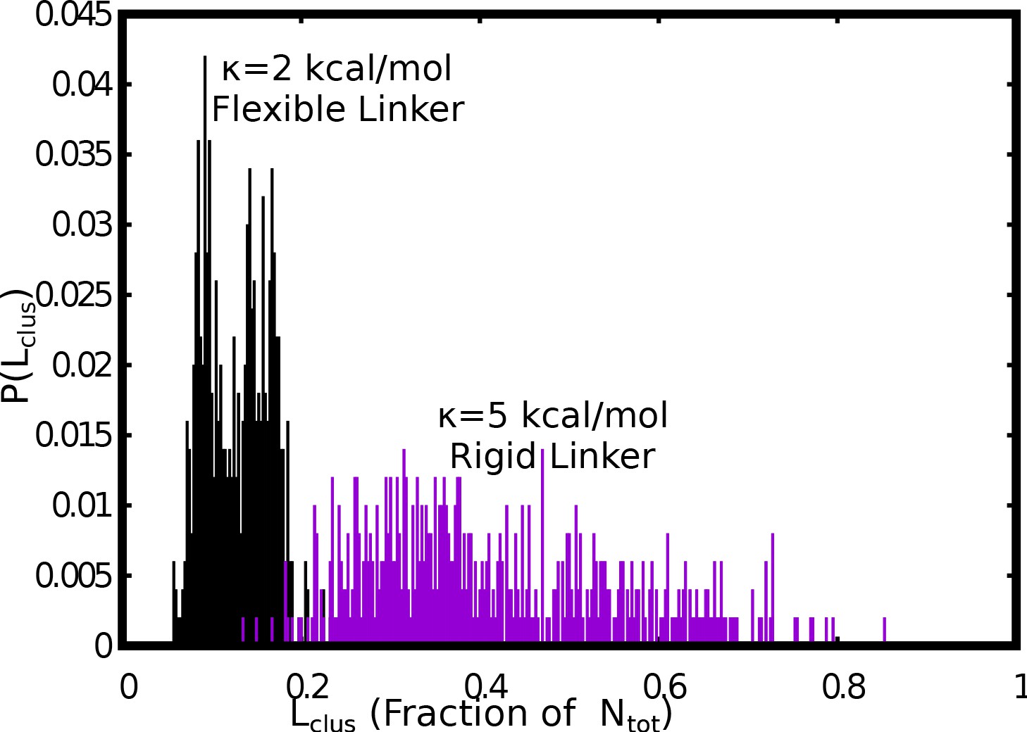
Comparision between the size distributions of the largest cluster, for flexible ( $κ$ =2 kcal/mol) versus stiff ( $κ$ =5 kcal/mol) linker regions.

The free monomer concentration used for this plot was 50 μM and a weak interlinker interaction strength of $ϵ_{n s}$ = 0.1 kcal/mol was used.

Figure 6

Download asset Open asset

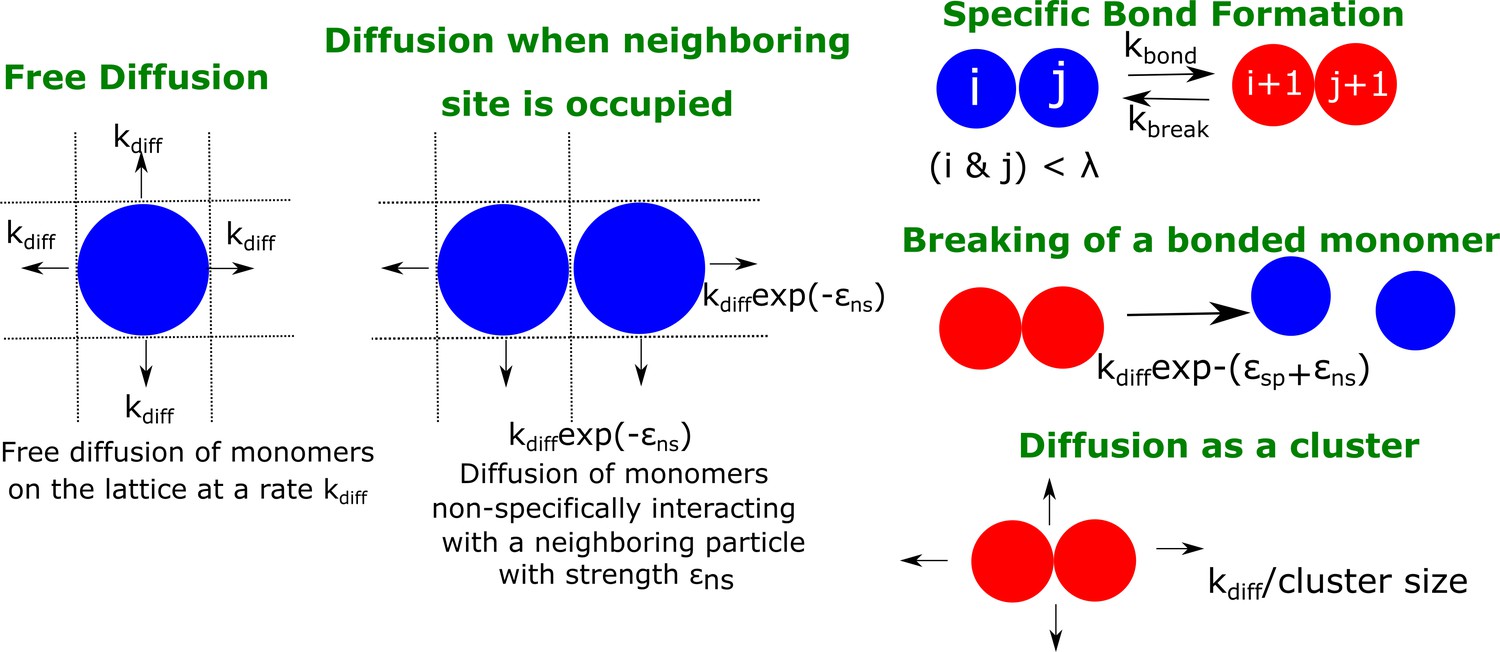
A schematic figure detailing the different rates in our phenomenological kinetic model simulated using the Gillespie algorithm.

The particles on the lattice can diffuse freely (when there are no neighboring particles) with a rate $k_{d i f f}$ . In the presence of a neighboring particle, a non-specifically interacting monomer can diffuse away with a rate $k_{d i f f} ϵ_{n s}$ .exp(- $ϵ_{n s}$ ). Neighboring particles can also form specific interactions (with fixed valency $λ$ ) at a rate $k_{b o n d}$ or break an existing interaction with a rate $k_{b r e a k}$ . Clusters could diffuse at a rate that is scaled by their sizes S_clus. $ϵ_{n s}$ and $ϵ_{s p}$ refer to the strength of non-specific and specific interactions, respectively.

Figure 7 with 6 supplements

Download asset Open asset

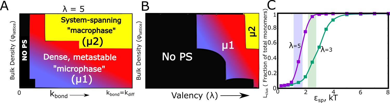
Kinetic Monte Carlo Simulations.

(A) Phase diagram highlighting the different phases (metastable microphase (μ1) or system-spanning macrophase (μ2), and the non-phase separated state (No PS) ) encountered upon increasing $k_{b o n d}$ (between 0 and $k_{d i f f}$ ), and the bulk density of monomers ( $ϕ_{l a t t i c e}$ ) within the box. The assembling particles have a valency ( $λ$ ) of 5 in these simulations. The region shaded yellow represents part of the phase-space where we observe a system-spanning network whereas the bluish-red region represents the metastable micro-phase with a distribution of cluster sizes (see Figure 7—figure supplement 3 for distributions). As we move from the blue to the red regions in this dynamic phase diagram, the size of the single largest cluster increases (also see Figure 7—figure supplement 1). (B) Phase diagram highlighting the different phases encountered upon varying valency and bulk density as the phase parameters. The system-spanning macrophase is only encountered for larger valency particles at higher densities. This phase diagram was computed for $k_{b o n d}$ = $k_{d i f f}$ and $ϵ_{n s}$ of 0.35 kT. (C) The fraction of monomers in the largest cluster as a function of epsilon, for $k_{d i f f}$ = $k_{b o n d}$ and $ϕ_{l a t t i c e}$ = 0.04. The single largest cluster sizes in all sub-panels of this Figure were computed for a simulation time-scale of 2 hr (with the fundamental timsecale of diffusion being set to $k_{d i f f}$ = 1 $s^{- 1}$ ).

Figure 7—source data 1 Compressed zip file containing the source data for kinetic phase diagrams in Figure 7.: https://cdn.elifesciences.org/articles/56159/elife-56159-fig7-data1-v2.zip
Download elife-56159-fig7-data1-v2.zip

Figure 7—figure supplement 1

Download asset Open asset

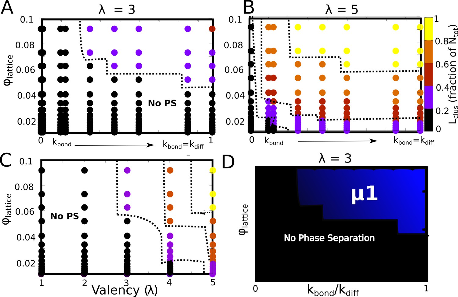
Detailed phase diagrams for (A) and (B) $ϕ$ - $k_{b o n d}$ , (C) $ϕ$ - $λ$ as the phase parameters.

The cluster sizes were computed at the end of a simulation run of 2 hr (actual time), setting the rate of diffusion $k_{d i f f}$ to 1 $s^{- 1}$ . (D) The bonding rate $k_{b o n d}$ was varied to identify the relationship between $k_{b o n d}$ and $k_{d i f f}$ .

Figure 7—figure supplement 2

Download asset Open asset

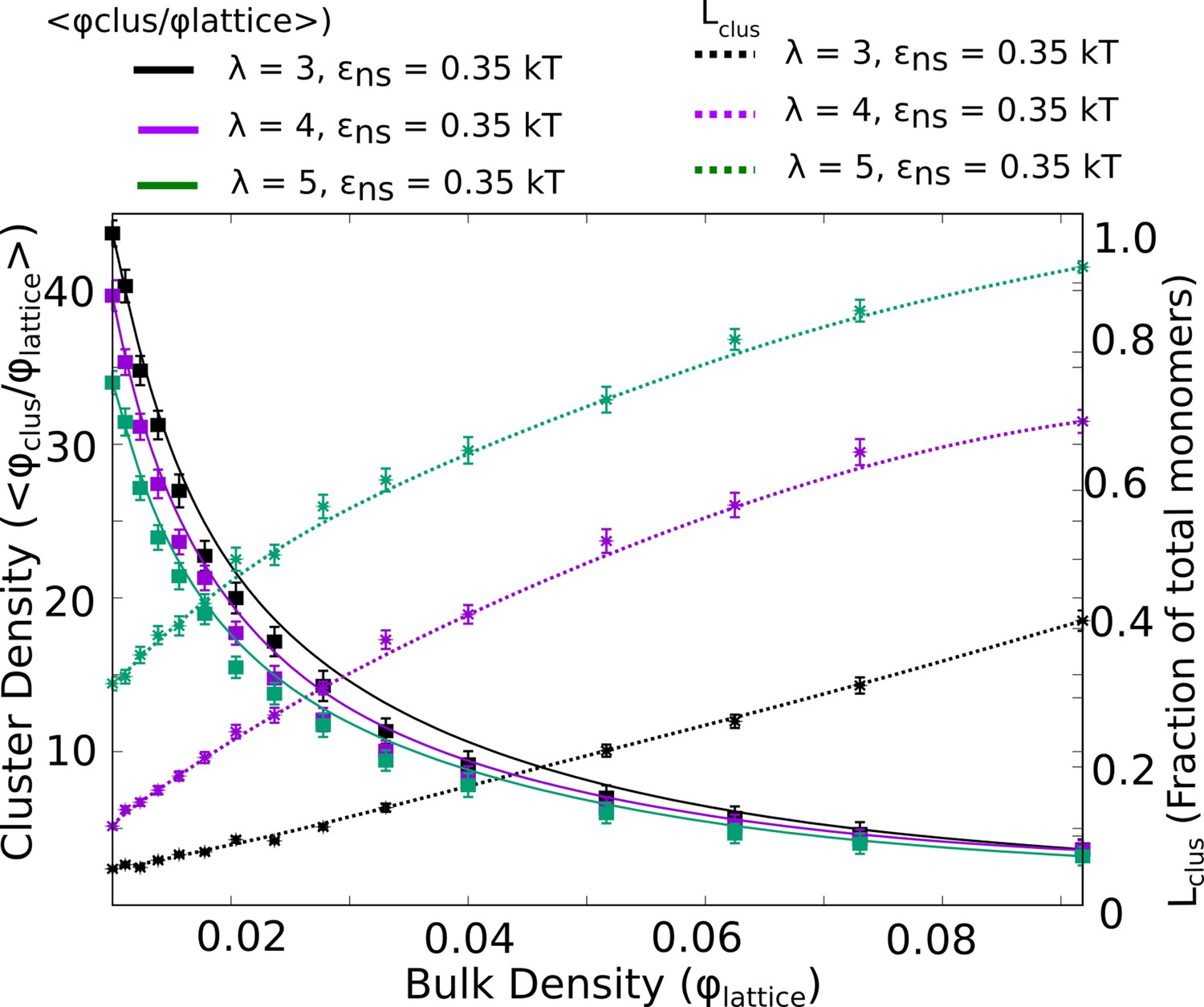
Intra-cluster densities of largest cluster (solid curves) and the corresponding sizes of the single largest cluster (dashed curves) as a function of bulk density, for three different values of $λ$ .

In the regime where cluster sizes approach the total number of monomers, the density of the cluster is at its lowest.

Figure 7—figure supplement 3

Download asset Open asset

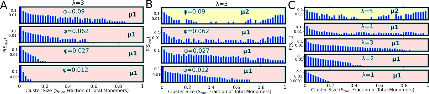
Cluster size distributions for varying densities for λ=3 (A), and λ=5 (B).

(C) Effect of valency on size distributions at a fixed $ϕ_{l a t t i c e}$ of 0.09. These distributions were computed at the end of 100-independent simulation runs of 2 hr (actual time) each. μ1 and μ2, in these figures refer to the macro-phase separated state (with large network-spanning clusters), and the micro-phase separated state (with coexisting clusters of various sizes), respectively. These distributions are representative of the μ1 and μ2 phases shown in the Figure 7 of the main text.

Figure 7—figure supplement 4

Download asset Open asset

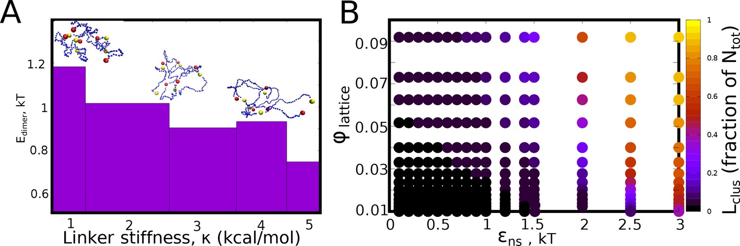
Inter-protein interaction strengths.

(A) The mean pair-wise interaction energy for 100 different dimeric structures (from the LD simulations), for an inter-linker interaction strength of 0.1 kcal/mol, for different values of linker bending rigidity. (B) The $ϵ_{n s}$ - $ϕ$ phase diagram (for $λ$ =0) showing no phase separation for low values of isotropic interaction strength. However, for values of $ϵ_{n s} >$ 1kT, phase separation is observed at the end of the simulation timescale of 2 hr (actual time).

Figure 7—figure supplement 5

Download asset Open asset

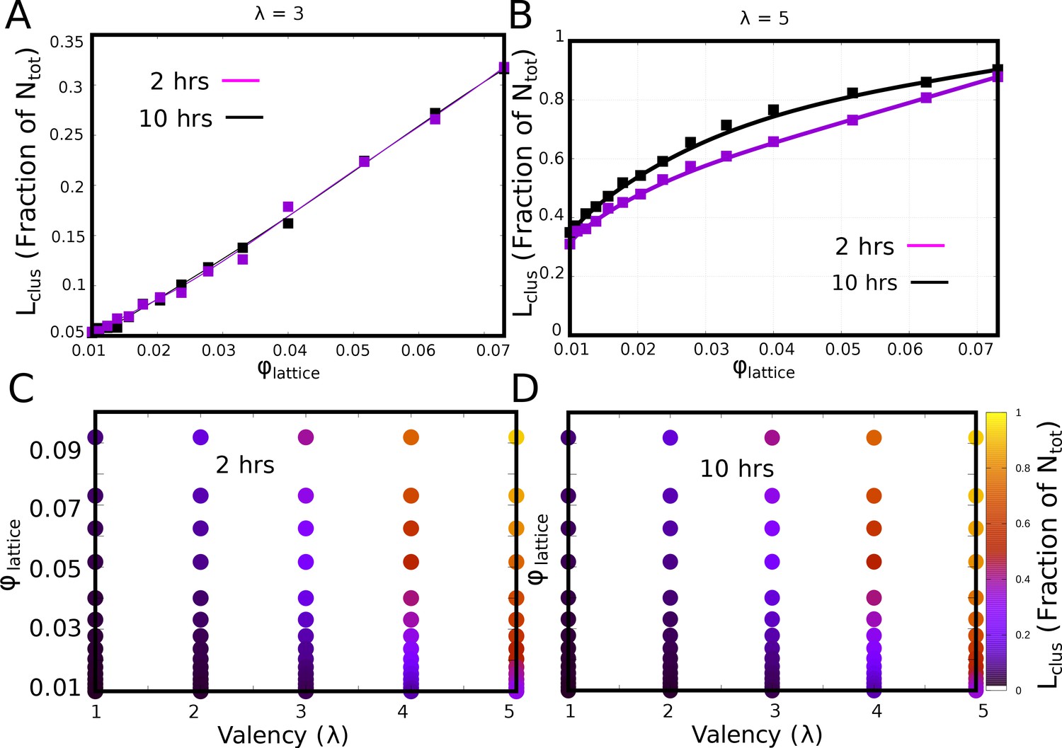
Convergence of phase diagrams.

(A and B) The fraction of monomers in the largest cluster for 2 and 10 hr of actual time, for $λ$ of 3 and 5, respecively. (C and D). The $λ$ - $ϕ$ phase diagram at the end of 2 and 10 hr of simulation time, respectively, showing very little difference.

Figure 7—figure supplement 6

Download asset Open asset

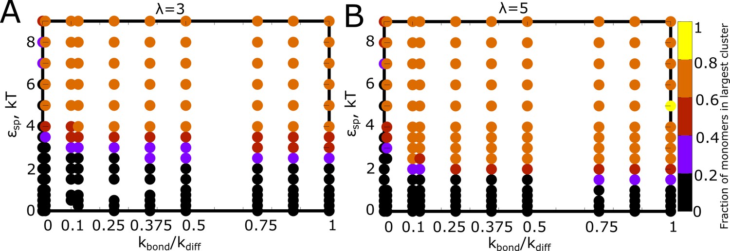
Detailed phase diagrams for (A) and (B) $ϵ_{s p}$ - $k_{b o n d}$ as the phase parameters.

The $ϕ_{l a t t i c e}$ was set to 0.04, an intermediate density identified from the previous phase diagrams with density as a phase parameter. The cluster sizes were computed at the end of a simulation run of 2 hr (actual time), setting the rate of diffusion $k_{d} i f f$ to 1 $s^{- 1}$ .

Figure 8 with 1 supplement

Download asset Open asset

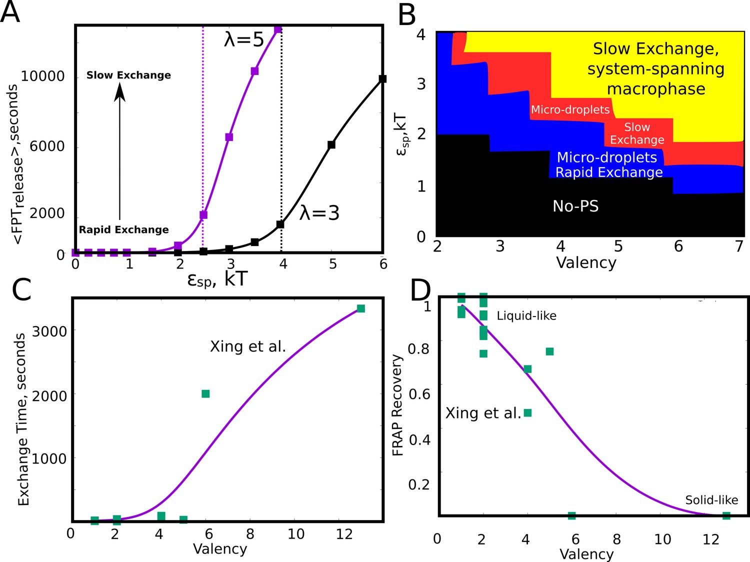
Effect of model parameters on the exchange times between monomers and the aggregates.

The parameter values used in panels A and B are $ϕ_{l a t t i c e}$ =0.04, $k_{b o n d}$ / $k_{d i f f}$ = 1. (A) Mean first passage time for the monomers to go from the buried state (with four neighbors) to the free state (with no neighbors) in response to varying values of specific interaction strength. The two curves show the trends for species with different interaction valencies. The dashed solid lines refer to value of $ϵ_{s p}$ beyond which the largest cluster consumes 50% or more of available monomers. (B) The state of the system, for variation in $ϵ_{s p}$ and $λ$ suggests that the system displays remarkable malleability in dynamicity and size distributions. Weak $ϵ_{s p}$ and a low $λ$ results in no phase separation (shaded black). For higher values of both these parameters, the system can access the single large macro-phasic state (shaded yellow), however with a dramatic slowdown in exchange times. For an intermediate range, the system adopts a metastable microphase separated state, with either slow (shaded red) or fast-exchange (shaded blue) dynamics. (C) The experimentally determined molecular exchange times for molecules of varying interaction valencies. (Xing et al., 2018). (D) The extent of recovery after a photobeaching experiment, for interacting species with varying valencies. The data in panel C) and D) has been obtained from a study by Xing et al., 2018. The solid curves in C and D are added to guide the eye.

Figure 8—source data 1 Compressed zip file containing the source data for kinetic phase diagrams in Figure 8.: https://cdn.elifesciences.org/articles/56159/elife-56159-fig8-data1-v2.zip
Download elife-56159-fig8-data1-v2.zip

Figure 8—figure supplement 1

Download asset Open asset

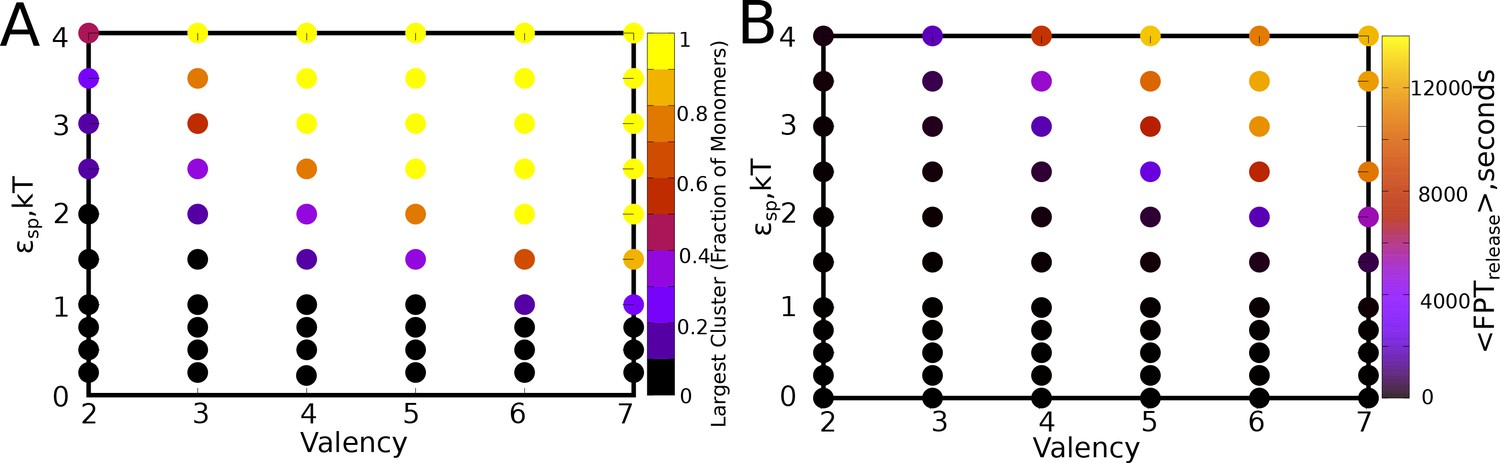
< $L_{c l u s}$ > for varying values of $ϵ_{s p}$ and $λ$ , for a $ϕ_{l a t t i c e}$ of 0.04, and a $k_{b o n d} / k_{d i f f}$ ratio of 1.

(B) Mean first passage times for a particle to exchange between a cluster and the bulk. The parameter values are same as in panel A.

Figure 9 with 1 supplement

Download asset Open asset

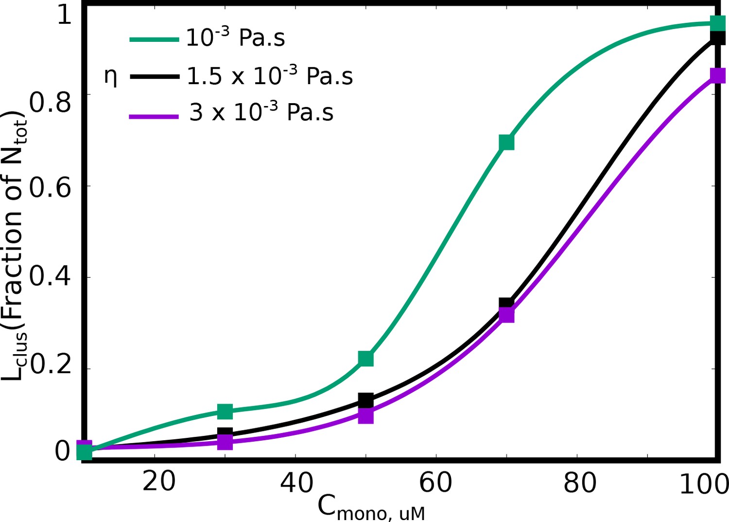
Effect of solvent viscosity.

Langevin Dynamics Simulations. (A and B) Cluster size distributions from Langevin dynamics simulations for different values of solvent viscosity and different free monomer concentrations. The shaded region in the two subpanels (A) and (B) is to highlight that a more viscous solvent results in larger clusters disappearing from the distribution. (C) The size of the single largest cluster as a function of solvent viscosity for a free monomer concentration of 70 μM. (D and E) Monte Carlo Simulations. The size of the single largest cluster as a function of density for varying rates of diffusion, for specific interaction valencies $λ$ =3 (D) and $λ$ = 5 (E).

Figure 9—source data 1 Compressed zip file containing the source data for mean largest cluster sizes (and size distributions) from LD and MC simulations studying the effect of solvent viscosity.: https://cdn.elifesciences.org/articles/56159/elife-56159-fig9-data1-v2.zip
Download elife-56159-fig9-data1-v2.zip

Figure 9—figure supplement 1

Download asset Open asset

$L_{c l u s}$ as a function of free monomer concentrations in LD simulations performed with various solvent viscosities.

Figure 10

Download asset Open asset

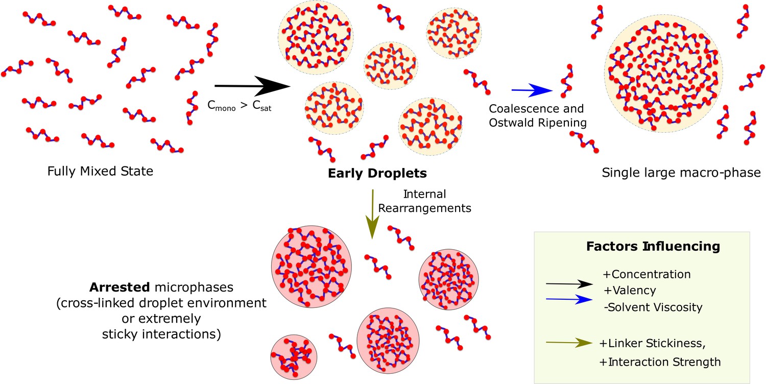
Graphical Summary.

Muli-valent proteins can exist in two Flory-like equilibrium states, the fully mixed solvated state and a single large macro-phase separated state (when free monomer concentration ( $C_{m o n o}$ ) exceeds the critical concentration ( $C_{s a t}$ )). Above the critical concentration, the proteins first phase separate into multiple droplet phases (black arrow) which are long-living, metastable structures. However, the growth of these individual droplets to a single large macro-droplet (blue arrow) through coalescence and Ostwald ripening is unlikely at biologically relevant timescales. The multiple metastable micro-droplets can also age into highly cross-linked structures (green arrow) that saturate interactions within themselves and thus cannot grow further. Extremely stable functional interactions or sticky inter-linker interactions could also result in these arrested microphases.

Tables

Table 1

Important simulation variables and order parameters.

Notation/Terminology	Physical Interpretation	Definition
N_tot	Total number of polymer chains in the system. N_tot = 400 in our simulations.	–
L_clus	Size of the single largest cluster	represented as fraction of N_tot
S_clus	Size of the cluster	represented as fraction of N_tot
C_mono	Concentration of polymer chains in the simulation box	In units of μM
φ	Bulk density of proteins (in their monomeric state) when the individual chains are randomly placed in the simulation box at the start of the simulation.	$ϕ = \frac{N_{t o t}}{(4 / 3) π R_{G}^{3,}} . R_{g}^{'}$ is the the radius of gyration of proteins when they are randomly positioned in simulation box at the start of the simulation.
φ_clus	Intra-cluster density of polymer chains.	$ϕ_{c l u s} = \frac{S_{c l u s}}{(4 / 3) π R_{g}^{3_{c l u s}}} . R_{g}^{c l u s}$ is the radius of gyration of the system of proteins within the cluster.
φ_clus /φ	Normalized intracluster density describing the degree of enrichment of polymer chains within the cluster.	For system-spanning networks, φ_clus/φ→1. For dense clusters, φ_clus/φ >> 1.
ε_ns	Interaction strength for isotropic, non-specific interactions between linker regions. ε_ns in LD simulations is a pairwise interaction strength between individual beads In kMC simulations, ε_ns is the net non-specific interaction strength between two lattice particles.	– .
ε_sp	Strength of attractive interaction between functional domains (specific interactions).	–
φ_lattice	Bulk density of monomers in the 2D-lattice in kMC simulations. This quantity is analogous to the concentration of monomers on the lattice.	φ_lattice = N_tot/L², where L is the size of the 2D square-lattice.
λ	Valency of the polymer chain, that is the number of adhesive functional domains per interacting polymer chain.	–
Κ	Bending stiffness of the linker regions in LD simulations. A higher value of K is used to model stiffer linkers that prefer a more open configuration.	Κ = 2 kcal/mol, in LD simulations with flexible linkers.
η	The viscosity of the medium in LD simulations	η = 10⁻³Pa.s in LD simulations, unless mentioned otherwise.
k_diff	Diffusion rate of free monomers in the 2D-lattice kMC simulations.	–
k_bond	Rate of formation of specific interactions between neighboring particles in 2D-lattice kMC simulations.	–

Additional files

Source code 1 Langevin Dynamics Simulation LAMMPS Script. Langevin dynamics simulation script.: https://cdn.elifesciences.org/articles/56159/elife-56159-code1-v2.zip
Download elife-56159-code1-v2.zip
Transparent reporting form: https://cdn.elifesciences.org/articles/56159/elife-56159-transrepform-v2.docx
Download elife-56159-transrepform-v2.docx

Download links

A two-part list of links to download the article, or parts of the article, in various formats.

Downloads (link to download the article as PDF)

Open citations (links to open the citations from this article in various online reference manager services)

Mendeley

Cite this article (links to download the citations from this article in formats compatible with various reference manager tools)

Srivastav Ranganathan
Eugene I Shakhnovich

(2020)

Dynamic metastable long-living droplets formed by sticker-spacer proteins

eLife 9:e56159.

https://doi.org/10.7554/eLife.56159

Share this article

Cite this article

Model.

Cluster Sizes in Langevin Dynamics simulations.

Figure 2—source data 1

Cluster Sizes in Langevin Dynamics simulations.

Tracking cluster formation at early timescales.

Figure 3—source data 1

The size of the largest cluster, for different values of bond formation probability, Pf⁢o⁢r⁢m.

Factors influencing the key timescales.

Figure 4—source data 1

Linkers as modulators of self-assembly propensity.

Figure 5—source data 1

Fraction of valencies utilized as a function of increasing inter-linker interaction strength, for (A) 10 μM and (B) 50 μM free monomer concentration.

The probability of finding clusters with varying densities (normalized by the bulk densities) for different values of inter-linker interactions.

Comparision between the size distributions of the largest cluster, for flexible (κ=2 kcal/mol) versus stiff (κ=5 kcal/mol) linker regions.

A schematic figure detailing the different rates in our phenomenological kinetic model simulated using the Gillespie algorithm.

Kinetic Monte Carlo Simulations.

Figure 7—source data 1

Detailed phase diagrams for (A) and (B) ϕ-kb⁢o⁢n⁢d, (C) ϕ-λ as the phase parameters.

Intra-cluster densities of largest cluster (solid curves) and the corresponding sizes of the single largest cluster (dashed curves) as a function of bulk density, for three different values of λ.

Cluster size distributions for varying densities for λ=3 (A), and λ=5 (B).

Inter-protein interaction strengths.

Convergence of phase diagrams.

Detailed phase diagrams for (A) and (B) ϵs⁢p-kb⁢o⁢n⁢d as the phase parameters.

Effect of model parameters on the exchange times between monomers and the aggregates.

Figure 8—source data 1

<Lc⁢l⁢u⁢s> for varying values of ϵs⁢p and λ, for a ϕl⁢a⁢t⁢t⁢i⁢c⁢e of 0.04, and a kbond/kdiff ratio of 1.

Effect of solvent viscosity.

Figure 9—source data 1

Lc⁢l⁢u⁢s as a function of free monomer concentrations in LD simulations performed with various solvent viscosities.

Graphical Summary.

Important simulation variables and order parameters.

Source code 1

Transparent reporting form

Downloads (link to download the article as PDF)

Open citations (links to open the citations from this article in various online reference manager services)

Cite this article (links to download the citations from this article in formats compatible with various reference manager tools)

The size of the largest cluster, for different values of bond formation probability, $P_{f o r m}$ .

Comparision between the size distributions of the largest cluster, for flexible ( $κ$ =2 kcal/mol) versus stiff ( $κ$ =5 kcal/mol) linker regions.

Detailed phase diagrams for (A) and (B) $ϕ$ - $k_{b o n d}$ , (C) $ϕ$ - $λ$ as the phase parameters.

Intra-cluster densities of largest cluster (solid curves) and the corresponding sizes of the single largest cluster (dashed curves) as a function of bulk density, for three different values of $λ$ .

Detailed phase diagrams for (A) and (B) $ϵ_{s p}$ - $k_{b o n d}$ as the phase parameters.

< $L_{c l u s}$ > for varying values of $ϵ_{s p}$ and $λ$ , for a $ϕ_{l a t t i c e}$ of 0.04, and a $k_{b o n d} / k_{d i f f}$ ratio of 1.

$L_{c l u s}$ as a function of free monomer concentrations in LD simulations performed with various solvent viscosities.