Training deep neural density estimators to identify mechanistic models of neural dynamics
Figures
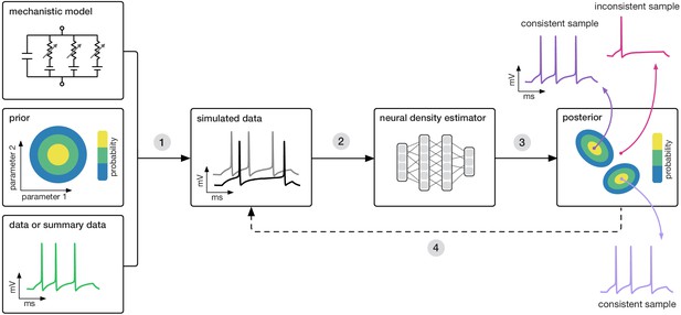
Goal: algorithmically identify mechanistic models which are consistent with data.
Our algorithm (SNPE) takes three inputs: a candidate mechanistic model, prior knowledge or constraints on model parameters, and data (or summary statistics). SNPE proceeds by (1) sampling parameters from the prior and simulating synthetic datasets from these parameters, and (2) using a deep density estimation neural network to learn the (probabilistic) association between data (or data features) and underlying parameters, that is to learn statistical inference from simulated data. (3) This density estimation network is then applied to empirical data to derive the full space of parameters consistent with the data and the prior, that is, the posterior distribution. High posterior probability is assigned to parameters which are consistent with both the data and the prior, low probability to inconsistent parameters. (4) If needed, an initial estimate of the posterior can be used to adaptively guide further simulations to produce data-consistent results.
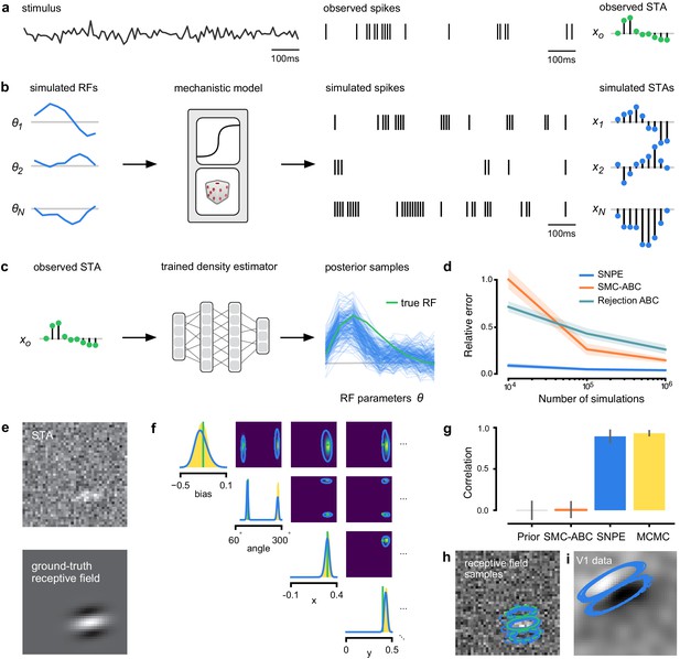
Estimating receptive fields in linear-nonlinear models of single neurons with statistical inference.
(a) Schematic of a time-varying stimulus, associated observed spike train and resulting spike-triggered average (STA) (b) Sequential Neural Posterior Estimation (SNPE) proceeds by first randomly generating simulated receptive fields θ, and using the mechanistic model (here an LN model) to generate simulated spike trains and simulated STAs. (c) These simulated STAs and receptive fields are then used to train a deep neural density estimator to identify the distribution of receptive fields consistent with a given observed STA . (d) Relative error in posterior estimation of SNPE and alternative methods (mean and 95% CI; 0 corresponds to perfect estimation, one to prior-level, details in Materials and methods). (e) Example of spatial receptive field. We simulated responses and an STA of an LN-model with oriented receptive field. (f) We used SNPE to recover the distribution of receptive-field parameters. Univariate and pairwise marginals for four parameters of the spatial filter (MCMC, yellow histograms; SNPE, blue lines; ground truth, green; full posterior in Appendix 1—figure 4). Non-identifiabilities of the Gabor parameterization lead to multimodal posteriors. (g) Average correlation (± SD) between ground-truth receptive field and receptive field samples from posteriors inferred with SMC-ABC, SNPE, and MCMC (which provides an upper bound given the inherent stochasticity of the data). (h) Posterior samples from SNPE posterior (SNPE, blue) compared to ground-truth receptive field (green; see panel (e)), overlaid on STA. (i) Posterior samples for V1 data; full posterior in Appendix 1—figure 6.
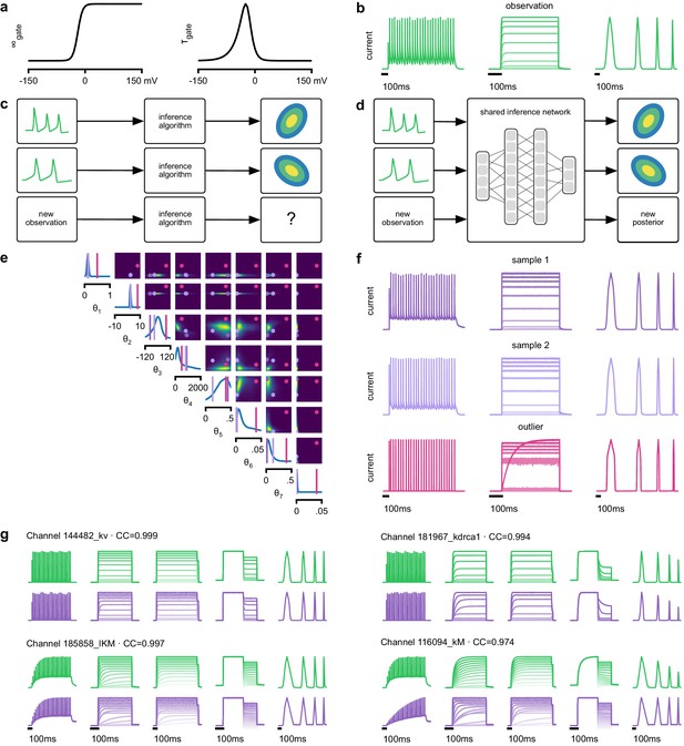
Inference on a database of ion-channel models.
(a) We perform inference over the parameters of non-inactivating potassium channel models. Channel kinetics are described by steady-state activation curves, , and time-constant curves, . (b) Observation generated from a channel model from ICG database: normalized current responses to three (out of five) voltage-clamp protocols (action potentials, activation, and ramping). Details in Podlaski et al., 2017. (c) Classical approach to parameter identification: inference is optimized on each datum separately, requiring new computations for each new datum. (d) Amortized inference: an inference network is learned which can be applied to multiple data, enabling rapid inference on new data. (e) Posterior distribution over eight model parameters, to . Ground truth parameters in green, high-probability parameters in purple, low-probability parameters in magenta. (f) Traces obtained by sampling from the posterior in (e). Purple: traces sampled from posterior, that is, with high posterior probability. Magenta: trace from parameters with low probability. (g) Observations (green) and traces generated by posterior samples (purple) for four models from the database.
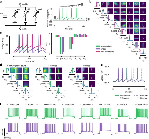
Inference for single compartment Hodgkin–Huxley model.
(a) Circuit diagram describing the Hodgkin–Huxley model (left), and simulated voltage-trace given a current input (right). Three out of 7 voltage features are depicted: (1) number of spikes, (2) mean resting potential, and (3) standard deviation of the pre-stimulus resting potential. (b) Inferred posterior for 8 parameters given seven voltage features. Ground truth parameters in green, high-probability parameters in purple, low-probability parameters in magenta. (c) Traces (left) and associated features f (right) for the desired output (observation), the mode of the inferred posterior, and a sample with low posterior probability. The voltage features are: number of spikes , mean resting potential , standard deviation of the resting potential , and the first four voltage moments, mean , standard deviation , skewness and kurtosis . Each value plotted is the mean feature ± standard deviation across 100 simulations with the same parameter set. Each feature is normalized by , the standard deviation of the respective feature of simulations sampled from the prior. (d) Partial view of the inferred posteriors (4 out of 8 parameters) given 1, 4 and 7 features (full posteriors over eight parameters in Appendix 1—figure 8). (e) Traces for posterior modes given 1, 4 and 7 features. Increasing the number of features leads to posterior traces that are closer to the observed data. (f) Observations from Allen Cell Types Database (green) and corresponding mode samples (purple). Posteriors in Appendix 1—figure 9.
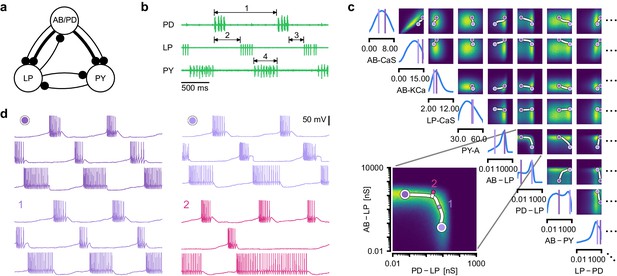
Identifying network models underlying an experimentally observed pyloric rhythm in the crustacean stomatogastric ganglion.
(a) Simplified circuit diagram of the pyloric network from the stomatogastric ganglion. Thin connections are fast glutamatergic, thick connections are slow cholinergic. (b) Extracellular recordings from nerves of pyloric motor neurons of the crab Cancer borealis (Haddad and Marder, 2018). Numbers indicate some of the used summary features, namely cycle period (1), phase delays (2), phase gaps (3), and burst durations (4) (see Materials and methods for details). (c) Posterior over 24 membrane and seven synaptic conductances given the experimental observation shown in panel b (eight parameters shown, full posterior in Appendix 1—figure 11). Two high-probability parameter sets in purple. Inset: magnified marginal posterior for the synaptic strengths AB to LP neuron vs. PD to LP neuron. (d) Identifying directions of sloppiness and stiffness. Two samples from the posterior both show similar network activity as the experimental observation (top left and top right), but have very different parameters (purple dots in panel c). Along the high-probability path between these samples, network activity is preserved (trace 1). When perturbing the parameters orthogonally off the path, network activity changes abruptly and becomes non-pyloric (trace 2).
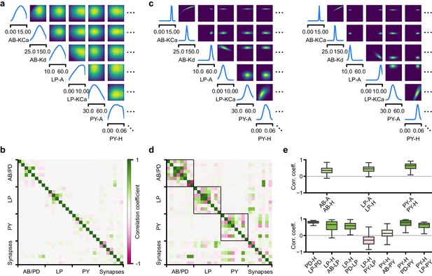
Predicting compensation mechanisms in the stomatogastric ganglion.
(a) Inferred posterior. We show a subset of parameters which are weakly constrained (full posterior in Appendix 1—figure 11). Pyloric activity can emerge from a wide range of maximal membrane conductances, as the 1D and 2D posterior marginals cover almost the entire extent of the prior. (b) Correlation matrix, based on the samples shown in panel (a). Almost all correlations are weak. Ordering of membrane and synaptic conductances as in Appendix 1—figure 11. (c) Conditional distributions given a particular circuit configuration: for the plots on the diagonal, we keep all but one parameter fixed. For plots above the diagonal, we keep all but two parameters fixed. The remaining parameter(s) are narrowly tuned; tuning across parameters is often highly correlated. When conditioning on a different parameter setting (right plot), the conditional posteriors change, but correlations are often maintained. (d) Conditional correlation matrix, averaged over 500 conditional distributions like the ones shown in panel (c). Black squares highlight parameter-pairs within the same model neuron. (e) Consistency with experimental observations. Top: maximal conductance of the fast transient potassium current and the maximal conductance of the hyperpolarization current are positively correlated for all three neurons. This has also been experimentally observed in the PD and the LP neuron (MacLean et al., 2005). Bottom: the maximal conductance of the hyperpolarization current of the postsynaptic neuron can compensate the strength of the synaptic input, as experimentally observed in the PD and the LP neuron (Grashow et al., 2010; Marder, 2011). The boxplots indicate the maximum, 75% quantile, median, 25% quantile, and minimum across 500 conditional correlations for different parameter pairs. Face color indicates mean correlation using the colorbar shown in panel (b).

Comparison between SNPE-estimated posterior and reference posterior (obtained via MCMC) on LN model.
(a) Posterior mean ± one standard deviation of temporal filter (receptive field) from SNPE posterior (SNPE, blue) and reference posterior (MCMC, yellow). (b) Full covariance matrices from SNPE posterior (left) and reference (MCMC, right).
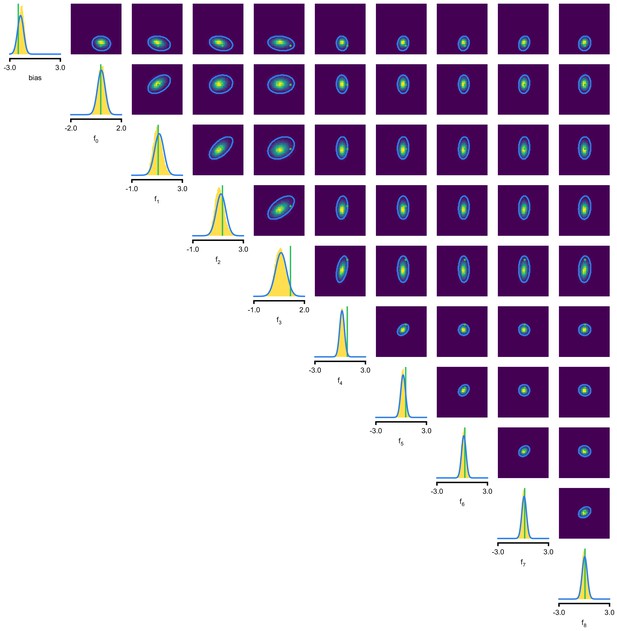
Full posterior for LN model.
In green, ground-truth parameters. Marginals (blue lines) and 2D marginals for SNPE (contour lines correspond to 95% of the mass) and MCMC (yellow histograms).
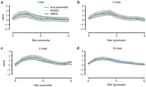
LN model with additional data.
With additional data, posterior samples cluster more tightly around the true filter. From left to right and top to bottom, SNPE (blue) and MCMC (yellow, for reference) are applied to observations with more independent Bernoulli trials, leading to progressively tighter posteriors and posterior samples closer to the true filter (which is the same across panels). Mean ± one standard deviation is shown. Note that SNPE closely agrees with the MCMC reference solution in all cases (a-d).
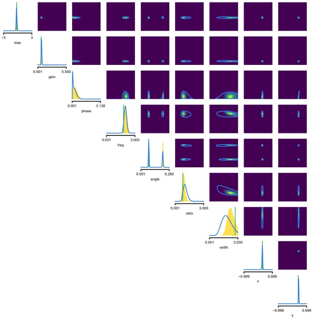
Full posterior for Gabor GLM receptive field model.
SNPE posterior estimate (blue lines) compared to reference posterior (MCMC, histograms). Ground-truth parameters used to simulate the data in green. We depict the distributions over the original receptive field parameters, whereas we estimate the posterior as a Gaussian mixture over transformed parameters, see Materials and methods for details. We find that a (back-transformed) Gaussian mixture with four components approximates the posterior well in this case.
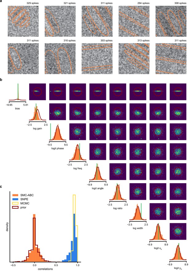
SMC-ABC posterior estimate for Gabor GLM receptive field model.
(a) Spike-triggered averages (STAs) and spike counts with closest distance to the observed data out of 10000 simulations with parameters sampled from the prior. Spike counts are comparable to the observed data (299 spikes), but receptive fields (contours) are not well constrained. (b) Results for SMC-ABC with a total of 106 simulations. Histograms of 1000 particles (orange) returned in the final iteration of SMC-ABC, compared to prior (red contour lines) and ground-truth parameters (green). Distributions over (log-/logit-)transformed parameters, axis limits scaled to mean ± 3 standard deviations of the prior. (c) Correlations between ground-truth receptive field and receptive fields sampled from SMC-ABC posterior (orange), SNPE posterior (blue), reference MCMC posterior (yellow) and prior (red). The SNPE-estimated receptive fields are almost as good as those of the reference posterior, the SMC-ABC estimated ones no better than the prior.
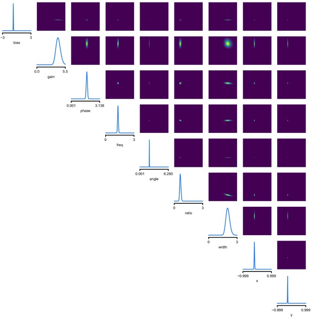
Full posterior for Gabor LN receptive field model on V1 recordings.
We depict the distributions over the receptive field parameters, derived from the Gaussian mixture over transformed-parameters (see Materials and methods for details).
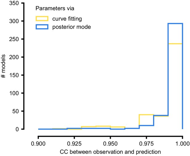
Summary results on 350 ICG channel models, and comparison with direct fits.
We generate predictions either with the posterior mode (blue) or with parameters obtained by directly fitting steady-state activation and time-constant curves (yellow). We calculate the correlation coefficient (CC) between observation and prediction. The distribution of CCs is similar for both approaches.
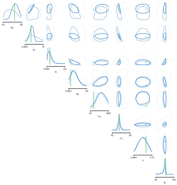
Full posteriors for Hodgkin-Huxley model for 1, 4, and 7 features.
Images show the pairwise marginals for 7 features. Each contour line corresponds to 68% density mass for a different inferred posterior. Light blue corresponds to 1 feature and dark blue to 7 features. Ground truth parameters in green.
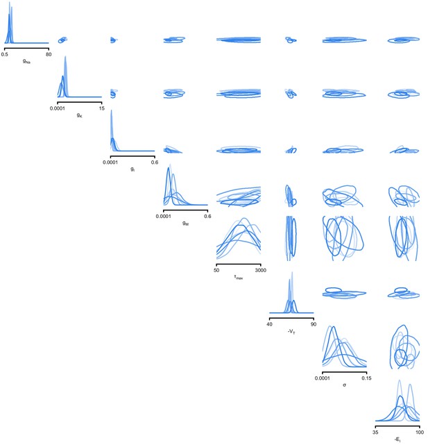
Full posteriors for Hodgkin-Huxley model on 8 different recordings from Allen Cell Type Database.
Images show the pairwise marginals for 7 features. Each contour line corresponds to 68% density mass for a different inferred posterior.
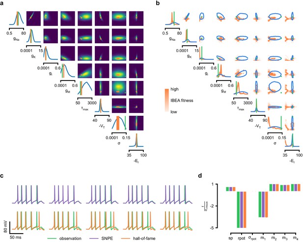
Comparison between SNPE posterior and IBEA samples for Hodgkin-Huxley model with 8 parameters and 7 features.
(a) Full SNPE posterior distribution. Ground truth parameters in green and IBEA 10 parameters with highest fitness (‘hall-of-fame’) in orange. (b) Blue contour line corresponds to 68% density mass for SNPE posterior. Light orange corresponds to IBEA sampled parameters with lowest IBEA fitness and dark orange to IBEA sampled parameters with highest IBEA fitness. This plot shows that, in general, SNPE and IBEA can return very different answers– this is not surprising, as both algorithms have different objectives, but this highlights that genetic algorithms do not in general perform statistical inference. (c) Traces for samples with high probability under SNPE posterior (purple), and for samples with high fitness under IBEA objective (hall-of-fame; orange traces). (d) Features for the desired output (observation), the mode of the inferred posterior (purple) and the best sample under IBEA objective (orange). Each voltage feature is normalized by , the standard deviation of the respective feature of simulations sampled from the prior.
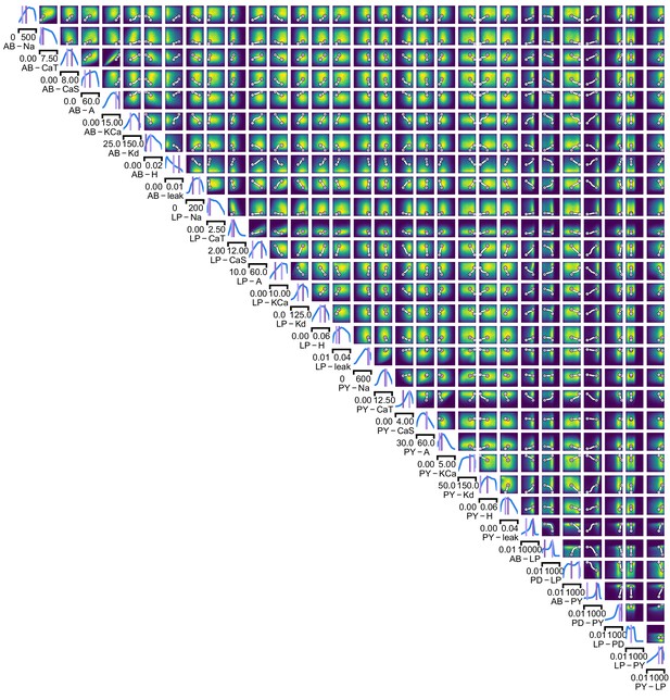
Full posterior for the stomatogastric ganglion over 24 membrane and 7 synaptic conductances.
The first 24 dimensions depict membrane conductances (top left), the last 7 depict synaptic conductances (bottom right). All synaptic conductances are logarithmically spaced. Between two samples from the posterior with high posterior probability (purple dots), there is a path of high posterior probability (white).
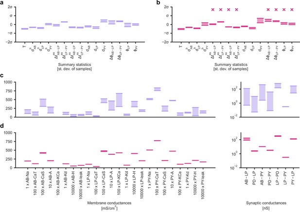
Identifying directions of sloppiness and stiffness in the pyloric network of the crustacean stomatogastric ganglion.
(a) Minimal and maximal values of all summary statistics along the path lying in regions of high posterior probability, sampled at 20 evenly spaced points. Summary statistics change only little. The summary statistics are z-scored with the mean and standard deviation of 170,000 bursting samples in the created dataset. (b) Summary statistics sampled at 20 evenly spaced points along the orthogonal path. The summary statistics show stronger changes than in panel a and, in particular, often could not be defined because neurons bursted irregularly, as indicated by an ‘x’ above barplots. (c) Minimal and maximal values of the circuit parameters along the path lying in regions of high posterior probability. Both membrane conductances (left) and synaptic conductances (right) vary over large ranges. Axes as in panel (d). (d) Circuit parameters along the orthogonal path. The difference between the minimal and maximal value is much smaller than in panel (c).
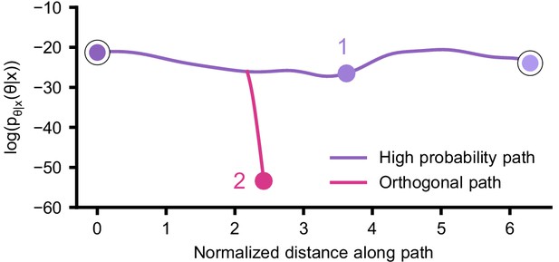
Posterior probability along high probability and orthogonal path.
Along the path that was optimized to lie in regions of high posterior probability (purple), the posterior probability remains relatively constant. Along the orthogonal path (pink), optimized to quickly reduce posterior probability, the probability quickly drops. The start and end points as well as the points labeled 1 and 2 correspond to the points shown in Figure 5c.
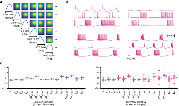
Evaluating circuit configurations in which parameters have been sampled independently.
(a) Factorized posterior, that is, posterior obtained by sampling each parameter independently from the associated marginals. Many of the pairwise marginals look similar to the full posterior shown in Appendix 1—figure 11, as the posterior correlations are low. (b) Samples from the factorized posterior– only a minority of these samples produce pyloric activity, highlighting the significance of the posterior correlations between parameters. (c) Left: summary features for 500 samples from the posterior. Boxplot for samples where all summary features are well-defined (80% of all samples). Right: summary features for 500 samples from the factorized posterior. Only 23% of these samples have well-defined summary features. The summary features from the factorized posterior have higher variation than the posterior ones. Summary features are z-scored using the mean and standard deviation of all samples in our training dataset obtained from prior samples. The boxplots indicate the maximum, 75% quantile, median, 25% quantile, and minimum. The green ‘x’ indicates the value of the experimental data (the observation, shown in Figure 5b).


