Paranoia as a deficit in non-social belief updating
- Interdepartmental Neuroscience Program, Yale School of Medicine, United States
- Yale MD-PhD Program, Yale School of Medicine, United States
- Princeton Neuroscience Institute, Princeton University, United States
- Department of Psychiatry, Connecticut Mental Health Center, Yale University, United States
- Scuola Internazionale Superiore di Studi Avanzati (SISSA), Italy
- Translational Neuromodeling Unit (TNU), Institute for Biomedical Engineering, University of Zurich and ETH Zurich, Switzerland
Figures
Figure 1
Probabilistic reversal learning task.
(a) Human paradigm: participants choose between three decks of cards with different colored backs (Blue, Red, and Green) with different, unknown probabilities of reward and loss. (b) Reward contingency schedule for in laboratory experiment (Reward probabilities associated with the different colored decks, Blue, Red, Green, across trials and blocks). On trial 81, the probability context shifted from 90%, 50%, and 10% (dark grey) to 80%, 40%, and 20% without warning (light grey). (c), Reward contingency schedules for online experiment. (d) Rat paradigm: subjects choose between three noseports (Blue, Red, Green, for illustrative puposes) with different probabilities of sucrose pellet reward. (e) Reward contingency schedule for rat experiment (Groman et al., 2018). Performance dependent reversals occur after a certain number of choices of the high reward deck. Performance independent reversals occur regardless of participant behavior.
Figure 2
Hierarchical Gaussian Filter (HGF) model parameters.
(a) 3-level HGF perceptual model (blue) with a softmax decision model (green). Level 1 (x1): trial-by-trial perception of win or loss feedback. Level 2 (x2): stimulus-outcome associations (i.e., deck values). Level 3 (x3): perception of the overall reward contingency context. The impact of phasic volatility upon x2 is captured by κ (i.e., coupling). Tonic volatility modulates x3 and x2 via ω3 and ω2, respectively. μ30 is the initial value of the third level volatility belief. (b) HGF model parameter estimates from each of our three studies (in laboratory, online, rat - columns), ω3, μ30, κ, and ω2, displayed hierarchically, in rows, in parallel with the position of the particular parameter in the model depiction in a). Parameters replicate across high paranoia groups in the in-laboratory experiment (n = 21 low paranoia [gray], 11 high paranoia [orange]; dark bars are initial task blocks, lighter bars follow the contingency transition); the analogous online task (version 3, n = 56 low paranoia [gray], 16 high paranoia [orange]; dark bars are initial task blocks, lighter bars follow the contingency transition); and rats exposed to chronic, escalating saline or methamphetamine (n = 10 per group, Pre-Rx [dark gray]; Post-Rx, n = 10 saline [light gray], seven methamphetamine [orange]). Center lines depict medians; box limits indicate the 25th and 75th percentiles; whiskers extend 1.5 times the interquartile range from the 25th and 75th percentiles, outliers are represented by dots; crosses represent sample means; data points are plotted as open circles. *p≤0.05, **p≤0.01, ***p≤0.001.
Figure 3
Paranoia effects across task versions.
(a) Estimated model parameters derived from participant choices in response to the tasks. Low paranoia is shown in gray, high paranoia is shown in orange. μ30, κ, and ω2 are shown in separate panels (top, middle, and bottom panels, respectively; y-axes). X-axes depict each separate online task version from Experiment 2 (version 1: Easy-Easy, version 2: Hard-Hard, version 3: Easy-Hard, version 4: Hard-Easy). (b) Behavior. Win-switch rate (top): paranoid participants switched between decks more frequently after positive feedback. Rates are collapsed across all task versions and blocks (paranoia group effect; n = 234 low paranoia [gray], 73 high paranoia [orange]). U-value (bottom): a measure of choice stochasticity, calculated for low (gray) and high (orange) paranoia participants and collapsed across task blocks. U-values are shown separately for each online task version (1 through 4, as in part a). In versions 3 and 4 only (the versions containing unsignaled contingency transitions), paranoid participants showed higher U-values, suggesting increasingly stochastic switching rather than perseverative returns to a previously rewarding option. Center lines show the medians; box limits indicate the 25th and 75th percentiles; whiskers extend 1.5 times the interquartile range from the 25th and 75th percentiles, outliers are represented by dots; crosses represent sample means; data points are plotted as open circles. P-values correspond to estimated marginal means post-hoc comparisons: *p≤0.05, **p≤0.01, ***p≤0.001.
Figure 4
Correlations between κ and symptoms, with and without paranoia scores of zero.
Paranoia (SCID-II, top), depression (BDI, middle), and anxiety (BAI, bottom). (a) Among all 72 subjects from online version 3, κ correlates with paranoia (r = 0.30, p=0.011, top) and depression (r = 0.250, p=0.034, middle), but not anxiety (r = 0.210, p=0.077, bottom). (b) Among participants who endorse at least one paranoia item (SCID-II paranoia >0, n = 39), κ correlates with paranoia (r = 0.588, p=8.1E-5, top), depression (r = 0.427, p=0.007, middle), and anxiety (r = 0.367, p=0.021, bottom). All correlations are two-tailed.
Figure 5
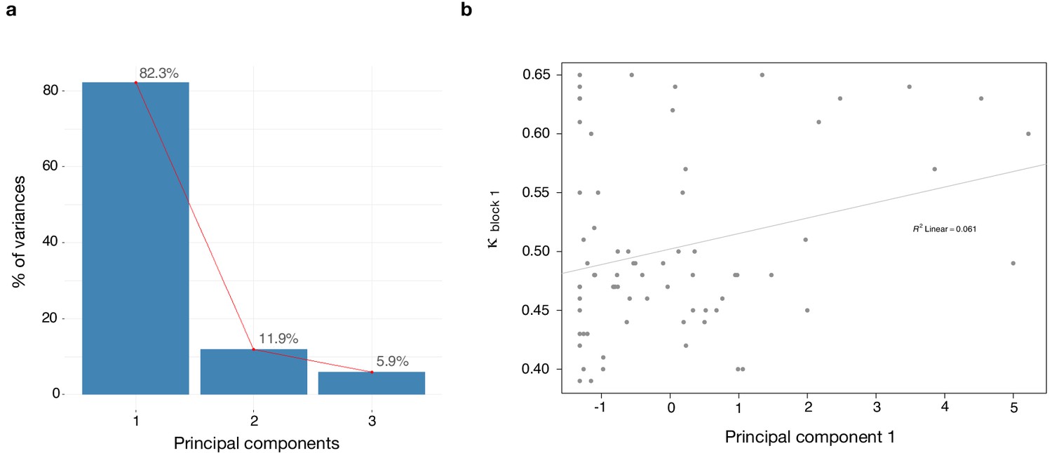
Dimensionality reduction analysis.
Principal component analysis (PCA) was performed on behavioral data to explain the relationship between κ and the rating scales - paranoia (SCID), depression (BDI) and anxiety (BAI). (a) Scree plot of PCA illustrates percent of variance for each component explained by SCID, BDI and BAI. (b) Principal component 1 (PC1) plotted against κ values. κ correlates with PC1 (r = 0.272, p=0.021).
Figure 6
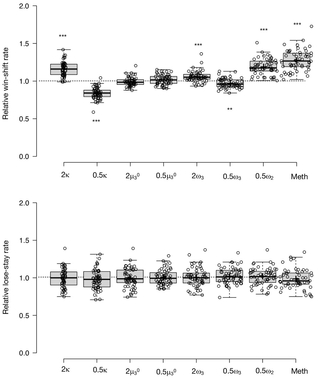
Parameter effects on simulated task performance.
We simulated behavior from low paranoia participants (online Version 3, n = 54) to evaluate the effects of κ,μ30, ω2, and ω3 on win-shift and lose-stay rates. Estimated perceptual parameters were averaged across subjects to create a single set of baseline parameters. Additional parameter sets were created by doubling or halving one parameter at a time (e.g., 2 κ or 0.5 κ), while the others were held constant (n.b., 2 ω2 violated model assumptions and was excluded from analysis). We also included the average parameter values of rats exposed to methamphetamine (Meth). Ten simulations were run per subject for each condition (i.e., parameter set). Win-shift and lose-stay rates were calculated, then averaged across simulations and subjects. Rates from each condition were divided by the baseline condition rate to generate relative win-shift and lose-stay rates. We compared relative rates for each condition to the baseline (relative rate of 1, depicted as the dotted line; paired t-tests, Bonferroni-corrected p-values). Of note, baseline parameters were positive for κ and ω2, and negative for μ30 and ω3. Consequently, the doubled (2x) condition makes μ30 and ω3 more negative (lower). (n = 54). Box-plots: center lines show the medians; box limits indicate the 25th and 75th percentiles; whiskers extend 1.5 times the interquartile range from the 25th and 75th percentiles, outliers are represented by dots; crosses represent sample means; data points are plotted as open circles; *p≤0.05, **p≤0.01, ***p≤0.001.
Figure 7
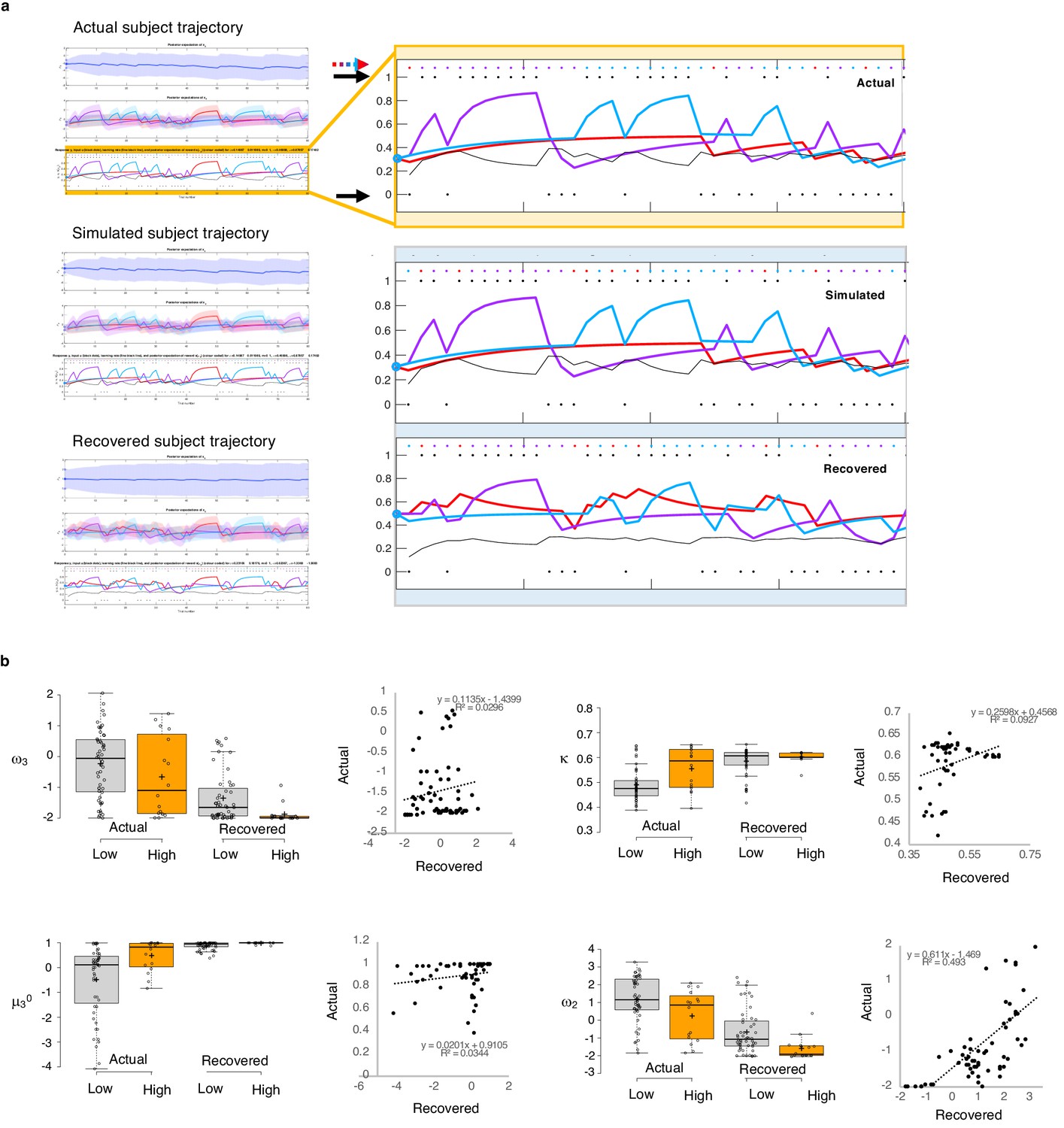
Parameter recovery.
(a) Actual subject trajectory: this is an example choice trajectory from one participant (top). The layers correspond to the three layers of belief in the HGF model (depicted in Figure 2a). Focusing on the low-level beliefs (yellow box): The purple line represents the subject’s estimated first-level belief about the value of choosing deck 1; blue, their belief about the value of choosing deck 2; and red, their belief about the value of choosing deck 3. Simulated subject trajectory represents the estimated beliefs from choices simulated from estimated perceptual parameters from that participant (middle), and Recovered subject trajectory represents what happens when we re-estimate beliefs from the simulated choices (bottom). Crucially, Simulated trajectories closely align with real trajectories (the increases and decreased in estimated beliefs about the values of each deck [purple, blue, red lines] align with each other across actual, simulated and recovered trajectories), although trial-by-trial choices (colored dots and arrow) occasionally differ. Outcomes (1 or 0; black dots and arrows) remain the same. (b) Actual versus Recovered: these data represent the belief parameters estimated from the participant’s responses (Actual) compared to those estimated from the choices simulated with the participant’s perceptual parameters (Recovered). Actual and Recovered values significantly correlate for ω2 (r = 0.702, p=2.52E-11) and κ (r = 0.305, p=0.011) but not ω3 (r = 0.172, p=0.16) or µ30 (r = 0.186, p=0.13). Box plots: gray indicates low paranoia, orange designates high paranoia; center lines depict medians; box limits indicate the 25th and 75th percentiles; whiskers extend 1.5 times the interquartile range from the 25th and 75th percentiles, outliers are represented by dots; crosses represent sample means; data points are plotted as open circles. Online version three dataset.
Figure 8

Behavioral data and simulations.
(a) Plots of in laboratory and online behavioral metrics. Win-switch rate (switching after positive feedback), U-value (behavioral stochasticity) and Lose-stay rate (perseverating after a loss). Low paranoia participants are shown in gray, High paranoia in orange. Win-switch rates and U-values are collapsed across blocks. For Lose-stay rates, darker colors are block one data and lighter colors are block two data. Behavioral switching patterns replicate across in laboratory and online version three experiments. Perseveration after negative feedback (lose-stay behavior) did not significantly differ between paranoia groups or task block. (b) Simulated data generated from HGF perceptual parameters (version 3). Win-switch rate, U-value and Lose-stay rate of the simulated data are depicted. The model simulated data replicate the win-switch and U-value behavioral differences between high and low paranoia participants presented in panel a. Like the real participants, there was no difference in lose-stay rates in the simulated data. Center lines show the medians; box limits indicate the 25th and 75th percentiles; whiskers extend 1.5 times the interquartile range from the 25th and 75th percentiles, outliers are represented by dots; crosses represent sample means; data points are plotted as open circles.*p≤0.05, **p≤0.01, ***p≤0.001. Plots of participant behavioral metrics (a) are presented side by side with simulated data (b).
Figure 9
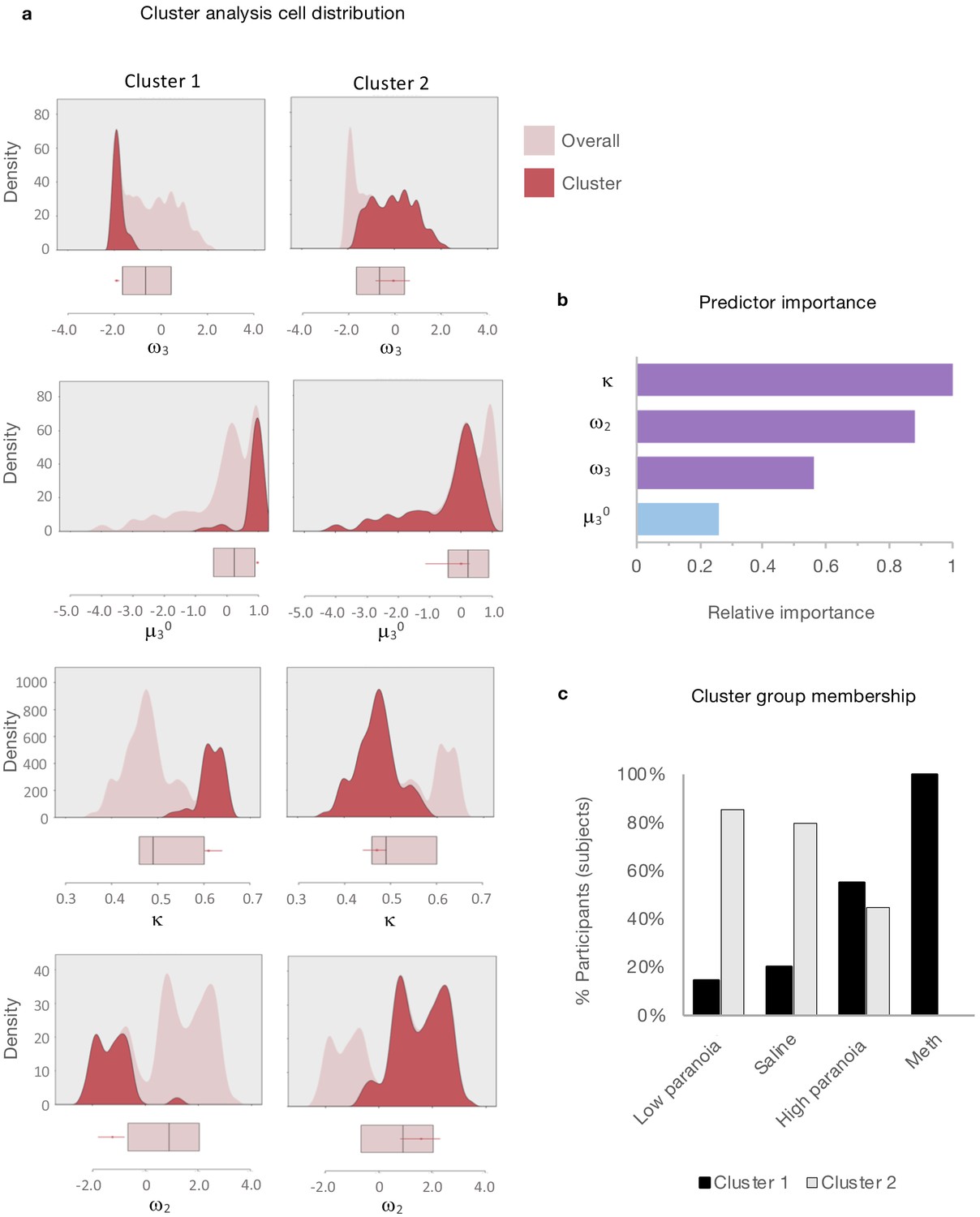
Cluster analysis of HGF parameters.
Two-step cluster analysis of model parameters (ω3, μ30, κ , ω2) across rat and human data sets (rat, post-Rx; in laboratory and online version 3, block 1). Automated clustering yielded an optimal two clusters with good cohesion and separation (average silhouette coefficient = 0.7; cluster size ratio = 2.46). (a) Density plots for μ30, κ, ω2, and ω3 (light pink) depict cluster-specific distributions for each parameter (red). Unlike frequency histograms (that depict the number of data points in bins), density plots employ smoothing to prioritize distribution shape and are not restricted by bin size. Beneath each density plot, box-plots of overall median, 25th quartile, and 75th quartile for each parameter are aligned (pink), with cluster medians and quartiles superimposed (red). Relative to the overall distribution, Cluster 1 (n = 35) medians are elevated for μ30 and κ, decreased for ω2 and ω3. Cluster 2 (n = 86) falls within each overall distribution. (b) Predictor importance of included parameters. Consistent with the color scheme in Figure 2a, Uncertainty weighting parameters (κ, ω2, ω3 ) are depicted in purple and μ30 the prior is in blue. (c) Distribution of cluster identities within groups. Black bars signify the proportion of group members assigned to Cluster one and gray bars represent the proportion of group members assigned to Cluster 2. Cluster one membership is significantly associated with paranoia and methamphetamine groups (χ2(1, n = 121)=29.447, p=5.75E-8). Columns display means [standard error] or percentage of participants within the described category, test-statistics, and p-values. †Independent samples t-test: t-value (df). Two-tailed P-values reported. ‡Chi square coefficient (df). §Fisher’s exact test, exact significance (2-sided). ¶Equal variances not assumed. #Not significant (Bonferonni correction). ††Data presented in Figure 8; repeated measures ANOVA, paranoia group trend or effect: F(df), P; estimated marginal means and standard error. ‡‡Data presented in Figure 2; repeated measures ANOVA, F(df), P. In laboratory: paranoia x block interactions for ω3, μ30; paranoia group effects for κ, ω2. Version 3: paranoia group effects reported. See Table 3 for complete ANOVA. results. Version columns display means [standard error] or percentage of participants within the described category. ††Univariate analysis, F(df). ‡Exact test, chi-square coefficient (df). § Exact significance (2-sided). ||Monte Carlo significance (2-sided). ‡‡Data presented in Figure 3; repeated measures ANOVA, F(df), P. Mean values collapsed across blocks.
Tables
Table 1
In Lab vs. Online Version 3.
| In Lab | Online Version 3 | |||||||
|---|---|---|---|---|---|---|---|---|
| Low Paranoia (n=21) | High Paranoia (n=11) | Statistic | p-value | Low Paranoia (n=56) | High Paranoia (n=16) | Statistic | p-value | |
| Demographics | ||||||||
| Age (years) | 36.0 [3.2] | 38.9 [3.9] | -0.531 (27)† | 0.6 | 38.6 [1.6] | 32.9 [1.7] | 2.441 (41.8)† | 0.019¶ |
| Gender | 0.006 (1)‡ | 1§ | .780 (1)‡ | 0.410 | ||||
| % Female | 71.4% | 72.7% | n/a | n/a | 50.0% | 62.5% | n/a | n/a |
| % Male | 28.6% | 27.3% | n/a | n/a | 50.0% | 37.5% | n/a | n/a |
| % Other or not specified | 0% | 0% | n/a | n/a | 0% | 0% | n/a | n/a |
| Education | 4.972 (6)‡ | 0.638§ | 5.351 (6)‡ | 0.549§ | ||||
| % High school degree or equivalent | 19.0% | 45.5% | n/a | n/a | 16.1% | 6.3% | n/a | n/a |
| % Some college or university, no degree | 14.3% | 0% | n/a | n/a | 17.9% | 25.0% | n/a | n/a |
| % Associate degree | 9.5% | 9.1% | n/a | n/a | 12.5% | 12.5% | n/a | n/a |
| % Bachelor's degree | 23.8% | 27.3% | n/a | n/a | 35.7% | 56.3% | n/a | n/a |
| % Master's degree | 9.5% | 0% | n/a | n/a | 14.3% | 0% | n/a | n/a |
| % Doctorate or professional degree | 4.8% | 0% | n/a | n/a | 1.8% | 0% | n/a | n/a |
| % Completed some postgraduate | 0% | 0% | n/a | n/a | 1.8% | 0% | n/a | n/a |
| % Other / not specified | 19.0% | 18.2% | n/a | n/a | 0% | 0% | n/a | n/a |
| Ethnicity | .134 (1)‡ | 1§ | .117 (1)‡ | 1§ | ||||
| % Hispanic, Latino, or Spanish origin | 23.8% | 18.2% | n/a | n/a | 8.9% | 6.3% | n/a | n/a |
| % Not of Hispanic, Latino, or Spanish origin | 76.2% | 81.8% | n/a | n/a | 91.1% | 93.8% | n/a | n/a |
| Race | 6.250 (4)‡ | 0.186§ | 5.368 (4)‡ | 0.229§ | ||||
| % White | 61.9% | 36.4% | n/a | n/a | 85.7% | 75.0% | n/a | n/a |
| % Black or African American | 19.0% | 36.4% | n/a | n/a | 0% | 12.5% | n/a | n/a |
| % Asian | 14.3% | 9.1% | n/a | n/a | 3.6% | 6.3% | n/a | n/a |
| % American Indian or Alaska Native | 4.8% | 0% | n/a | n/a | 1.8% | 6.3% | n/a | n/a |
| % Multiracial | 0% | 0% | n/a | n/a | 3.6% | 0% | n/a | n/a |
| % Other / not specified | 0% | 18.2% | n/a | n/a | 5.4% | 0% | n/a | n/a |
| Mental Health | ||||||||
| Psychiatric diagnosis | 12.329 (2)‡ | 0.002§ | 7.850 (3)‡ | 0.039§ | ||||
| % No psychiatric diagnosis | 71.4% | 9.1% | adj. residuals | 0.004 | 71.4% | 50.0% | adj. residuals | 0.465 |
| % Schizophrenia spectrum | 19.0% | 36.4% | adj. residuals | 0.546 | 0% | 6.3% | adj. residuals | 0.307 |
| % Mood disorder | 9.5% | 54.5% | adj. residuals | 0.020# | 21.4% | 43.8% | adj. residuals | 0.356 |
| % Not specified | 0% | 0% | adj. residuals | n/a | 7.1% | 0% | adj. residuals | 0.751 |
| % Medicated | 23.8% | 81.8% | 9.871 (1)‡ | 0.003§ | 7.1% | 31.3% | 8.730 (2)‡ | 0.023§ |
| Beck's Anxiety Inventory | 0.27 [0.08] | 0.85 [0.17] | -3.453 (30)† | 0.002 | 0.24 [0.04] | 0.90 [0.20] | -3.303 (16.179)† | 0.004¶ |
| Beck's Depression Inventory | 0.23 [0.05] | 0.66 [0.15] | -2.67 (11.854)† | 0.021¶ | 0.25 [0.04] | 1.03 [0.19] | -3.951 (16.659)† | 0.001¶ |
| SCID Paranoia Personality Score | 0.09 [0.02] | 0.63 [0.04] | -13.476 (30)† | 2.92E-14 | 0.1 [0.02] | 0.72 [0.04] | -16.551 (70)† | 6.712E-26 |
| Reversal Learning Performance | ||||||||
| Total points earned | 7061.9 [286.9] | 6290.9 [372.2] | 1.608 (30)† | 0.118 | 7533.0 [143.8] | 6503.1 [340.6] | 3.177 (70)† | 0.002 |
| Total reversals achieved | 4.8 [0.7] | 2.5 [0.8] | 2.145 (30)† | 0.04 | 6.3 [0.3] | 4.9 [0.8] | 1.758 (20.14)† | 0.094¶ |
| % Achieving reversals | 90.5% | 72.7% | 1.407 (1)‡ | 0.327§ | 100% | 87.5% | 7.200 (1)‡ | 0.047§ |
| Trials to first reversal | 29.2 [4.5] | 27.9 [11] | 0.136 (25)† | 0.893 | 20.0 [1.7] | 13.7 [1.8] | 1.774 (68)† | 0.081 |
| % Recovering post-reversal | 81.0% | 54.5% | 2.490 (1)‡ | 0.213§ | 91.1% | 69.0% | 3.482 (1)‡ | 0.097§ |
| Trials to switch | 1.68 [0.22] | 1.43 [0.20] | 0.671 (24)† | 0.509 | 2.1 [0.2] | 2.6 [0.6] | -1.088 (64)† | 0.280 |
| Trials to recovery | 3.75 [0.51] | 4 [0.93] | -0.285 (21)† | 0.779 | 2.9 [0.3] | 4.9 [0.8] | -2.694 (60)† | 0.009 |
| Win-switch rate, block 1 (90-50-10) | 0.08 [0.03] | 0.24 [0.09] | -1.742 (12.379)† | 0.106¶ | 0.04 [0.01] | 0.13 [0.05] | -1.906 (15.762)† | 0.075¶ |
| Win-switch rate, block 2 (80-40-20) | 0.07 [0.04] | 0.21 [0.1] | -1.601 (30)† | 0.12 | 0.02 [0.01] | 0.12 [0.05] | -2.02 (15.915)† | 0.061¶ |
| Lose-stay rate, block 1 (90-50-10) | 0.19 [0.03] | 0.13 [0.06] | 0.919 (30)† | 0.365 | 0.30 [0.03] | 0.39 [0.06] | -1.425 (70)† | 0.158 |
| Lose-stay rate, block 2 (80-40-20) | 0.26 [0.05] | 0.12 [0.05] | 1.817 (30)† | 0.079 | 0.33 [0.03] | 0.37 [0.06] | -0.554 (70)† | 0.581 |
| Null trials | 8.5 [2.8] | 10.4 [3.7] | -0.391 (30)† | 0.699 | n/a | n/a | n/a | n/a |
-
† Independent samples t-test: t-value (df). Two-tailed p-values reported ‡ Exact test, chi-square coefficient (df)§ Exact significance (2-sided)¶ Equal variances not assumed # Not significant (bonferonni correction).
Table 2
Online experiment.
| Version 1 | Version 2 | Version 3 | Version 4 | Version Effect | Paranoia Effect | Interaction | ||||||||
|---|---|---|---|---|---|---|---|---|---|---|---|---|---|---|
| Low Paranoia (n=45) | High Paranoia (n=20) | Low Paranoia (n=69) | High Paranoia (n=18) | Low Paranoia (n=56) | High Paranoia (n=16) | Low Paranoia (n=64) | High Paranoia (n=19) | Statistic | p-value | Statistic | p-value | Statistic | p-value | |
| Demographics | ||||||||||||||
| Age (years) | 36.5 [1.5] | 35.4 [2.4] | 36.2 [1.4] | 39.5 [2.8] | 38.6 [1.6] | 32.9 [1.7] | 37.6 [1.3] | 30.7 [1.6] | 1.12 (3)†† | 0.342 | 3.202 (1)†† | 0.075 | 2.619 (3)†† | 0.051 |
| Gender | 7.29 (6)‡ | 0.238§ | 1.373 (2)‡ | 0.503§ | n/a | n/a | ||||||||
| % Female | 44.4% | 45.0% | 47.8% | 50.0% | 50.0% | 62.5% | 57.8% | 73.7% | n/a | n/a | n/a | n/a | n/a | n/a |
| % Male | 55.6% | 55.0% | 50.7% | 50.0% | 50.0% | 37.5% | 42.2% | 26.3% | n/a | n/a | n/a | n/a | n/a | n/a |
| % Other or not specified | 0% | 0% | 1.4% | 0% | 0% | 0% | 0% | 0% | n/a | n/a | n/a | n/a | n/a | n/a |
| Education | 15.9 (21)‡ | 0.812|| | 7.326 (7)‡ | 0.4§ | n/a | n/a | ||||||||
| % High school degree or equivalent | 17.8% | 20.0% | 13.0% | 16.7% | 16.1% | 6.3% | 25.0% | 10.5% | n/a | n/a | n/a | n/a | n/a | n/a |
| % Some college or university, no degree | 22.2% | 30.0% | 24.6% | 22.2% | 17.9% | 25.0% | 25.0% | 26.3% | n/a | n/a | n/a | n/a | n/a | n/a |
| % Associate degree | 13.3% | 15.0% | 17.4% | 22.2% | 12.5% | 12.5% | 9.4% | 21.1% | n/a | n/a | n/a | n/a | n/a | n/a |
| % Bachelor's degree | 33.3% | 35.0% | 40.6% | 22.2% | 35.7% | 56.3% | 28.1% | 31.6% | n/a | n/a | n/a | n/a | n/a | n/a |
| % Master's degree | 8.9% | 0% | 2.9% | 0% | 14.3% | 0% | 7.8% | 10.5% | n/a | n/a | n/a | n/a | n/a | n/a |
| % Doctorate or professional degree | 4.4% | 0% | 0% | 5.6% | 1.8% | 0% | 1.6% | 0% | n/a | n/a | n/a | n/a | n/a | n/a |
| % Completed some postgraduate | 0% | 0% | 1.4% | 5.6% | 1.8% | 0% | 3.1% | 0% | n/a | n/a | n/a | n/a | n/a | n/a |
| % Other / not specified | 0% | 0% | 0% | 5.6% | 0% | 0% | 0% | 0% | n/a | n/a | n/a | n/a | n/a | n/a |
| Income | 14.961 (18)‡ | .671|| | 1.177 (6)‡ | 0.981§ | n/a | n/a | ||||||||
| Less than $20,000 | 24.4% | 25.0% | 24.6% | 33.3% | 17.9% | 37.5% | 23.4% | 15.8% | n/a | n/a | n/a | n/a | n/a | n/a |
| $20,000 to $34,999 | 40.0% | 25.0% | 20.3% | 22.2% | 33.9% | 31.3% | 28.1% | 31.6% | n/a | n/a | n/a | n/a | n/a | n/a |
| $35,000 to $49,999 | 15.6% | 15.0% | 18.8% | 16.7% | 12.5% | 6.3% | 18.8% | 15.8% | n/a | n/a | n/a | n/a | n/a | n/a |
| $50,000 to $74,999 | 13.3% | 35.0% | 20.3% | 5.6% | 21.4% | 12.5% | 18.8% | 21.1% | n/a | n/a | n/a | n/a | n/a | n/a |
| $75,000 to $99,999 | 4.4% | 0% | 7.2% | 11.1% | 8.9% | 6.3% | 7.8% | 15.8% | n/a | n/a | n/a | n/a | n/a | n/a |
| Over $100,000 | 0% | 0% | 5.8% | 5.6% | 3.6% | 6.3% | 1.6% | 0% | n/a | n/a | n/a | n/a | n/a | n/a |
| Not specified | 2.2% | 0% | 2.9% | 5.6% | 1.8% | 0% | 1.6% | 0% | n/a | n/a | n/a | n/a | n/a | n/a |
| Cognitive Reflection | 11.922 (9)‡ | 0.223|| | 7.002 (3)‡ | 0.071§ | n/a | n/a | ||||||||
| % Answering 0/3 correctly | 11.1% | 25.0% | 10.1% | 11.1% | 17.9% | 25.0% | 15.6% | 26.3% | n/a | n/a | n/a | n/a | n/a | n/a |
| % Answering 1/3 correctly | 4.4% | 5.0% | 15.9% | 11.1% | 8.9% | 25.0% | 14.1% | 15.8% | n/a | n/a | n/a | n/a | n/a | n/a |
| % Answering 2/3 correctly | 13.3% | 25.0% | 15.9% | 16.7% | 19.6% | 25.0% | 21.9% | 31.6% | n/a | n/a | n/a | n/a | n/a | n/a |
| % Answering 3/3 correctly | 71.1% | 45.0% | 58.0% | 61.1% | 53.6% | 25.0% | 48.4% | 26.3% | n/a | n/a | n/a | n/a | n/a | n/a |
| Ethnicity | 5.162 (3)‡ | 0.157§ | 3.715 (1)‡ | 0.069§ | n/a | n/a | ||||||||
| % Hispanic, Latino, or Spanish origin | 4.4% | 15.0% | 1.4% | 0% | 8.9% | 6.3% | 1.6% | 15.8% | n/a | n/a | n/a | n/a | n/a | n/a |
| % Not of Hispanic, Latino, or Spanish origin | 95.6% | 85.0% | 98.6% | 100.0% | 91.1% | 93.8% | 98.4% | 84.2% | n/a | n/a | n/a | n/a | n/a | n/a |
| Race | 19.559 (15)‡ | .173|| | 9.626 (5)‡ | 0.084§ | n/a | n/a | ||||||||
| % White | 82.2% | 75.0% | 84.1% | 88.9% | 85.7% | 75.0% | 85.9% | 73.7% | n/a | n/a | n/a | n/a | n/a | n/a |
| % Black or African American | 6.7% | 15.0% | 5.8% | 11.1% | 0% | 12.5% | 4.7% | 10.5% | n/a | n/a | n/a | n/a | n/a | n/a |
| % Asian | 8.9% | 10.0% | 7.2% | 0% | 3.6% | 6.3% | 7.8% | 0% | n/a | n/a | n/a | n/a | n/a | n/a |
| % American Indian or Alaska Native | 0% | 0% | 0% | 0% | 1.8% | 6.3% | 0% | 0% | n/a | n/a | n/a | n/a | n/a | n/a |
| % Multiracial | 2.2% | 0% | 1.4% | 0% | 3.6% | 0% | 1.6% | 15.8% | n/a | n/a | n/a | n/a | n/a | n/a |
| % Other / not specified | 0% | 0% | 1.4% | 0% | 5.4% | 0% | 0% | 0% | n/a | n/a | n/a | n/a | n/a | n/a |
| Mental Health | ||||||||||||||
| Psychiatric diagnosis | 10.783 (9)‡ | 0.292|| | 2.960 (3)‡ | 0.361§ | n/a | n/a | ||||||||
| % No psychiatric diagnosis | 73.3% | 80.0% | 60.9% | 55.6% | 71.4% | 50.0% | 65.6% | 42.1% | n/a | n/a | n/a | n/a | n/a | n/a |
| % Schizophrenia spectrum | 2.2% | 0% | 0% | 0% | 0% | 6.3% | 0% | 0% | n/a | n/a | n/a | n/a | n/a | n/a |
| % Mood disorder | 13.3% | 15.0% | 27.5% | 22.2% | 21.4% | 43.8% | 26.6% | 31.6% | n/a | n/a | n/a | n/a | n/a | n/a |
| % Not specified | 11.1% | 5.0% | 11.6% | 22.2% | 7.1% | 0% | 7.8% | 26.3% | n/a | n/a | n/a | n/a | n/a | n/a |
| % Medicated | 8.9% | 10.0% | 13.0% | 22.2% | 7.1% | 31.3% | 14.1% | 10.5% | 3.575 (6)‡ | 0.744§ | 4.164 (2)‡ | 0.121§ | n/a | n/a |
| Beck's Anxiety Inventory | 0.34 [0.06] | 0.52 [0.14] | 0.31 [0.04] | 0.6 [0.13] | 0.24 [0.04] | 0.90 [0.20] | 0.33 [0.06] | 0.79 [0.18] | 1.244 (3)† | 0.2941 | 38.752 (1)†† | 1.63E-09 | 2.577 (3)†† | 0.0539 |
| Beck's Depression Inventory | 0.36 [0.07] | 0.86 [0.15] | 0.32 [0.05] | 0.79 [0.13] | 0.25 [0.04] | 1.03 [0.19] | 0.38 [0.07] | 1.06 [0.20] | 1.023 (3)† | 0.3827 | 74.528 (1)†† | 3.62E-16 | 1.089 (3)†† | 0.3542 |
| SCID Paranoia Personality Score | 0.11 [0.02] | 0.67 [0.04] | 0.11 [0.02] | 0.61 [0.03] | 0.1 [0.02] | 0.72 [0.04] | 0.11 [0.02] | 0.65 [0.03] | 1.297 (3)† | 0.2756 | 879.379 (1)†† | 4.81E-91 | 2.018 (3)†† | 0.1114 |
| Reversal Learning Performance | ||||||||||||||
| Total points earned | 8656.7 [182.9] | 8372.5 [405.2] | 6045.7 [135.7] | 6266.7 [288.0] | 7533.0 [143.8] | 6503.1 [340.6] | 7171.1 [175.6] | 6510.5 [403.6] | 32.288 (3)† | 4.16E-18 | 6.175 (1)†† | 0.0135 | 2.258 (3)†† | 0.0818 |
| Total reversals achieved | 7.2 [0.3] | 6.5 [0.5] | 5.5 [0.3] | 5.7 [0.5] | 6.3 [0.3] | 4.9 [0.8] | 5.9 [0.3] | 4.8 [0.6] | 4.329 (3)† | 0.005 | 5.762 (1)†† | 0.017 | 1.101 (3)†† | 0.349 |
| % Achieving reversals | 100% | 100% | 98.6% | 94.4% | 100% | 87.5% | 96.9% | 94.7% | 2.26 (3)‡ | 0.598§ | 4.4 (1)‡ | 0.058§ | n/a | n/a |
| Win-switch rate, block 1 (90-50-10) | 0.09 [0.03] | 0.09 [0.04] | 0.07 [0.01] | 0.11 [0.05] | 0.04 [0.01] | 0.13 [0.05] | 0.1 [0.03] | 0.21 [0.06] | 2.284 (3)† | 0.079 | 7.117 (1)†† | 0.008 | 1.15 (3)†† | 0.329 |
| Win-switch rate, block 2 (80-40-20) | 0.05 [0.02] | 0.08 [0.03] | 0.04 [0.01] | 0.05 [0.04] | 0.02 [0.01] | 0.12 [0.05] | 0.06 [0.02] | 0.15 [0.05] | 2.067 (3)† | 0.105 | 9.918 (1)†† | 0.002 | 1.174 (3)†† | 0.32 |
| Lose-stay rate, block 1 (90-50-10) | 0.27 [0.03] | 0.34 [0.05] | 0.37 [0.03] | 0.34 [0.04] | 0.3 [0.03] | 0.39 [0.06] | 0.32 [0.03] | 0.34 [0.04] | 0.561 (3)† | 0.641 | 1.834 (1)†† | 0.177 | 0.754 (3)†† | 0.521 |
| Lose-stay rate, block 2 (80-40-20) | 0.28 [0.03] | 0.23 [0.05] | 0.4 [0.03] | 0.32 [0.05] | 0.33 [0.03] | 0.37 [0.06] | 0.29 [0.03] | 0.33 [0.06] | 2.47 (3)† | 0.062 | 0.177 (1)†† | 0.674 | 0.834 (3)†† | 0.476 |
| Reaction time, block 1 | 433.6 [28.8] | 789.3 [282.7] | 548.1 [77.8] | 365.6 [26.4] | 448 [60.1] | 442.1 [59.5] | 557.2 [108.2] | 530 [130.2] | 0.793 (3)† | 0.499 | 0.161 (1)†† | 0.689 | 1.727 (3)†† | 0.161 |
| Reaction time, block 2 | 370.7 [23.3] | 494.3 [88.6] | 465.3 [61.6] | 331.4 [22.9] | 391.7 [52.3] | 555.9 [121.2] | 385.4 [29.2] | 504.1 [82.7] | 0.394 (3)† | 0.757 | 1.92 (1)†† | 0.167 | 1.949 (3)†† | 0.122 |
-
† Univariate analysis, F(df) with df error = 306 Exact test, ‡chi-square coefficient (df), § Exact significance (2-sided), || Monte Carlo significance (2-sided).
Table 3
ANOVA results for HGF parameters.
| Block effect † | Group effect‡ | Interaction effect | ||||
|---|---|---|---|---|---|---|
| Statistic§ | p-value | Statistic§ | p-value | Statistic§ | p-value | |
| Experiment 1 | ||||||
| ω3 | 11.672 (1) | 0.002 | 1.294 (1) | 0.264 | 6.948 (1) | 0.013 |
| µ30 | 25.904 (1) | 1.809E-5 | 7.063 (1) | 0.012 | 5.344 (1) | 0.028 |
| κ | 7.768 (1) | 0.009 | 7.599 (1) | 0.010 | 0.003 (1) | 0.960 |
| ω2 | 2.182 (1) | 0.150 | 4.186 (1) | 0.050 | 0.058 (1) | 0.811 |
| µ20 | 4.831 (1) | 0.036 | 1.261 (1) | 0.270 | 0.370 (1) | 0.547 |
| BIC | 0.061 (1) | 0.807 | 8.801 (1) | 0.006 | 1.7 (1) | 0.202 |
| Experiment 2, Version 3 | ||||||
| ω3 | 14.932 (1) | 0.0002 | 1.128 (1) | 0.292 | 1.406 (1) | 0.240 |
| µ30 | 64.651 (1) | 1.54E-11 | 6.366 (1) | 0.014 | 0.003 (1) | 0.959 |
| κ | 15.53 (1) | 0.0002 | 13.521 (1) | 0.0005 | 0.011 (1) | 0.916 |
| ω2 | 0.027 (1) | 0.869 | 8.70 (1) | 0.004 | 0.090 (1) | 0.765 |
| µ20 | 11.432 (1) | 0.001 | 0.030 (1) | 0.864 | 0.203 (1) | 0.653 |
| BIC | 1.110E-5 (1) | 0.997 | 16.336 (1) | 0.0001 | 1.678 (1) | 0.199 |
| Experiment 3: Rats | ||||||
| ω3 | 30.086 (1) | 6.2785E-5 | 4.579 (1) | 0.049 | 9.058 (1) | 0.009 |
| µ30 | 31.416 (1) | 5.0188E-5 | 8.454 (1) | 0.011 | 5.159 (1) | 0.038 |
| κ | 9.132 (1) | 0.009 | 13.356 (1) | 0.002 | 2.644 (1) | 0.125 |
| ω2 | 32.192 (1) | 4.4173E-5 | 22.344 (1) | 0.0003 | 18.454 (1) | 0.001 |
| µ20 | 5.226 (1) | 0.037 | 0.368 (1) | 0.553 | 2.087 (1) | 0.169 |
| BIC | 5.052 (1) | 0.040 | 1.890 (1) | 0.189 | 0.331 (1) | 0.573 |
-
Block refers to first versus second half in human studies, Pre-Rx vs Post-Rx in rat studies.‡ Group refers to low versus high paranoia in humans, saline versus methamphetamine in rats §F-statistic (degrees of freedom); df error = 30 in Experiment 1, 70 in Experiment 2, Version 3, and 50 in Experiment 3: Rats; split-plot ANOVA (i.e., repeated measures with between-subjects factor).
Table 4
Corrections for multiple comparisons.
| Group effect † | Interaction effect‡ | |||||||
|---|---|---|---|---|---|---|---|---|
| Survives bonferroni?§ | Survives FDR? | Critical value | Benjamini-Hochberg p-value | Survives bonferroni?§ | Survives FDR? | Critical value | Benjamini-Hochberg p-value | |
| Experiment 1 | ||||||||
| ω3 | N/A | N/A | 0.05 | 0.264 | No | No | 0.0125 | 0.052 |
| µ30 | Yes | Yes | 0.025 | 0.024 | No | No | 0.025 | 0.056 |
| κ | Yes | Yes | 0.0125 | 0.04 | N/A | N/A | 0.05 | 0.96 |
| ω2 | No | No | 0.0375 | 0.0667 | N/A | N/A | 0.0375 | 1.081 |
| Experiment 2, Version 3 | ||||||||
| ω3 | N/A | N/A | 0.05 | 0.292 | N/A | N/A | 0.0125 | 0.96 |
| µ30 | No | Yes | 3.75E-02 | 0.0187 | N/A | N/A | 0.05 | 0.959 |
| κ | Yes | Yes | 0.0125 | 0.002 | N/A | N/A | 0.0375 | 1.221 |
| ω2 | Yes | Yes | 0.025 | 0.008 | N/A | N/A | 0.025 | 1.53 |
| Experiment 3: Rats | ||||||||
| ω3 | No | Yes | 5.00E-02 | 0.049 | Yes | Yes | 0.025 | 0.018 |
| µ30 | Yes | Yes | 3.75E-02 | 0.0147 | No | No | 0.0375 | 0.0507 |
| κ | Yes | Yes | 0.025 | 0.004 | N/A | N/A | 0.05 | 0.125 |
| ω2 | Yes | Yes | 0.0125 | 0.0012 | Yes | Yes | 0.0125 | 0.004 |
-
N/A denotes to p-values that were not significant before corrections. † Low versus high paranoia in humans, saline versus methamphetamine in rats. ‡ Group by time (i.e., first versus second half in human studies, Pre-Rx vs Post-Rx in rat studies). § p-value < 0.0125.
Table 5
Experiment 2 effects across block, paranoia group, and task version.
| Block | Group | Version | Block*group* Version | Group*version | Block*group | Block*version | ||||||||
|---|---|---|---|---|---|---|---|---|---|---|---|---|---|---|
| F (df)† | P | F (df)† | P | F (df)† | P | F (df)† | P | F (df)† | P | F (df)† | P | F (df)† | P | |
| ω3 | 3.722 (1) | 0.055 | 0.499 (1) | 0.481 | 2.061 (3) | 0.105 | 0.415 (3) | 0.742 | 1.005 (3) | 0.391 | 0.145 (1) | 0.704 | 7.0155 (3) | 1.42E-4 |
| µ30 | 288.1 (1) | 1.01E-45 | 2.604 (1) | 0.108 | 2.321 (3) | 0.075 | 0.261 (3) | 0.853 | 2.329 (3) | 0.075 | 0.281 (1) | 0.597 | 0.061 (3) | 0.98 |
| κ | 120.9 (1) | 7.65E-24 | 3.602 (1) | 0.059 | 5.06 (3) | 0.002 | 0.08 (3) | 0.971 | 4.178 (3) | 0.006 | 1.028 (1) | 0.312 | 2.559 (3) | 0.055 |
| ω2 | 35.3 (1) | 7.92E-9 | 4.435 (1) | 0.036 | 4.155 (3) | 0.007 | 0.166 (3) | 0.919 | 2.809 (3) | 0.04 | 2.387 (1) | 0.123 | 8.697 (3) | 1.5E-5 |
| µ20 | 71.3 (1) | 1.33E-15 | 0.242 (1) | 0.623 | 0.616 (3) | 0.605 | 1.081 (3) | 0.358 | 0.412 (3) | 0.744 | 0.057 (1) | 0.812 | 1.505 (3) | 0.213 |
| BIC | 56.6 (1) | 6.23E-13 | 8.073 (1) | 0.005 | 5.385 (3) | 0.001 | 0.262 (3) | 0.853 | 4.927 (3) | 0.002 | 0.451 (1) | 0.502 | 11.905 (3) | 2.19E-07 |
-
† F-statistic (degrees of freedom); df error = 299; split-plot ANOVA (i.e., repeated measures with two between-subjects factors).
N/A denotes to p-values that were not significant before corrections. † Low versus high paranoia in humans, saline versus methamphetamine in rats. ‡ Group by time (i.e., first versus second half in human studies, Pre-Rx vs Post-Rx in rat studies). § p-value < 0.0125.
Table 6
Experiment 2 ANCOVAs.
| ω3 | µ30 | κ | ω2 | ||||||
|---|---|---|---|---|---|---|---|---|---|
| Effect | Df | F | p-value | F | p-value | F | p-value | F | p-value |
| Demographics (age, gender, ethnicity, and race) | |||||||||
| Block | 1, 294 | 0.328 | 0.568 | 10.835 | 0.001 | 3.425 | 0.066 | 2.711 | 0.101 |
| Block * Age | 1, 294 | 0.659 | 0.418 | 2.035 | 0.155 | 2.195 | 0.14 | 0.212 | 0.646 |
| Block * Gender | 1, 294 | 0.363 | 0.547 | 0.105 | 0.746 | 4.042 | 0.046 | 0.096 | 0.757 |
| Block * Ethnicity | 1, 294 | 0.016 | 0.901 | 0.042 | 0.837 | 0.268 | 0.605 | 0.024 | 0.876 |
| Block * Race | 1, 294 | 3.244 | 0.073 | 0.279 | 0.598 | 0.082 | 0.775 | 1.386 | 0.24 |
| Block * Paranoia Group | 1, 294 | 0.001 | 0.969 | 0.162 | 0.687 | 0.738 | 0.391 | 1.189 | 0.277 |
| Block * Version | 3, 294 | 7.61 | 7.25E-05 | 0.561 | 0.641 | 2.568 | 0.055 | 8.613 | 1.97E-05 |
| Block * Paranoia Group * Version | 3, 294 | 0.451 | 0.717 | 0.135 | 0.939 | 0.119 | 0.949 | 0.1 | 0.96 |
| Age | 1, 294 | 3.054 | 0.082 | 2.974 | 0.086 | 2.101 | 0.149 | 2.339 | 0.128 |
| Gender | 1, 294 | 0.438 | 0.509 | 0.02 | 0.886 | 0.005 | 0.941 | 0.014 | 0.905 |
| Ethnicity | 1, 294 | 0.029 | 0.865 | 0.059 | 0.808 | 0.087 | 0.768 | 0.221 | 0.639 |
| Race | 1, 294 | 0.072 | 0.789 | 2.218 | 0.138 | 0.373 | 0.542 | 0.333 | 0.564 |
| Paranoia Group | 1, 294 | 4.71E-04 | 0.983 | 0.741 | 0.39 | 1.795 | 0.182 | 3.302 | 0.071 |
| Version | 3, 294 | 1.845 | 0.14 | 1.914 | 0.128 | 4.975 | 0.002 | 3.786 | 0.011 |
| Paranoia Group * Version | 3, 294 | 0.935 | 0.424 | 1.911 | 0.129 | 3.599 | 0.014 | 1.919 | 0.127 |
| Mental health factors (medication usage, diagnostic category, BAI score, and BDI score) | |||||||||
| Block | 1, 257 | 3.333 | 0.069 | 95.753 | 3.12E-19 | 25.498 | 8.78E-07 | 8.341 | 0.004 |
| Block * BAI | 1, 257 | 0.26 | 0.611 | 1.532 | 0.217 | 2.852 | 0.093 | 0.394 | 0.531 |
| Block * BDI | 1, 257 | 0.009 | 0.926 | 0.208 | 0.649 | 6.55 | 0.011 | 0.597 | 0.441 |
| Block * Medication Usage | 1, 257 | 0.027 | 0.87 | 1.288 | 0.258 | 0.691 | 0.407 | 0.871 | 0.352 |
| Block * Diagnostic Category | 1, 257 | 1.366 | 0.244 | 1.785 | 0.183 | 0.063 | 0.803 | 0.208 | 0.649 |
| Block * Paranoia Group | 1, 257 | 0.068 | 0.795 | 0.298 | 0.586 | 0.298 | 0.586 | 0.007 | 0.935 |
| Block * Version | 3, 257 | 5.872 | 0.001 | 0.531 | 0.662 | 0.906 | 0.439 | 6.16 | 0.0005 |
| Block * Paranoia Group * Version | 3, 257 | 1.024 | 0.383 | 0.869 | 0.458 | 0.266 | 0.85 | 0.095 | 0.963 |
| BAI | 1, 257 | 1.108 | 0.294 | 0.012 | 0.913 | 0.954 | 0.33 | 0.921 | 0.338 |
| BDI | 1, 257 | 0.037 | 0.848 | 0.574 | 0.449 | 1.343 | 0.248 | 2.372 | 0.125 |
| Medication Usage | 1, 257 | 0.327 | 0.568 | 0.058 | 0.81 | 0.002 | 0.966 | 0.467 | 0.495 |
| Diagnostic Category | 1, 257 | 4.252 | 0.04 | 0.004 | 0.949 | 1.443 | 0.231 | 1.743 | 0.188 |
| Paranoia Group | 1, 257 | 0.057 | 0.811 | 0.233 | 0.63 | 1.032 | 0.311 | 1.695 | 0.194 |
| Version | 3, 257 | 3.183 | 0.025 | 2.73 | 0.045 | 5.274 | 0.002 | 4.468 | 0.004 |
| Paranoia Group * Version | 3, 257 | 0.311 | 0.818 | 2.307 | 0.077 | 4.556 | 0.004 | 3.397 | 0.019 |
| Global cognitive ability (educational attainment, income, and cognitive reflection) | |||||||||
| Block | 1, 290 | 1.19E-04 | 0.991 | 51.264 | 7.60E-12 | 28.675 | 1.83E-07 | 18.388 | 2.51E-05 |
| Block * Education | 1, 290 | 0.603 | 0.438 | 0.001 | 0.975 | 0.033 | 0.856 | 0.258 | 0.612 |
| Block * Income | 1, 290 | 1.211 | 0.272 | 2.874 | 0.091 | 3.483 | 0.063 | 2.421 | 0.121 |
| Block * Cognitive Reflection | 1, 290 | 1.83 | 0.177 | 0.709 | 0.401 | 1.221 | 0.27 | 4.667 | 0.032 |
| Block * Paranoia Group | 1, 290 | 0.005 | 0.946 | 0.359 | 0.55 | 0.263 | 0.608 | 0.885 | 0.348 |
| Block * Version | 3, 290 | 8.861 | 1.27E-05 | 0.182 | 0.909 | 2.325 | 0.075 | 8.815 | 1.35E-05 |
| Block * Paranoia Group * Version | 3, 290 | 0.826 | 0.48 | 0.478 | 0.698 | 0.15 | 0.929 | 0.3 | 0.825 |
| Education | 1, 290 | 0.111 | 0.739 | 0.578 | 0.448 | 1.395 | 0.239 | 0.608 | 0.436 |
| Income | 1, 290 | 2.763 | 0.098 | 1.382 | 0.241 | 0.055 | 0.814 | 1.035 | 0.31 |
| Cognitive Reflection | 1, 290 | 0.164 | 0.686 | 12.807 | 0.0004 | 0.224 | 0.636 | 0.807 | 0.37 |
| Paranoia Group | 1, 290 | 0.069 | 0.793 | 0.555 | 0.457 | 2.477 | 0.117 | 4.715 | 0.031 |
| Version | 3, 290 | 2.104 | 0.1 | 2.55 | 0.056 | 5.53 | 0.001 | 3.799 | 0.011 |
| Paranoia Group * Version | 3, 290 | 1.288 | 0.279 | 2.568 | 0.055 | 4.469 | 0.004 | 2.793 | 0.041 |
Table 7
Modified Cognitive Reflection Questionnaire Items.
| Item | Prompt |
|---|---|
| 1 | A folder and a paper clip cost $1.10 in total. The folder costs $1.00 more than the paper clip. How much does the paper clip cost? |
| 2 | If it takes 5 clerks 5 min to review five applications, how long would it take 100 clerks to review 100 applications? |
| 3 | In a garden, there is a cluster of weeds. Every day, the cluster doubles in size. If it takes 48 days for the cluster to cover the entire garden, how long would it take for the cluster to cover half of the garden? |
Table 8
Simulations and behavior.
| Win-switch rate | U-value | Lose-stay rate | |||||
|---|---|---|---|---|---|---|---|
| Effect | Df | F | p-value | F | p-value | F | p-value |
| Experiment 1 | |||||||
| Block | 1, 30 | 1.465 | 0.236 | 16.999 | 0.0003 | 1.334 | 0.257 |
| Block*Paranoia Group | 1, 30 | 0.602 | 0.444 | 2.393 | 0.132 | 2.575 | 0.119 |
| Paranoia Group | 1, 30 | 3.579 | 0.068 | 3.312 | 0.079 | 2.283 | 0.141 |
| Experiment 2, Version 3 | |||||||
| Block | 1, 70 | 0.935 | 0.337 | 10.153 | 0.002 | 0.122 | 0.728 |
| Block*Paranoia Group | 1, 70 | 0.001 | 0.982 | 0.003 | 0.958 | 1.93 | 0.169 |
| Paranoia Group | 1, 70 | 12.698 | 0.001 | 19.209 | 4.03E-05 | 1.095 | 0.299 |
| Simulations† | |||||||
| Block | 1, 70 | 0.176 | 0.676 | 3.335 | 0.072 | 5.073 | 0.027 |
| Block*Paranoia Group | 1, 70 | 2.039 | 0.158 | 2.624 | 0.11 | 0.036 | 0.85 |
| Paranoia Group | 1, 70 | 15.394 | 0.0002 | 13.362 | 0.0005 | 0.042 | 0.839 |
-
†Simulated data from experiment 2, Version 3.
Table 9
Alternative models fail to capture paranoia group differences.
| Low Paranoia (n=56)† | High Paranoia (n=16)† | Paranoia Group Effect‡ | Paranoia x Block Effect‡ | ||||||||
|---|---|---|---|---|---|---|---|---|---|---|---|
| Mean | SEM | 95% CI | Mean | SEM | 95% CI | F(df) | P | F(df) | P | ||
| Q-learning with learning rates for positive and negative prediction errors | |||||||||||
| Positive prediction error (α+) | |||||||||||
| 1st half | 0.463 | 0.038 | [0.388, 0.538] | 0.475 | 0.071 | [0.335, 0.616] | 0.243 (1, 70) | 0.623 | 0.118 (1, 70) | 0.732 | |
| 2nd half | 0.476 | 0.039 | [0.398, 0.555] | 0.535 | 0.074 | [0.379, 0.672] | |||||
| Negative prediction error (α-) | |||||||||||
| 1st half | 0.421 | 0.022 | [0.377, 0.464] | 0.365 | 0.041 | [0.284, 0.446] | 1.292 (1, 70) | 0.260 | 0.320 (1, 70) | 0.573 | |
| 2nd half | 0.386 | 0.021 | [0.344, 0.427] | 0.364 | 0.039 | [0.285,0.442] | |||||
| Inverse temperature (β ) | |||||||||||
| 1st half | 271 | 74.0 | [126, 416] | 147 | 133 | [-114, 408] | 1.626 (1, 70) | 0.207 | 0.043 (1, 70) | 0.837 | |
| 2nd half | 316 | 82.3 | [155, 477] | 145 | 132 | [-114, 403] | |||||
| 2-level HGF with softmax decision model | |||||||||||
µ2 | |||||||||||
| 1st half | -0.059 | 0.081 | [-0.218, 0.100] | -0.303 | 0.157 | [-0.611, 0.005] | 3.039 (1, 70) | 0.086 | 0.385 (1, 70) | 0.537 | |
| 2nd half | -0.244 | 0.082 | [-0.405, -0.082] | -0.566 | 0.155 | [-0.869, -0.262] | |||||
| Inverse temperature (β) | |||||||||||
| 1st half | 131 | 30.6 | [71.3, 191] | 35.3 | 6.20 | [23.2, 47.5] | 2.665 (1, 70) | 0.107 | 0.250 (1, 70) | 0.619 | |
| 2nd half | 119 | 30.6 | [58.7, 179] | 52.1 | 12.1 | [28.3, 75.9] | |||||
-
† Online version 3 data ‡ Repeated measures ANOVA.
Table 10
Summary of paranoia/methamphetamine effects on belief-updating.
| In lab | Online | Rats | |
|---|---|---|---|
| ω3 | ↓† | ⇣ | ⬇ |
| µ30 | ⬆ | ⬆‡§ | ⬆ |
| κ | ⬆ | ⬆‡ | ⬆ |
| ω2 | ⬇ | ⬇‡¶ | ⬇ |
| µ02 | - | - | - |
-
⇡ ⇣ Non-significant increase/decrease in high paranoia or meth, relative to low paranoia or saline ↑ ↓ Trend-level increase/decrease in high paranoia or meth, relative to low paranoia or saline ⬆⬇ Significantly higher/lower in high paranoia or meth, relative to low paranoia or saline - - No significant findings or trends † Baseline trend; parameter decreases in second block for low but not high paranoia ‡ Version 3 only § Trend-level significance disappears with inclusion of demographic covariates ¶ Significance reduced to trend with inclusion of demographic covariates.
Table 11
Questionnaire item completion (% responses).
| Questionnaire/subscale | Experiment 1 | Experiment 2 |
|---|---|---|
| Age | 90.6% | 99.7% |
| Gender | 100.0% | 100.0% |
| Ethnicity | 100.0% | 100.0% |
| Race | 100.0% | 100.0% |
| Education | 100.0% | 99.7% |
| Meds | 100.0% | 90.6% |
| Dx | 100.0% | 94.1% |
| Income | N/A | 98.0% |
| SCID-II Paranoia - all items | 96.9% | 94.1% |
| SCID-II Paranoia - one item missing | 3.1% | 5.5% |
| SCID-II Paranoia - three items missing | 0.0% | 0.3% |
| Cognitive reflection - all items | N/A | 97.7% |
| Beck's Anxiety Inventory (BAI) - all items | 90.6% | 96.7% |
| BAI - one item missing | 3.1% | 2.9% |
| BAI - two items missing | 6.3% | 0.3% |
| Beck's Depression Inventory (BDI) - all items | 100.0% | 99.0% |
| BDI - one item missing | 0.0% | 1.0% |
Additional files
Download links
A two-part list of links to download the article, or parts of the article, in various formats.
Downloads (link to download the article as PDF)
Open citations (links to open the citations from this article in various online reference manager services)
Cite this article (links to download the citations from this article in formats compatible with various reference manager tools)
Paranoia as a deficit in non-social belief updating
eLife 9:e56345.
https://doi.org/10.7554/eLife.56345


