Distinct neuronal populations contribute to trace conditioning and extinction learning in the hippocampal CA1
- Department of Biomedical Engineering, Boston University, United States
- Department of Electrical and Computer Engineering, Boston University, United States
Figures
Figure 1 with 1 supplement

Experimental design and quantification of animal behavior.
(A) Imaging and behavioral setup. The imaging setup consisted of a microscope with a sCMOS camera, standard wide-field fluorescence optics, and a 10× long working distance objective to image a head-fixed mouse. For the behavioral paradigm, a speaker was positioned near the mouse and a cannula for directing an air puff was placed in front of one eye. Eye responses were monitored using a USB 3.0 Camera. (B) Experimental timeline. Each animal was injected with AAV-Syn-GCaMP6f and allowed 1–2 weeks for virus expression before surgical window implantation above CA1. The first training session was 4–6 weeks after surgery, and animals were trained and imaged for 5–9 days. (C) Full field of view and selected extracted traces. Maximum-minus-minimum projection image for one motion corrected video to show example field of view of several hundred cells. Inset: several selected cells and their corresponding normalized fluorescence trace recordings. (D) Within trial design. Trials consisted of a 350 ms tone as the conditioned stimulus (CS), followed by a 250 ms trace interval with no sound, followed by a 100 ms puff of air to the eye as the unconditioned stimulus (US). (E) Video eye monitoring and segmentation. (Ei) Raw eye frames aligned to the CS, trace interval, and US windows shown above. (Eii) Eye frames after segmentation. (Eiii) Extracted eye trace and conditioned response (CR) threshold for one trial. (Eiv) Eye trace for all 40 trials of a first training session from one example mouse. Red indicates eye opening, while blue indicates eye closure. (Ev) Extracted eye trace averaged over all trials shown in Eiv.
Figure 1—figure supplement 1
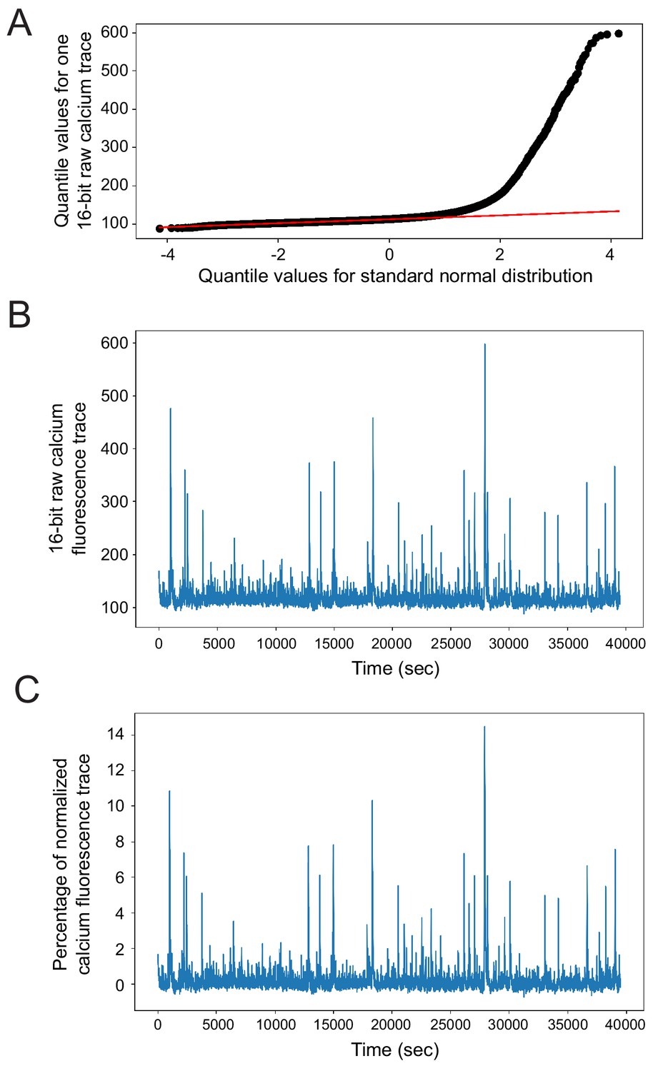
GCaMP6 fluorescence trace normalization and rationale.
(A) Quantile-quantile plot of a representative raw GCaMP6f fluorescence trace vs. a standard normal distribution. Each black dot represents a data point. The raw fluorescence data greatly deviates from fitting a normal distribution at the higher quantiles due to the presence of calcium spiking events. Red line shows a line fit to all the points in the lowest 50th quantile, corresponding GCaMP6 fluorescence baseline noise fluctuations. As this line is straight, it suggests a normal distribution for the baseline noise. The intercept of the red line is thus used to approximate GCaMP6f trace baseline (b0). (B) Raw calcium fluorescence trace over time for the same cell as shown in (A) as recorded by the 16-bit camera. (C) Normalized fluorescence trace for the same cell as in (A) and (B), as normalized by (f - b0) where f is the raw fluorescence as plotted in (B) and b0 is the baseline calculated as in (A).
Figure 2 with 5 supplements
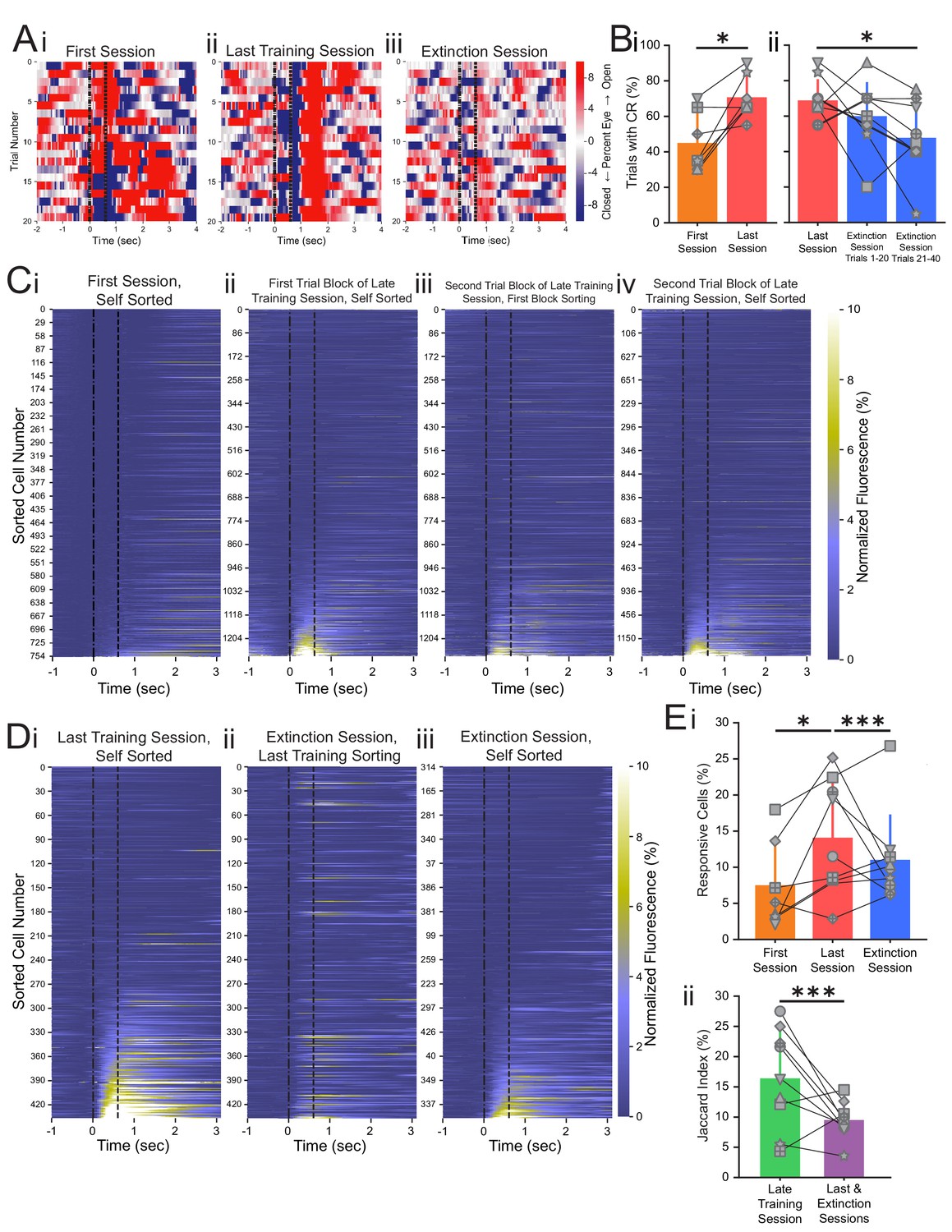
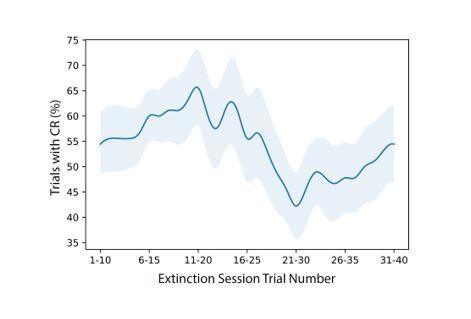
Conditioned responses (CRs) and neuronal calcium responses increase during conditioning and decrease during extinction.
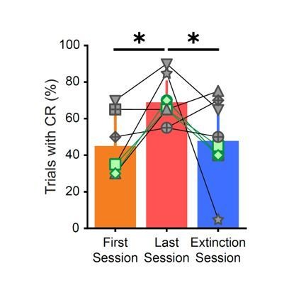
(A) Extracted eye traces across days. Red indicates an increase in eye area, while blue indicates a reduction in eye area. (Ai) Eye trace for 10 tone-only trials and the first 10 trials of the first training session from the same example mouse in Figure 1E. (Aii) Eye trace for the last training session for the same example mouse. (Aiii) Eye trace for the extinction session for the same example mouse. (B) Quantification of CR. (i) Percentage of trials with a CR during the first session (orange) and last training session (red), *p=0.025, n = 7 mice for first vs. last session. (ii) Percentage of trials with a CR during the last session (red), trials 1–20 of the extinction session (blue), and trials 21–40 of the extinction session (blue). p=0.37, n = 9 mice for last session vs. trials 1–20 of extinction session, *p=0.034, n = 9 mice for last session vs. trials 21–40 of extinction session, Wilcoxon rank-sum test. (C) Trial-averaged calcium recordings for the first session and late training session. (Ci) Trial-averaged recordings sorted by average fluorescence between the tone and the puff for the first training session from an example mouse. (Cii) Trial-averaged recordings (plotted as in Ci) for the first trial block of the late training session for the same mouse, sorted by average fluorescence between the tone and the puff for the first trial block of the late training session. (Ciii) Trial-averaged recordings (plotted as in Ci) for the second trial block of the late training session, with cell sorting maintained from the first trial block of the session to identify spatially matched cells. (Civ) The same data as shown in Ciii, but resorted according to the fluorescence between the tone and the puff for the second trial block of the late training session. (D) Trial-averaged calcium recordings for the last training session and extinction session. (Di) Trial-averaged recordings (plotted as in C) for the last training session from the same mouse, sorted by average fluorescence between the tone and the puff for the last training session. (Dii) Trial-averaged recordings (plotted as in Di) of the extinction session, with cell sorting maintained from the last training session to identify spatially matched cells. (Diii) The same data as shown in Dii, but resorted according to the fluorescence between the tone and the puff for the extinction session. (E) Quantification of responsive cell properties. (Ei) Percentage of total cells that are identified as tone-responsive for the first session (orange), last training session (red), and extinction session (blue), **p=0.017, n = 7 mice for first vs. last training session, p=0.92, n = 7 mice for first vs. extinction session, ***p=0.0005, n = 9 mice for last training vs. extinction, Fisher’s exact test. (Eii) Percentage of cells that are present within both responsive cell populations of the first half and last half of the late training session (green) and both responsive cell populations of the last training session and extinction session (purple), ***p=1.88e-6, n = 9 mice, Fisher’s exact test. For all bar plots, error bars are ± s.d.
Figure 2—figure supplement 1
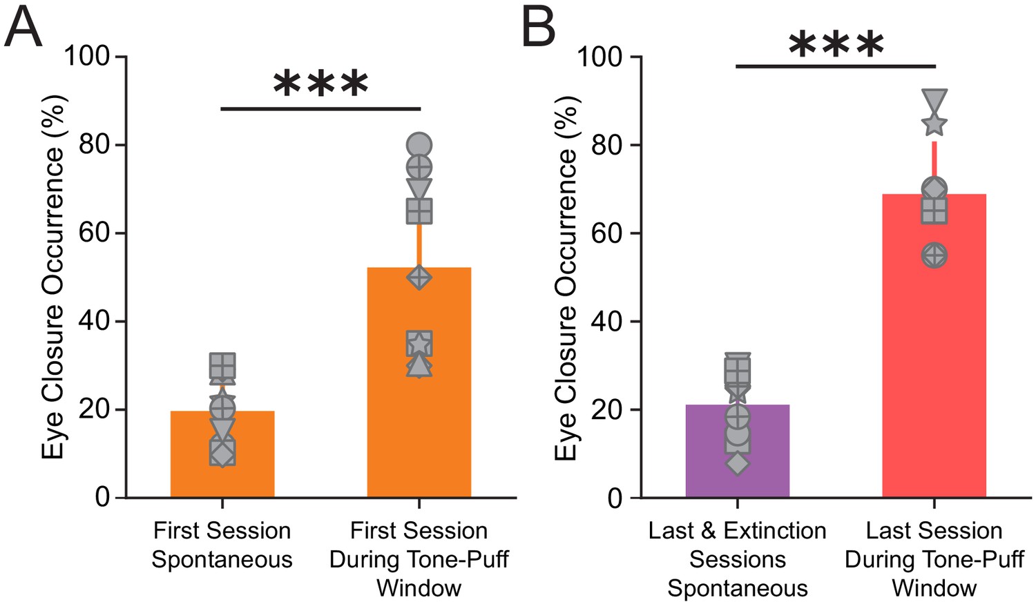
Conditioned vs. spontaneous eye closure responses.
(A) Eye closure occurrence during non-stimulus periods (i.e., spontaneous eye closure occurrence) and conditioned eye closure occurrence during tone-puff window of the first training session, ***p=0.0003, n = 9 mice, Wilcoxon rank-sum test. (B) Spontaneous eye closure occurrence during the non-stimulus periods of the last training and extinction sessions (purple), and conditioned eye closure occurrence during the tone-puff window of the last training session (red), ***p=0.0003, n = 9 mice, Wilcoxon rank-sum test. For all bar plots, error bars are ± s.d.
Figure 2—figure supplement 2
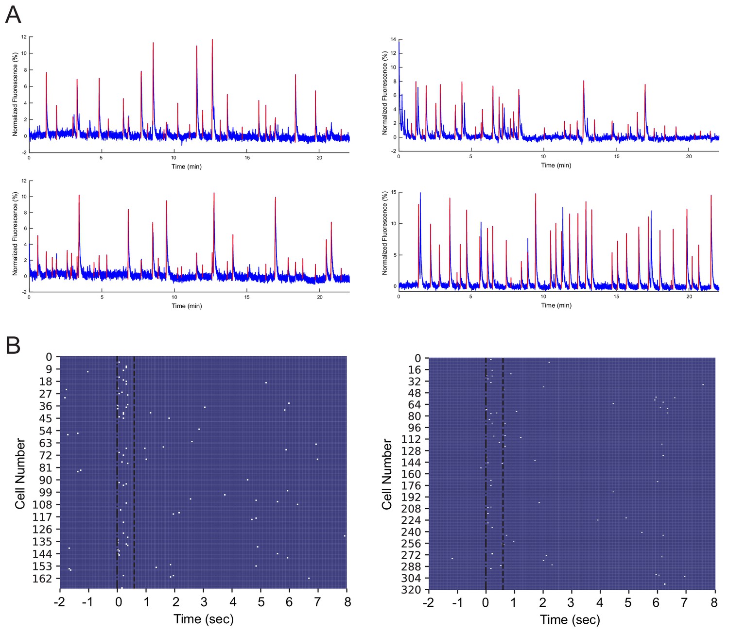
GCaMP6f fluorescence and calcium events in an example recording session.
(A) Representative GCaMP6f fluorescence traces from four neurons. Normalized fluorescence (%) is shown in blue, and the rising phases of identified calcium events are marked in red. (B) Onsets of individual calcium events (marked in white) aligned to tone onset, from simultaneously recorded cells during two representative trials (left and right).
Figure 2—figure supplement 3
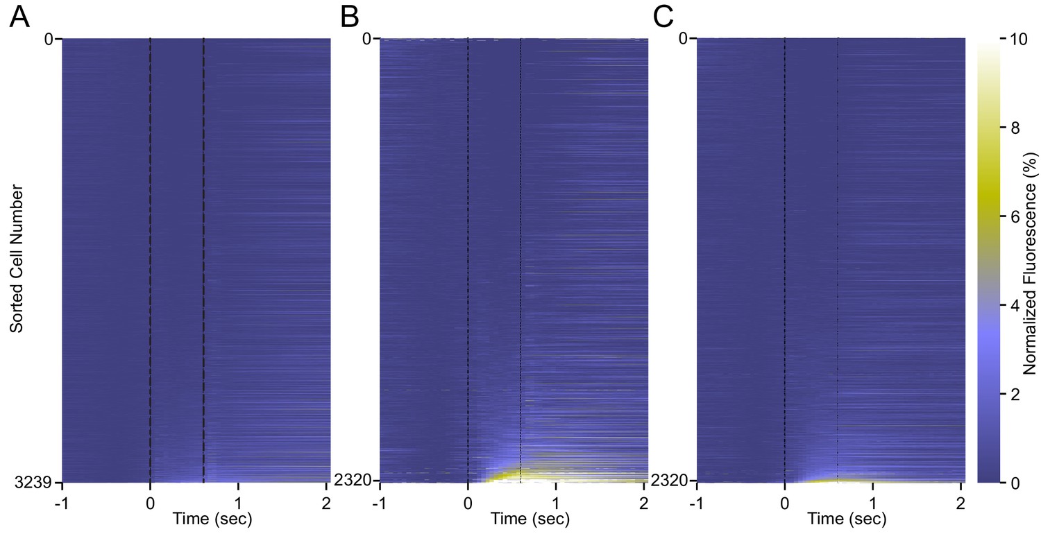
Calcium responses from all neurons recorded in all animals.
Trial-averaged calcium recordings aligned to tone onset for (A) first session, (B) last training session, and (C) extinction session for all cells from all animals. Each plot is sorted by average fluorescence during the tone-puff window for that session.
Figure 2—figure supplement 4
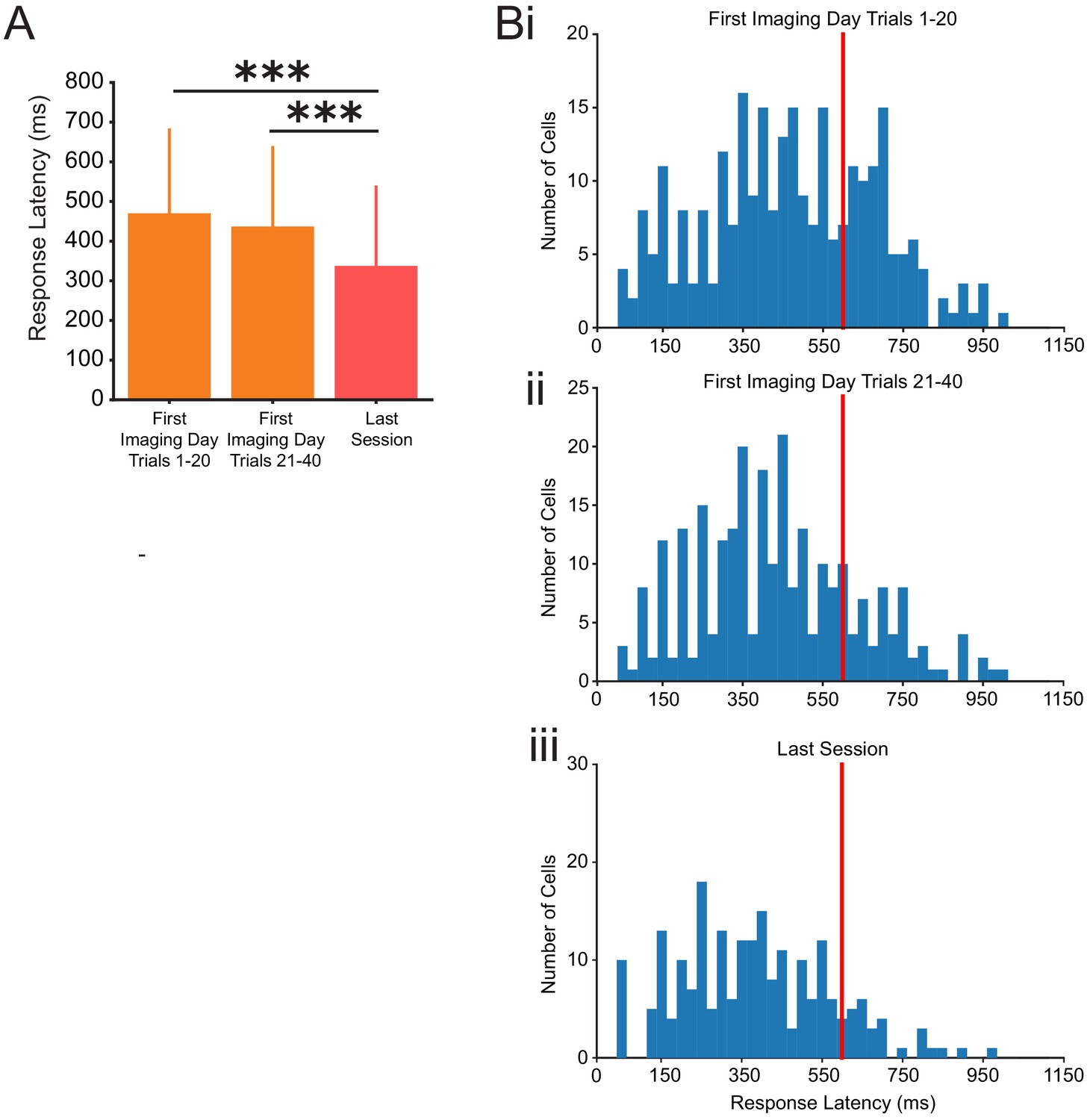
Calcium response latency from all neurons recorded in all animals.
(A) Average latency of calcium event onset following tone onset for responsive cells in trials 1–20 of the first session (orange, left), trials 21–40 of the first session (orange, right), and the last training session (red), one-way ANOVA, post-hoc Tukey test, p=0.15 (between first session trials 1–20 and trials 21–40), ***p=0.001 (between first session trials 1–20 and last session), p=0.001 (between first session trials 21–40 and last session), n = 795 neurons from all three sessions combined. (B) Histogram of response latencies of all responsive neurons from (i) trials 1–20 of the first session, (ii) trials 21–40 of the first session, and (iii) the last session. Puff onset is noted by the red line at 600 ms. For all bar plots, error bars are ± s.d.
Figure 2—figure supplement 5
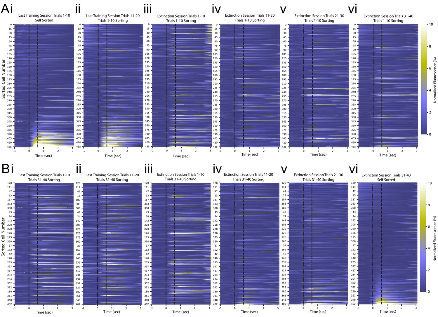
GCaMP6 fluorescence averaged every 10 trials throughout an example recording session.
(A) Trial-averaged calcium recordings aligned to tone onset for (i) trials 1–10 of last training session, (ii) trials 11–20 of last training session, (iii) trials 1–10 of extinction session, (iv) trials 11–20 of extinction session, (v) trials 21–30 of extinction session, and (vi) trials 31–40 of extinction session from the same mouse shown in Figure 2. All plots are sorted by average fluorescence during the tone-puff window of trials 1–10 of the last training session. (B) The same data as shown in (A), sorted by average fluorescence during the tone-puff window of trials 31–40 of the extinction session.
Figure 3
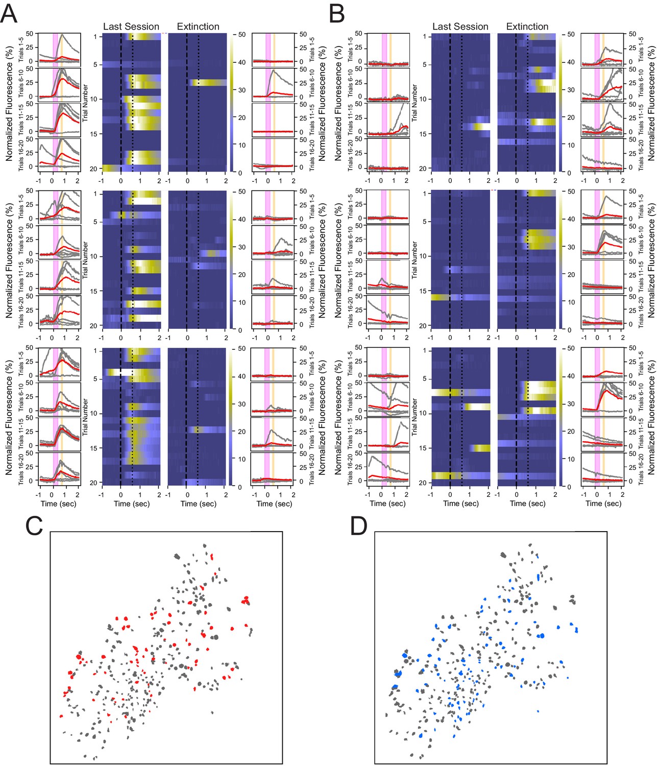
Heterogeneous neuronal responses to the tone during conditioning and extinction learning.
(A) Responses across trials for three neurons that show reliable responding during the last training session, but not during the extinction session, termed CO cells. Outer columns are individual trials shown in gray, and the average of five trials shown in red. The pink box corresponds to the tone, and the orange box corresponds to the puff. Heat maps in the center show each trial for a 3 s time window surrounding the tone and puff presentations. (B) Three neurons that exhibit reliable responding during the extinction session, but not during the last training session, termed EX cells. (C, D) Spatial maps of all neurons from a representative animal during last conditioning training session (C) and extinction session (D), with CO cells in red, EX cells in blue, and all other cells in gray.
Figure 4 with 2 supplements
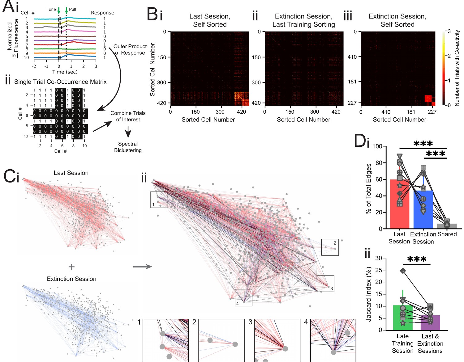
Co-occurrence network analysis during last training session vs. extinction session.
(A) Schematic of method for constructing single-trial co-occurrence matrices. (Ai) A sub-population of cells for one trial that highlights how the response pattern was determined. If a cell exhibited a calcium event (denoted by vertical black line at event onset) during the 1 s window following tone onset, it was assigned a 1. (Aii) The outer product was taken of the vector of responses across the population with itself to generate a single-trial co-occurrence matrix. This is a binary matrix where if the ith and jth cells both exhibit a calcium event during the 1 s window following tone onset there is a 1, but a 0 otherwise. These individual trials can be combined as specific trials of interest and clustered with spectral biclustering to identify neurons with the highest degree of co-activity across those trials. (B) Representative co-occurrence matrices showing clusters of co-active neuron pairs in the last training session (Bi) and the extinction session, with sorting maintained from the last training session matrix (Bii), and re-clustered results based on the matrix during extinction session (Biii). (C) Connectivity maps created from co-occurrence matrices for the last training session (Ci, top), extinction session (Ci, bottom), and overlay (Cii). Edges from the last training session are shown in red, edges from the extinction session are shown in blue, and edges present during both sessions are shown in black. Insets: zoom-ins of four nodes. (Di) Quantification network edges present during the last training session (red), extinction session (blue), or both (gray). t = 0.98, p=0.36 for last vs. extinction sessions, ***t = 7.74, p=5.5e-5 for last session vs. shared and t = 5.73, p=0.0004 for extinction session vs. shared, n = 9 mice, two-tailed paired t-test. (Dii) Percentage of edges that are present in both the first half and last half of the late training session networks (green) vs. the last training session and extinction session networks (purple), ***p=2.48e-8, n = 9 mice, Fisher’s exact test. For all bar plots, error bars are ± s.d.
Figure 4—figure supplement 1
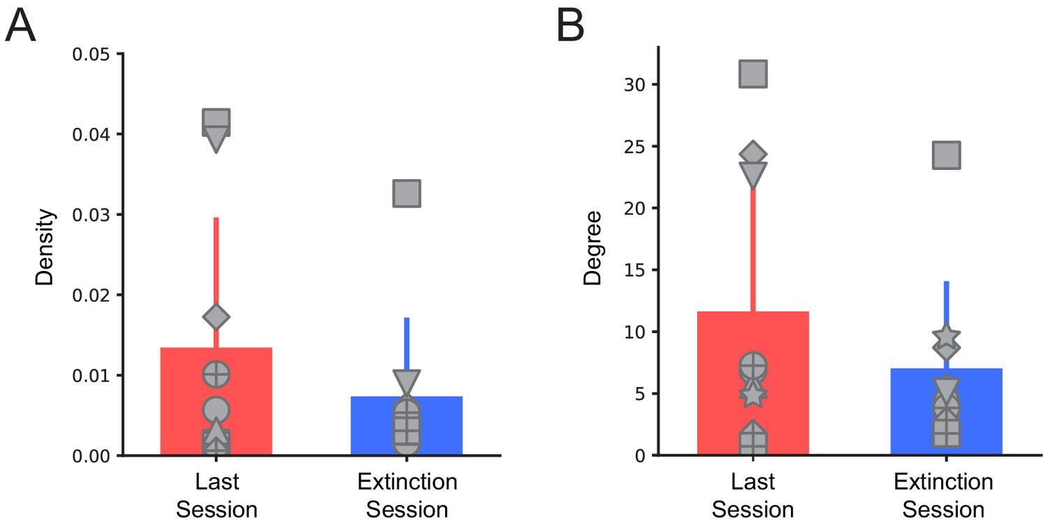
Network degree and density.
(A) Average density and (B) degree of connectivity maps for the last training and extinction sessions across all animals, shown mean + s.d. t = 1.78, p=0.11 for density, t = 1.82, p=0.11 for average degree, two-tailed paired t-test. For all bar plots, error bars are ± s.d.
Figure 4—figure supplement 2
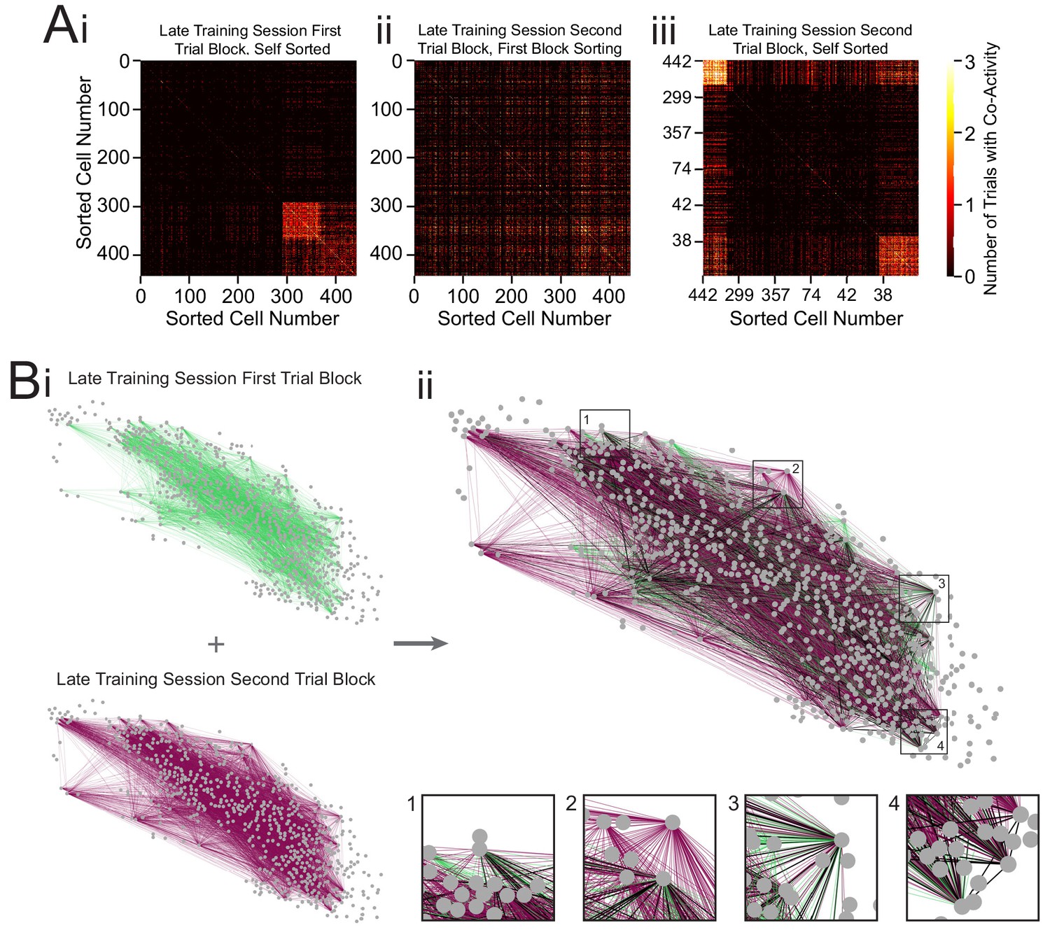
Networks of two separate trial blocks during the late training session.
(A) Representative co-occurrence matrices showing clusters of co-active neuron pairs in the first half of the late training session (Ai) and the second half of the late training session, with sorting maintained from the first half matrix (Aii), and re-clustered results based on the matrix during the second half of the late training session (Aiii). (B) Connectivity maps created from co-occurrence matrices for the first half of the late training session (Bi, top), second half of the late training session (Bi, bottom), and overlay (Bii). Edges from the first half are shown in green, edges from the second half are shown in purple, and edges present during both halves of the late training session are shown in black. Insets: zoom-ins of four nodes.
Author response image 1
Author response image 2
Additional files
-
Supplementary file 1
Marker used in all figures and cell numbers per session for each mouse.
- https://cdn.elifesciences.org/articles/56491/elife-56491-supp1-v3.docx
-
Supplementary file 2
Fisher’s exact test for percentage of responsive cells during first session vs. last training session. n = 7 mice.
- https://cdn.elifesciences.org/articles/56491/elife-56491-supp2-v3.docx
-
Supplementary file 3
Fisher’s exact test for percentage of responsive cells during first session vs. extinction session. n = 7 mice.
- https://cdn.elifesciences.org/articles/56491/elife-56491-supp3-v3.docx
-
Supplementary file 4
Fisher’s exact test for percentage of responsive cells during last training session vs. extinction session. n = 9 mice.
- https://cdn.elifesciences.org/articles/56491/elife-56491-supp4-v3.docx
-
Supplementary file 5
Fisher’s exact test for percentage of common responsive cells during both trial blocks of the late training session vs. last training and extinction sessions. n = 9 mice.
- https://cdn.elifesciences.org/articles/56491/elife-56491-supp5-v3.docx
-
Supplementary file 6
Fisher’s exact test for percentage of shared edges during both trial blocks of the late training session vs. last training and extinction sessions. n = 9 mice.
- https://cdn.elifesciences.org/articles/56491/elife-56491-supp6-v3.docx
-
Transparent reporting form
- https://cdn.elifesciences.org/articles/56491/elife-56491-transrepform-v3.pdf
Download links
A two-part list of links to download the article, or parts of the article, in various formats.
Downloads (link to download the article as PDF)
Open citations (links to open the citations from this article in various online reference manager services)
Cite this article (links to download the citations from this article in formats compatible with various reference manager tools)
Distinct neuronal populations contribute to trace conditioning and extinction learning in the hippocampal CA1
eLife 10:e56491.
https://doi.org/10.7554/eLife.56491


