Structure and dynamics of a nanodisc by integrating NMR, SAXS and SANS experiments with molecular dynamics simulations
- Structural Biology and NMR Laboratory and Linderstrøm-Lang Centre for Protein Science, Department of Biology, University of Copenhagen, Denmark
- Structural Biophysics, X-ray and Neutron Science, Niels Bohr Institute, University of Copenhagen, Denmark
- Department of Chemistry, Aarhus University, Denmark
- Novo Nordisk A/S, Denmark
Figures
Figure 1 with 4 supplements
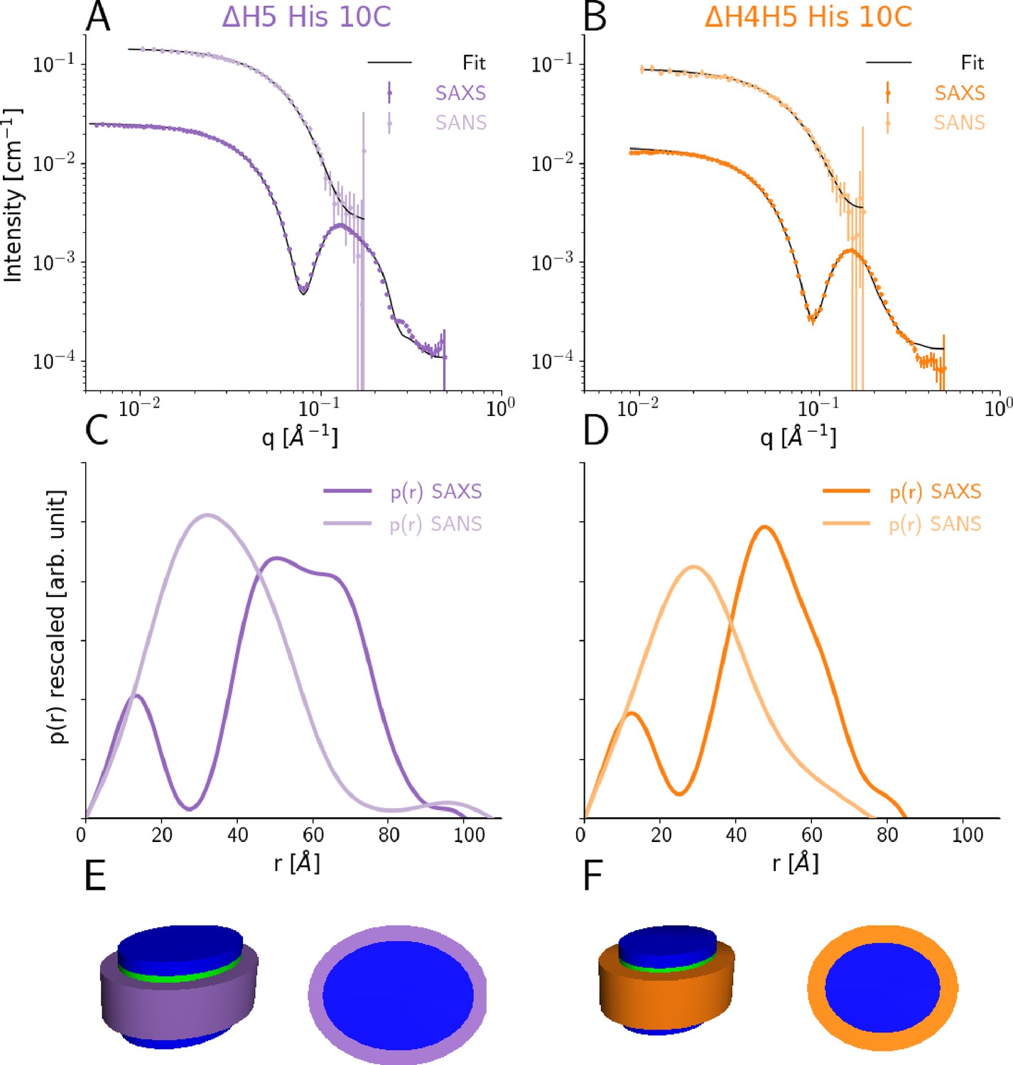
SEC-SAXS and SEC-SANS analysis of nanodiscs.
(A) SEC-SAXS (dark purple) and SEC-SANS (light purple) for ΔH5-DMPC nanodiscs at 10°C. The continuous curve show the model fit corresponding to the geometric nanodisc model shown in E. (B) SEC-SAXS (dark orange) and SEC-SANS (light orange) data for the ΔH4H5-DMPC nanodiscs at 10°C. (C,D) Corresponding pair-distance distribution functions. (E, F) Fitted geometrical models for the respective nanodiscs (drawn to scale relative to one another).
Figure 1—figure supplement 1
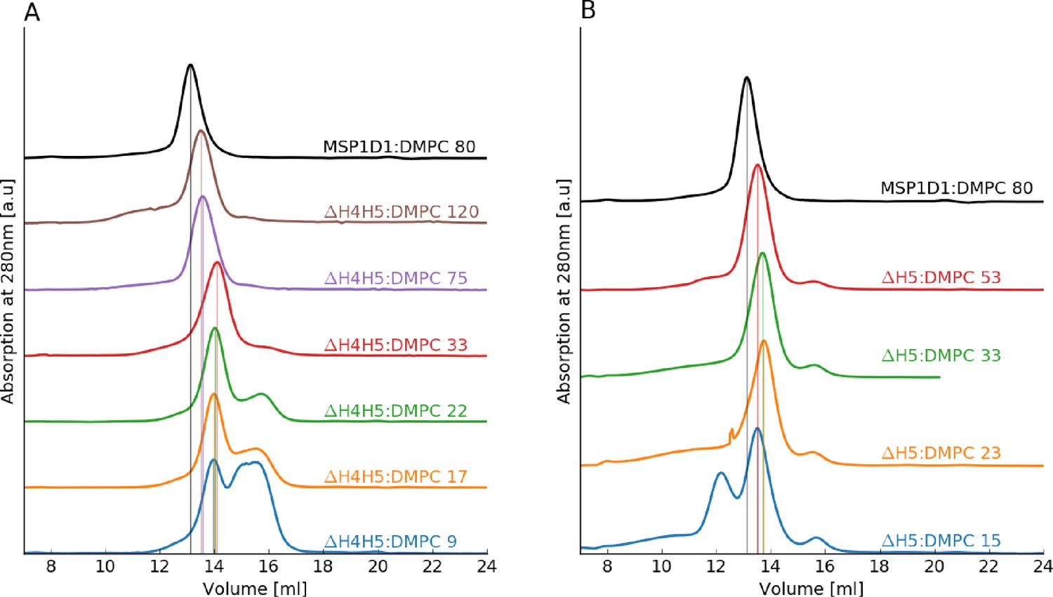
SEC analysis of the reconstitution of ΔH4H5 and ΔH5 nanodiscs with DMPC.
(A) ΔH4H5 with DMPC at variable molar ratios of DMPC to ΔH4H5 with the molar stoichiometry indicated in the plot. (B) ΔH5 with DMPC at variable molar ratios of DMPC to ΔH4H5. In both plots, a reconstitution of MSP1D1:DMPC is inserted as reference (black line). The SEC analysis is performed using a GE Healthcare Life Science Superdex 200 10/300 GL column.
Figure 1—figure supplement 2
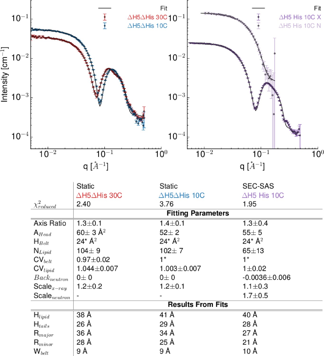
Model-based interpretation of the SAXS/SANS data on DMPC based nanodiscs obtained under different conditions.
Top left) SAXS data from ΔH5ΔHis (I.e. ΔH5 with removed his-tags) obtained at 30°C (red) and 10°C (blue). Experimental data (points) and model fits (full lines). Top right) His-tagged ΔH5-DMPC nanodiscs measured at 10°C with SEC-SAXS (dark violet) and SEC-SANS (light violet). Data were fitted with the analytical model for nanodiscs with elliptical cross-section (see description in main article). Bottom) Table with the parameter values of the shown best model fits for the different samples. In all cases, that is, with/without His-tag and below and above the DMPC melting temperature, we found an axis ratio of the formed discs different from unity (between 1.2 and 1.4). Hence neither the variation of temperature nor the removal of the His-tag affects the overall conclusion that the elliptically-shaped nanodiscs describe the obtained small-angle scattering data.
Figure 1—figure supplement 3
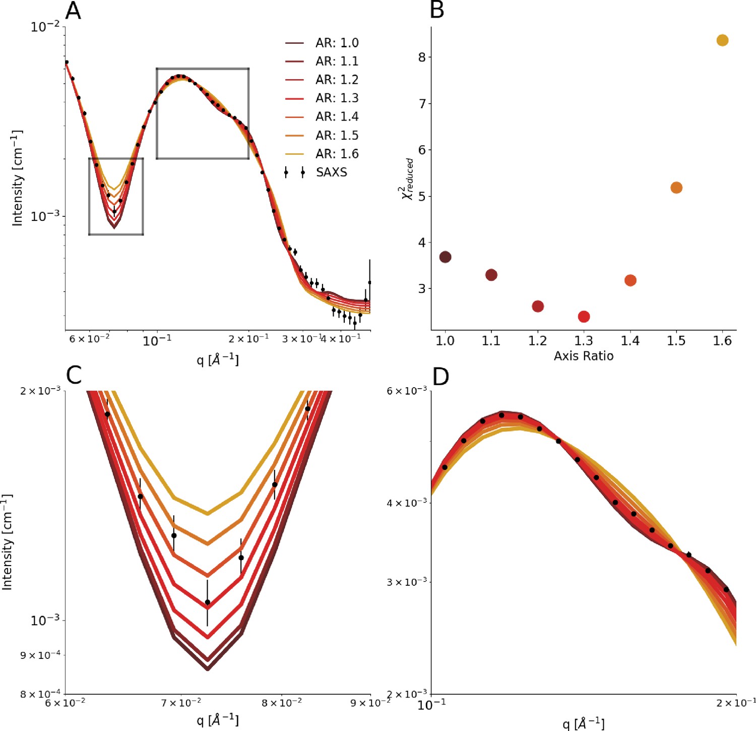
Varying the axis ratio in the model.
We repeated the parameterization of the coarse-grained model by scanning a range of fixed values of the axis ratio and refitted the remaining parameters to optimize the fit. (A) Comparison between experimental SAXS data and those calculated from the model with different values of the axis ratio (AR). (B) Quantification of the agreement between experiment and model. (C and D) show zoom ins on regions highlighted in A.
Figure 1—figure supplement 4
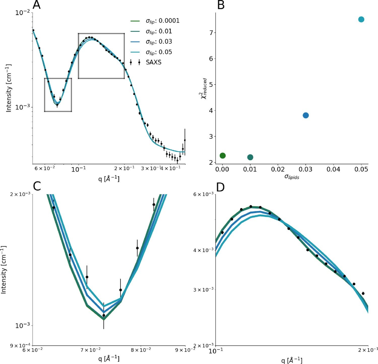
Introducing polydispersity in the model.
We implemented a model for the nanodiscs that included a normally distributed dispersity around the average number of embedded lipids, where the width of the Gaussian was defined by its relative standard deviation in the number of embedded lipids, , and truncated the Gaussian at . An upper hard limit for the number of lipids in the distribution was furthermore defined by the value that yielded circular and hence fully loaded discs. A lower hard limit was defined by the value that yielded discs with axis ratios exceeding 2. (A) Comparison between experimental SAXS data and those calculated from the model with different values of , with representing a monodisperse system. (B) Quantification of the agreement between experiment and model. (C and D) show zoom ins on regions highlighted in A.
Figure 2 with 6 supplements
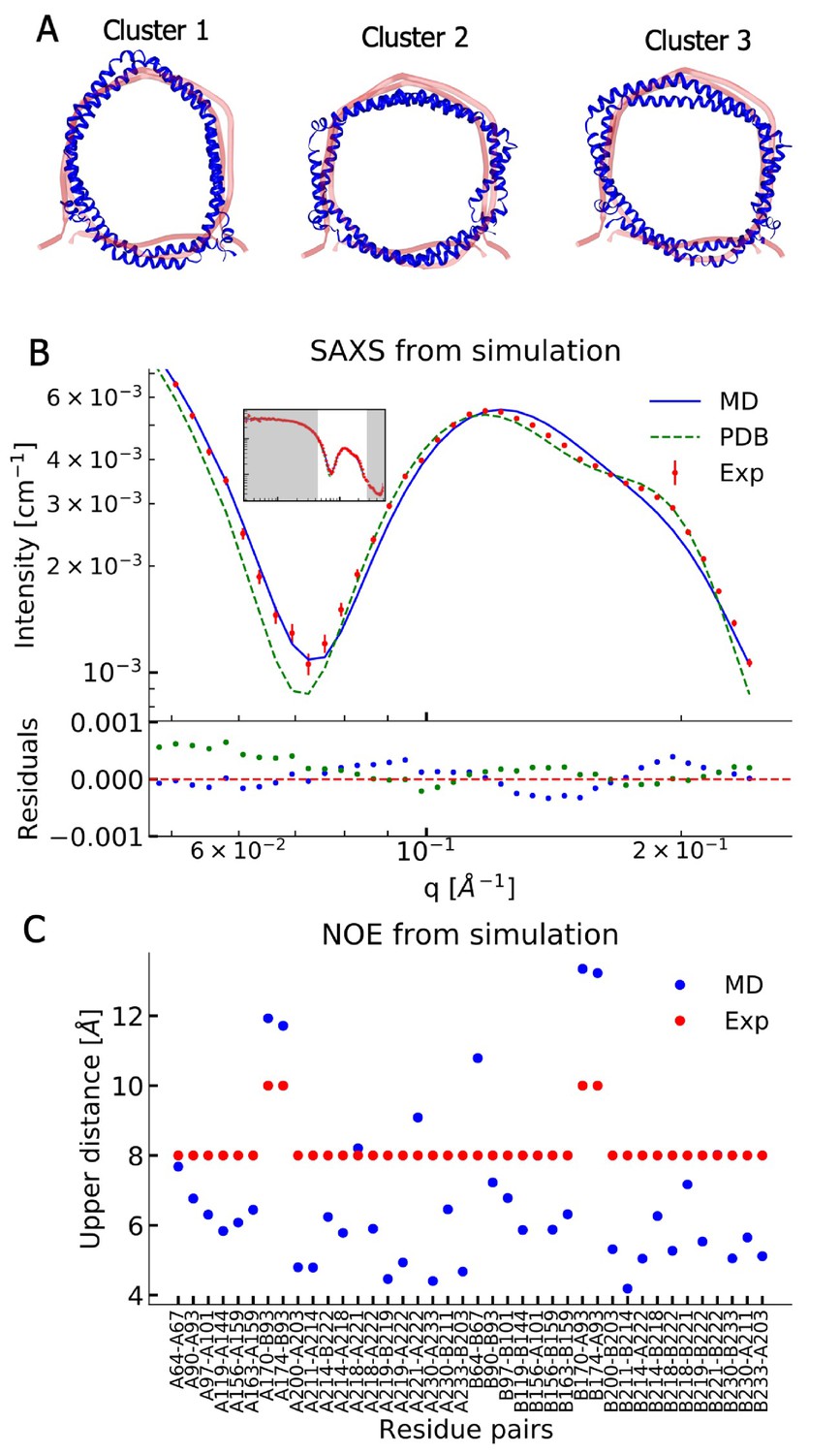
Comparing MD simulations with experiments.
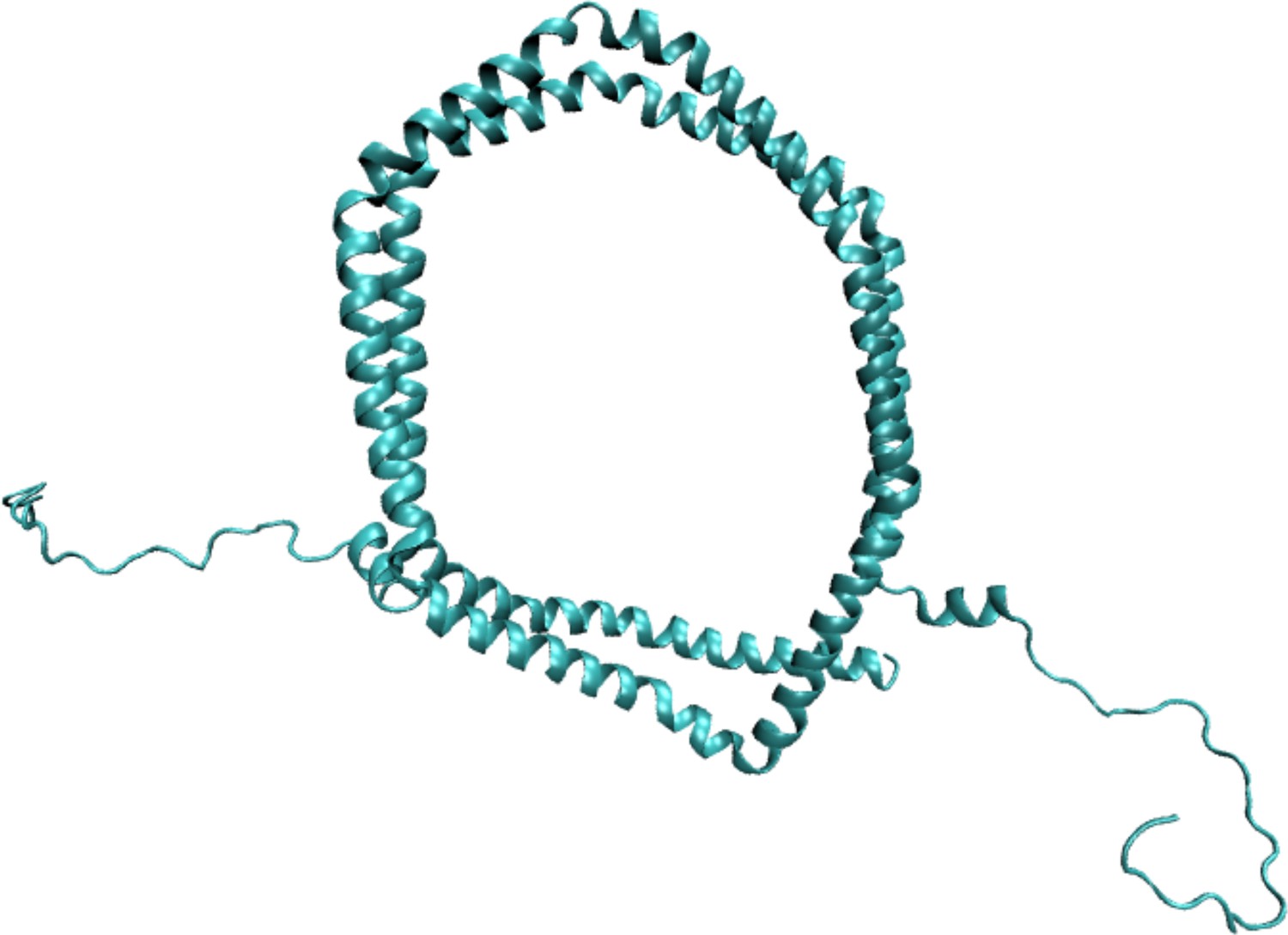
(A) Visualization of the conformational ensemble from the MD simulation by clustering (blue). Only the protein parts of the nanodisc are visualized while the lipids are left out to emphasize the shape. The top three clusters contain 95% of all frames. The previous NMR/EPR-structure is shown for comparison (red). (B) Comparison of experimental standard solution SAXS data (red) and SAXS calculated from the simulation (blue). Green dotted line is the back-calculated SAXS from the integrative NMR/EPR-structure (labelled PDB). Residuals for the calculated SAXS curves are shown below. Only the high q-range is shown as the discrepancy between simulation and experiments are mainly located here (for the entire q-range see Figure 2—figure supplement 1). (C) Comparison of average distances from simulations (blue) to upper-bound distance measurements (red) between methyl NOEs. The labels show the residues which the atoms of the NOEs belong to.
Figure 2—figure supplement 1
Comparing simulations with SAXS data.
This figure is an expanded version of that in the main text, which shows only part of the q-range (marked in white).
Figure 2—figure supplement 2
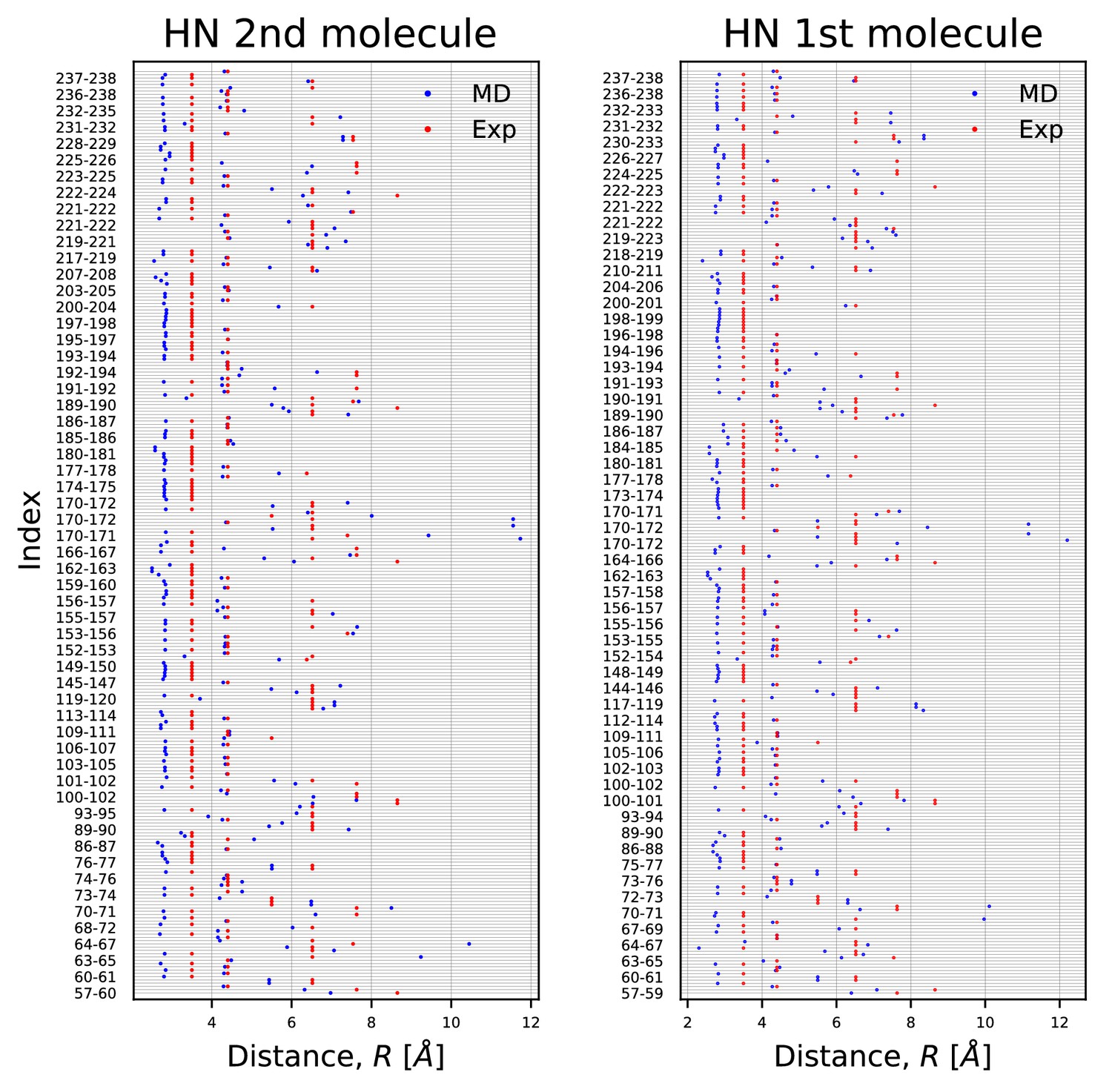
HN-NOE.
Comparison of average distances from simulations (blue) to upper-bound distance measurements (red) between HN-NOEs.
Figure 2—figure supplement 3
Example of a His-tagged nanodisc used for SANS calculations.
Figure 2—figure supplement 4
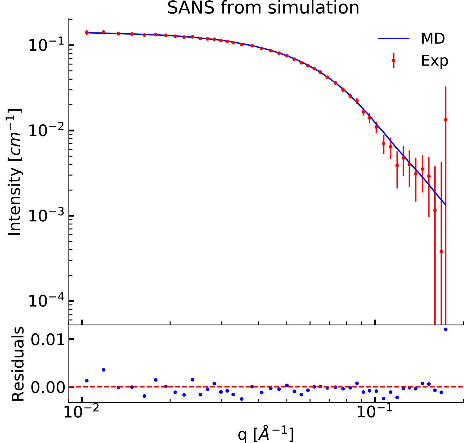
Comparing MD simulations with SANS data.
Figure 2—figure supplement 5
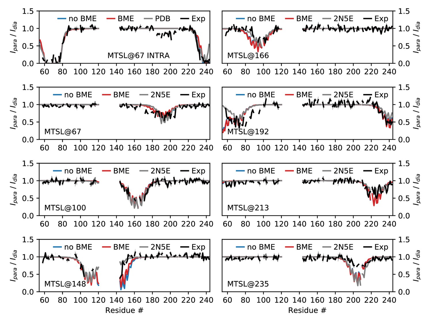
Comparing MD simulations with PRE data.
Each panel corresponds a different probe position as indicated by the labels. We show the experimental values (black), those calculated from the structure determined using these and other data (grey) and our MD simulations both before (blue) and after (red) reweighting. For many probe positions and residues, the values calculated from the PDB structure and our simulations are very similar, so that the colored lines appear hidden beneath the grey line.
Figure 2—figure supplement 6
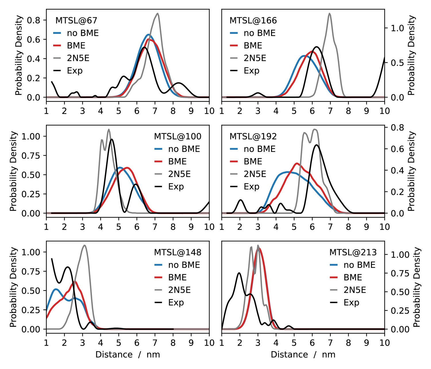
Comparing MD simulations with EPR data.
Each panel corresponds a different probe position as indicated by the labels. We show the distance distributions estimated from the experimental measurements (black), and compare to those calculated from the structure determined using these and other data (grey) and our MD simulations both before (blue) and after (red) reweighting.
Figure 3 with 4 supplements
Integrating simulations and experiments.
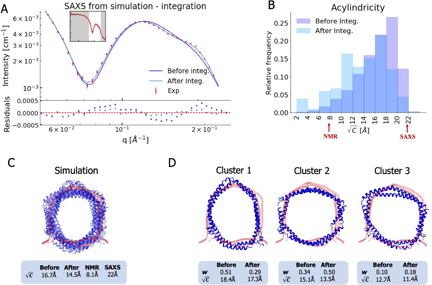
(A) SAXS data calculated from the simulation before and after reweighting the ensemble using experimental data. Only the high q-range is shown as the discrepancy between simulation and experiments are mainly located here (for the entire q-range see Figure 3—figure supplement 1). Agreement with the NOEs before and after integration are likewise shown in Figure 3—figure supplement 2. (B). Histogram of the acylindricity of the simulations () both before integration (dark blue) and after integration (light blue). (C) Visualization of the conformational ensemble showing structures sampled every 100 ns in cartoon representation (blue), the original NMR/EPR structure is shown in rope representation for comparison (red). The table below shows the acylindricity of the entire conformational ensemble before and after integration and compared to the original NMR/EPR (NMR) structure and the SAXS/SANS model fit. (D) Weights and acylindricity of the three main clusters of the MD simulation (blue) before and after integration.
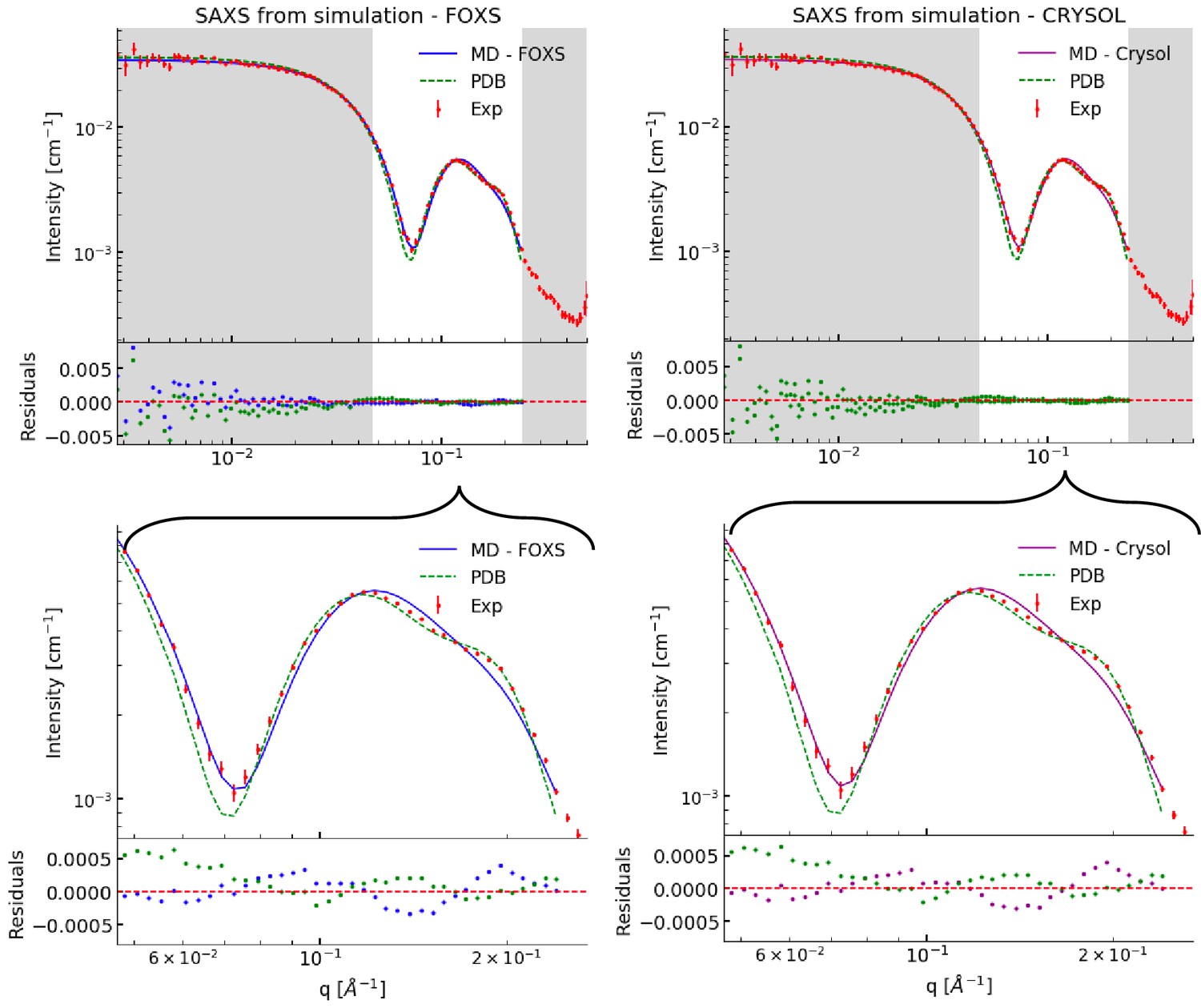
Figure 3—figure supplement 1
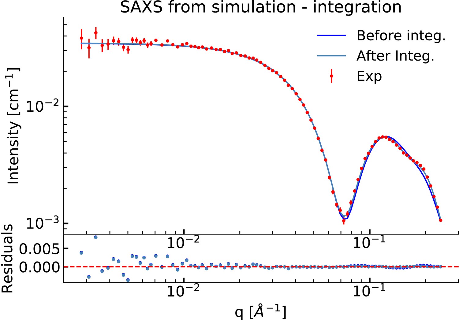
Comparison of the experimental SAXS data from simulation before and after integration.
This figure is an expanded version of that in the main text and shows agreement with the simulation after reweighting. SAXS data were calculated using FOXS.
Figure 3—figure supplement 2
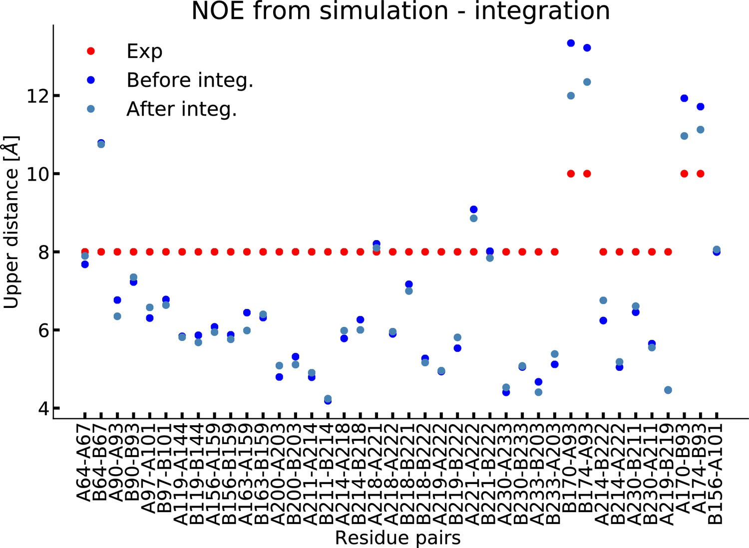
NOEs from simulation before and after reweighting.
Figure 3—figure supplement 3
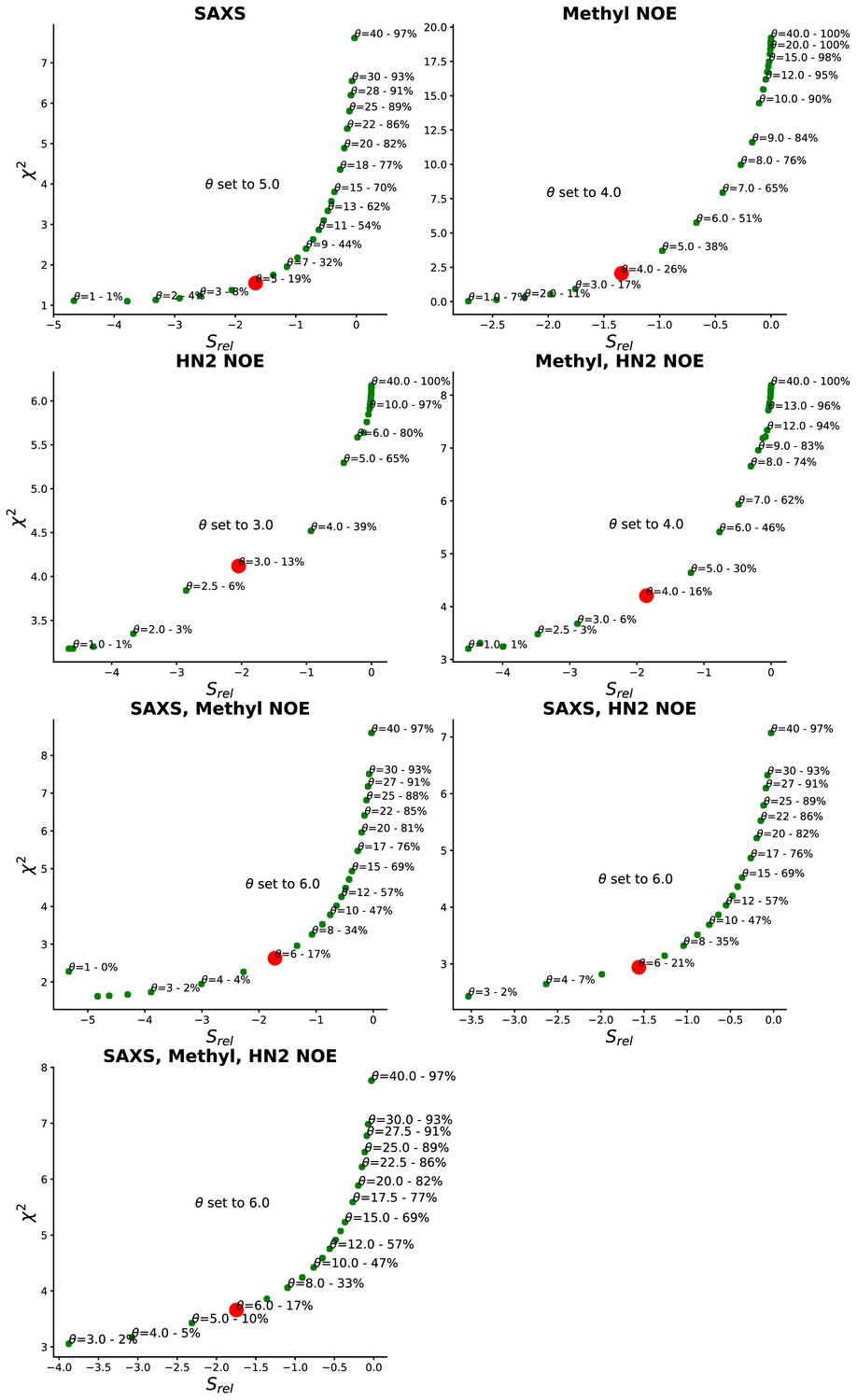
Determination of θ.
θ is a hyperparameter that tunes the balance between fitting the data accurately (low ) and not deviating too much from the prior (low ) thereby avoiding overfitting. It is here determined by plotting vs and selecting a value of θ near the natural kink and at a step where a similar decrease in gives rise to a much lower , indicating that we cannot fit the to the experiments further without a risk of overfitting. The value of θ that produce the given (,) is annotated above the given point together with a measure of the effective number of frames used from the original simulation this gives rise to. Red dot marks the chosen θ.
Figure 3—figure supplement 4
Combining experiments and simulations.
Similar analysis to the main text, but with the methyl- and HN-NOEs integrated individually. As can be seen, the methyl-NOE distances have a larger impact, likely due to the longer distances measured in methyl-NOE whereas the HN-NOEs mainly report on distances between atom pairs of 4 residues or less apart in the sequences and, thus, likely mainly on the helical secondary structure.
Figure 4
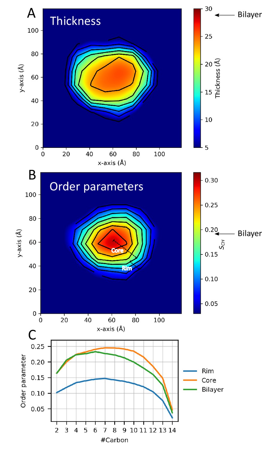
Lipid properties from simulations.
2D plots of the (A) thickness and (B) order parameters averaged over the ensemble and all C-H bonds in the two aliphatic tails of the DMPC lipids in the ΔH5 nanodisc. The core and rim zones are indicated in panel B. Arrows indicate the average value in simulations of a DMPC bilayer. (C) The order parameters as a function of carbon number in the lipid tails in the ΔH5-DMPC disc. The rim zone is defined as all lipids within 10 Å of the MSPs, while the core zone is all the lipids not within 10 Å of the MSPs.
Figure 5
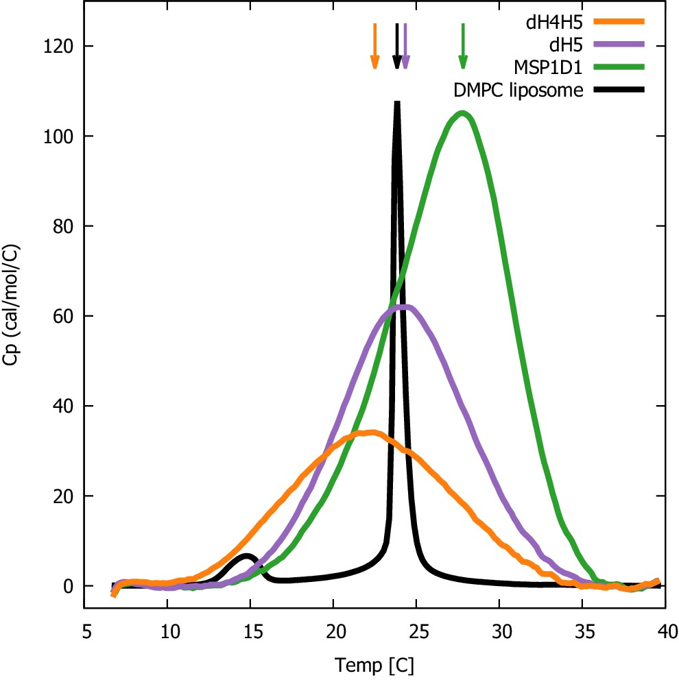
DSC analysis of lipid melting in nanodiscs.
The three DMPC-filled nanodiscs studied, listed by increasing size, are ΔH4H5-DMPC (orange), ΔH5-DMPC (purple) and MSP1D1-DMPC (green). DSC data from plain DMPC-vesicles (black) are shown for comparison. Arrows indicate the temperature with maximal heat capacity. DSC data from the three nanodisc samples are normalized by DMPC concentration, while the data from the DMPC liposome is on an arbitrary scale.
Tables
Table 1
Parameters of the SAXS and SANS model fit.
Left: Parameters for the simultaneous model fits to SEC-SAXS and SEC-SANS of His-tagged nanodiscs (denoted -His) for both ΔH4H5-DMPC and ΔH5-DMPC. Both measurements were obtained at 10°C. Right: Standard solution SAXS measurements of the ΔH5-DMPC nanodisc without His-tags (denoted -ΔHis) obtained at two different temperatures, in the gel phase at 10°C and in the liquid phase at 30°C. * marks parameters kept constant.
| SEC-SAXS+SEC-SANS | SAXS | |||
|---|---|---|---|---|
| ΔH4H5-His | ΔH5-His | ΔH5-ΔHis | ΔH5-ΔHis | |
| T | 10°C | 10°C | 10°C | 30°C |
| χ2reduced | 1.95 | 5.12 | 3.76 | 2.40 |
| Fitting Parameters | ||||
| Axis Ratio | 1.3 ± 0.4 | 1.2 ± 0.2 | 1.4 ± 0.1 | 1.3 ± 0.1 |
| 55 ± 5 Å2 | 54 ± 2 Å2 | 52 ± 2 Å2 | 60 ± 3 | |
| 24* Å2 | 24* Å2 | 24* Å2 | 24* Å2 | |
| 65 ± 13 | 100 ± 14 | 102 ± 7 | 104 ± 9 | |
| 1* | 1* | 1* | 0.97 ± 0.02 | |
| 1.00 ± 0.02 | 1.01 ± 0.01 | 1.003 ± 0.007 | 1.044 ± 0.007 | |
| Scalex–ray | 1.13 ± 0.28 | 1.1 ± 0.2 | 1.2 ± 0.1 | 1.2 ± 0.2 |
| Scaleneutron | 1.7 ± 0.5 | 0.8 ± 0.2 | - | - |
| Results From Fits | ||||
| 40 Å | 41 Å | 41 Å | 38 Å | |
| 28 Å | 28 Å | 29 Å | 26 Å | |
| 27 Å | 32 Å | 34 Å | 36 Å | |
| 21 Å | 27 Å | 25 Å | 28 Å | |
| 10 Å | 9 Å | 9 Å | 9 Å | |
Table 2
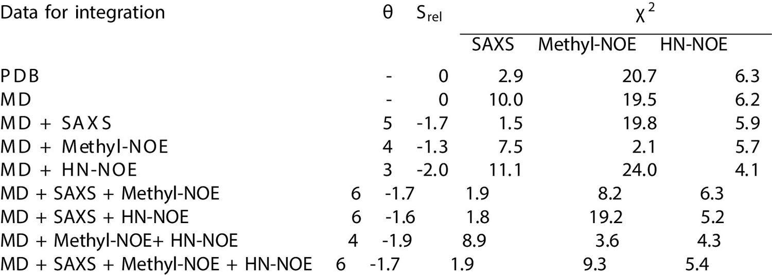
Comparing experiments and simulations.
We quantify agreement between SAXS and NMR NOE experiments by calculating the χ2. The previously determined NMR structure (Bibow et al., 2017) (PDB ID 2N5E) is labelled PDB, the unbiased MD simulation by MD, and simulations reweighted by experiments are labelled by MD and the experiments used in reweighting. is a measure of the amount of reweighting used to fit the data (Bottaro et al., 2018) (see Methods for more details).
| Data for integration | Srel | χ2 | |
|---|---|---|---|
| SAXS | NOE | ||
| PDB | – | 2.9 | 9.5 |
| MD | 0 | 10.0 | 8.2 |
| MD + SAXS | -1.7 | 1.5 | 7.9 |
| MD + NOE | -1.9 | 8.9 | 4.2 |
| MD + SAXS + NOE | -1.7 | 1.9 | 6.0 |
Additional files
Download links
A two-part list of links to download the article, or parts of the article, in various formats.
Downloads (link to download the article as PDF)
Open citations (links to open the citations from this article in various online reference manager services)
Cite this article (links to download the citations from this article in formats compatible with various reference manager tools)
Structure and dynamics of a nanodisc by integrating NMR, SAXS and SANS experiments with molecular dynamics simulations
eLife 9:e56518.
https://doi.org/10.7554/eLife.56518


