Recurrent processes support a cascade of hierarchical decisions
Figures
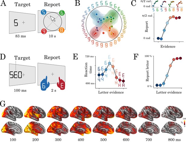
Experimental protocol and behavioral results.
Experiment 1: eight human subjects provided perceptual judgments on variably ambiguous digits briefly flashed at the center of a computer screen (A). Reports were made by clicking on a disk, where (i) the radius and (ii) the angle on the disk indicate (i) subjective visibility and (ii) subjective identity respectively. (B) Distribution (areas) and mean response (dots) location for each color-coded stimulus. (C) Top plots show the same data as B, broken down for each morph set. The x-axis indicates the expected angle given the stimulus pixels (color-coded), hereafter referred to as evidence. The y-axis indicates the angle of the mean response relative to stimulus evidence. The bottom plot shows the same data, grouped across morphs. (D) Experiment 2: seventeen subjects categorized a briefly flashed and parametrically manipulated-morph using a two-alternative forced-choice. Stimulus-response mapping changed on every block. (E) Mean reaction times as a function of categorical evidence (the extent to which the stimulus objectively corresponds to a letter). (F) Mean probability of reporting a letter as a function of categorical evidence. (G) Evoked activity estimated with dSPM and estimated across all trials and all subjects. These data are also displayed in Video 1. Error-bars indicate the standard-error-of-the-mean (SEM) across subjects.
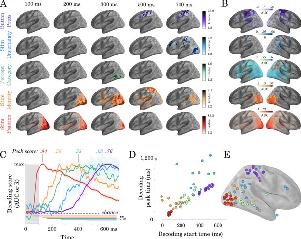
Spatio-temporal hierarchy.
(A) Mass-univariate statistics. Each row plots the average-across-subjects beta coefficients obtained from regression between single-trial evoked activity and each of the five features orthogonally varying in this study. These results are displayed in Video 2. Colors are thresholded based on t-values that exceed an uncorrected p<0.1. We chose this threshold because the perceptual category did not exceed the significance threshold in the univariate tests. (B) Spatial-decoders, consisting of linear models fit across all time sample for each source separately, summarize where each feature can be decoded. Lines indicate significant clusters of decoding scores across subjects cluster-corrected p<0.05. (C) Temporal-decoders, consisting of linear models fit across all MEG channels, for each time sample separately, summarize when each feature can be decoded. To highlight the sequential generation of each representation, decoding scores are normalized by their respective peaks. Additional non-normalized decoding timecourses are available in Figure 2—figure supplements 1 and 2. (D) The peak and the start of temporal decoding plotted for each subject (dot) and for each feature (color). (E) The peak spatial decoding plotted for each subject (dot) and for each feature (color).
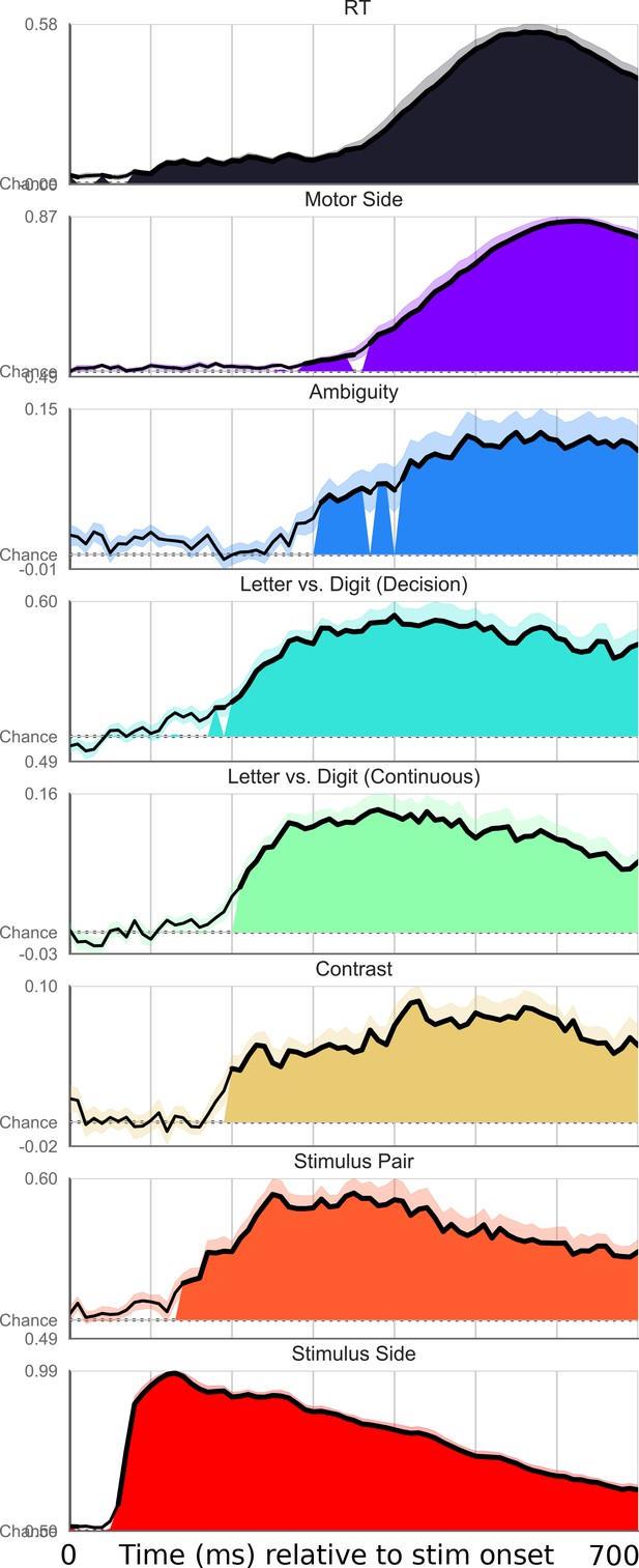
Exhaustive set of results for decoding different features of the stimulus, time-locked to stimulus onset.
Shaded area indicates significant decoding as confirmed with a one-sample temporal cluster test.
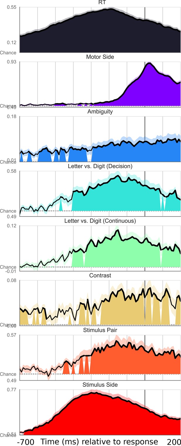
Exhaustive set of results for decoding different features of the stimulus, time-locked to motor onset.
Shaded area indicates significant decoding as confirmed with a one-sample temporal cluster test.
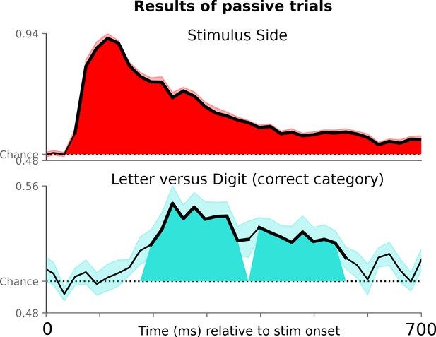
Decoding letter/digit contrast for symbols not presented in the active condition, where subjects viewed the symbols passively and did not have to make a motor response.
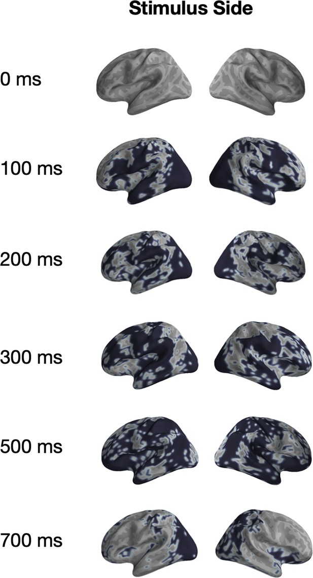
Univariate significance mask for ‘Stimulus Position’.
Localized sources that are contained in a significant (p<0.05) cluster and the specified time-points are highlighted in black.
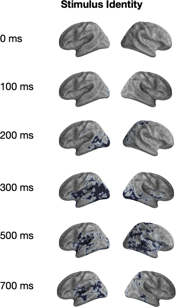
Univariate significance mask for ‘Stimulus Identity’.
Localized sources that are contained in a significant (p<0.05) cluster and the specified time-points are highlighted in black.
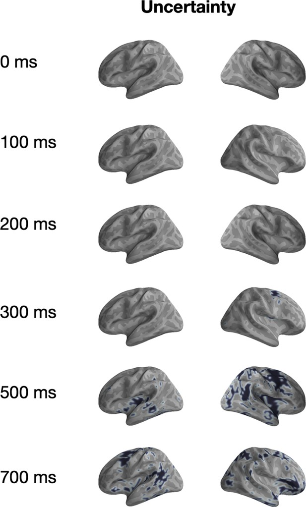
Univariate significance mask for ‘Uncertainty’.
Localized sources that are contained in a significant (p<0.05) cluster and the specified time-points are highlighted in black.
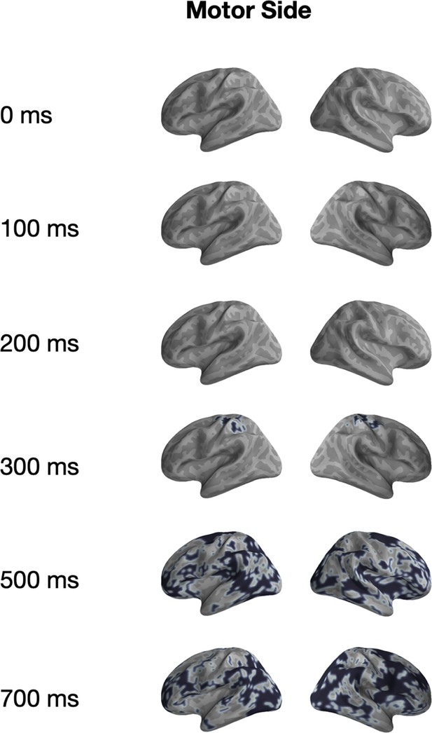
Univariate significance mask for ‘Motor Side’.
Localized sources that are contained in a significant (p<0.05) cluster and the specified time-points are highlighted in black.
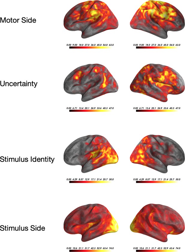
Univariate significance across the four significant features.
Localized sources that are contained in a significant (p<0.05) cluster. Colormap indicates for how many time-points the vertex was included in a cluster.
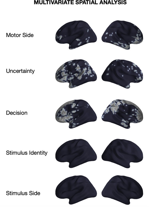
Significance of multivariate tests across the five significant features.
Localized sources that are contained in a significant (p<0.05) cluster in the spatial decoding analysis.
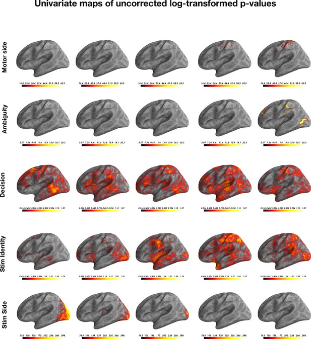
Non-corrected log-transformed (base 10) p-values for the mass univariate tests, plotted for each of the five features.
Note that each feature is has a different color-map threshold.
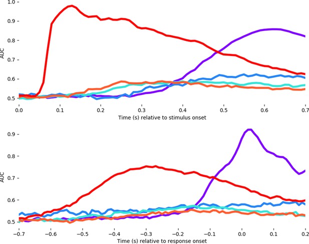
Average decoding timecourses for each of the five features.
Timing is locked to stimulus onset (above) and motor response onset (below). Unlike the analysis of Ambiguity (blue line) in the main test, here we median-split the ambiguity variable to fit a logical regression and thus show the AUC values in comparison to the other features.
Violin plot of decoding accuracy for the five features of interest over time.
Each dot represents a different subject. The shaded area represents the distribution density of the decoding performance scores across subjects. The dashed black line indicates chance decoding performance for that feature.
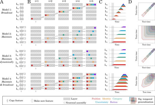
Source and temporal generalization predictions for various neural architectures.
(A) Four increasingly complex neural architectures compatible with the spatial and temporal decoders of Figure 2. For each model (rows), the five layers (L1, L2 … L5) generates new representations. The models differ in their ability to (i) propagate low-level representations across the hierarchy, (ii) maintain information with each layer in a stable or dynamic way. (B) Activations within each layer plotted at five distinct time samples. Dot slots indicate different neural assemblies within the same layer. Colors indicate which feature is linearly represented. For clarity purposes, only effective connections are plotted between different time samples. (C) Summary of the information represented within each layer across time. (D) Expected result for of the temporal generalization analyses, based on the processing dynamics of each model.
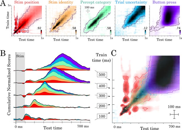
Temporal generalization results.
(A) Temporal generalization for each of the five features orthogonally varying in our study. Color indicate decoding score (white = chance). Contours indicate significant decoding clusters across subjects. (B) Cumulative temporal generalization scores for the temporal decoders trained at 100, 200, 300, 400 and 500 ms, respectively. These decoding scores are normalized by mean decoding peak for clarity purposes. (C) Same data as A but overlaid. For clarity purposes, contours highlight the 25th percentile of decoding performance.
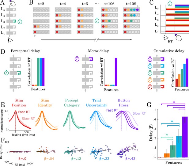
Correlation between TG peaks and reaction times.
(A, B) Recurrent processing at a given processing stage is hypothesized to take a variable amount of time to generate adequate representations. (C) According to this hypothesis, the rise of the corresponding and subsequent representations would correlate with reaction times. (D, left) Predictions when delays are only induced by the perceptual stage of processing. (D, middle) Predictions when delays are only induced by the motor processing processing stage. (D, right) Predictions when delays are induced by all processing stages. (E) TG scores aligned to training time, split into trials within the fastest and slowest reaction-time quantile and averaged across reaction times bins. Dark and light lines indicate the average decoding performance for trials with fastest and slowest reaction times respectively. (F) Each subject (dot) mean peak decoding time (y-axis) as a function of reaction time (x-axis) color-coded from dark (fastest) to light (slowest). The beta coefficients indicate the average delay estimate. (G) The average slope between processing delay and reaction time for each feature. Error-bars indicate the SEM.
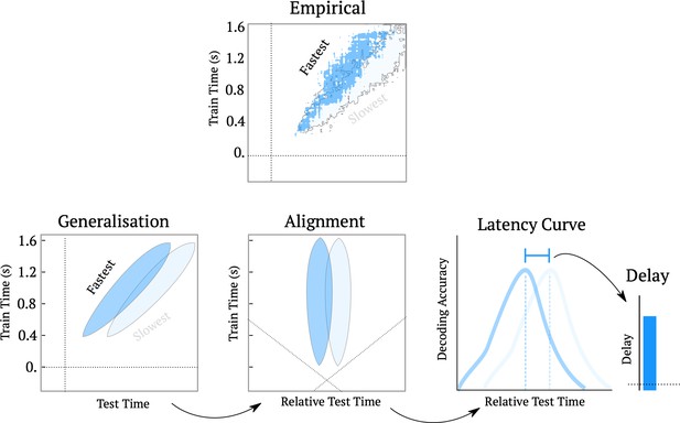
Schematic of the processing delay analysis pipeline.
The top ‘empirical’ figure shows the temporal generalization matrix for decoding ambiguity split into the trials that were responded to the fastest (top 25%) and slowest (bottom 25%). The cartoon below shows the method for estimating latency curves. First we re-align the temporal generalization matrices such that the test-time is shifted relative to the diagonal plane. Then, we average over training times, to yield the latency curve for subsequent analyses.
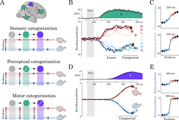
Motor and perceptual decisions.
(A) Hypothesis space for when responses become categorical: during sensory, perceptual or motor processing. (B, top) Time course of decoding the perceptual decision. (B, bottom) Classifier predictions split into different levels of sensory evidence. (C) Averaging probabilities in different time-windows shows the linear-categorical shift in how information is represented. (D, top) Time course of decoding the motor decision. (D, bottom) Splitting classifier predictions into different levels of uncertainty. (E) Different windows of classifier predictions, showing the categorical responses throughout processing.
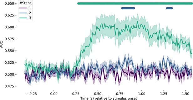
Decoding the distinction between the unambiguous end-points and stimuli at different step distances away.
The purple line corresponds to decoding the difference between unambiguous end-points and one step. A temporal cluster test revealed no significant above-chance decodability. The blue line corresponds to the unambiguous end-points versus two steps. Decoding was significantly above chance from 750 to 900 ms (p<0.001) and again from 1300 to 1400 ms (p=0.007). The teal line corresponds to the unambiguous end-points versus three steps. Decoding was significant from 270 to 1570 ms (p<0.001).
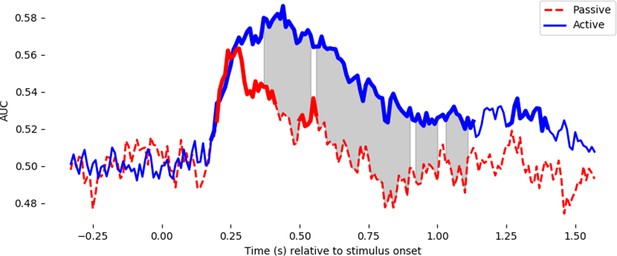
Decoding performance for the letter/digit contrast in active trials requiring a button press (blue line), and passively presented non-ambiguous trials requiring no response (red line).
For the active trials, the classifier is fit with a k-fold cross-validation – training on active trials and testing on active trials. For the passive trials, the classifier is trained on all of the active trials and tested on the 320 passive trials. Note that the actively presented letter/digit stimuli (4, 6 vs H, E) were different from the passively presented ones (9, 8 vs. A, C), thus any significant generalization of neural responses demonstrates a true ‘letter/digit’ percept, which is not specific to particular pixel arrangements. Thicker lines in the decoding timecourses show the timing of significant above-chance decoding for passive trials and active trials separately. Shaded grey areas show when the two timecourses significantly diverge. Both statistical tests used a temporal permutation cluster test and clusters are displayed that are significant at p<0.05.
Videos
Source-localized evoked response averaged over all trials and subjects.
Activity is plot in noise-normalized dSPM units, and shown on an inflated cortical surface (center) as well as a two-dimensional ‘glass brain’ that shows activity averaged over the transverse plane (bottom right).
Temporal decoding results.
For each regressor of interest, the trajectory of normalized decoding accuracy is plot over time. The beta coefficients from the univariate spatio-temporal analysis are plot on the inflated brains, averaged over subjects. The timing of the beta coefficients corresponds to the timing of the normalized decoding accuracy, as shown in the ms counter at the bottom.
Additional files
-
Supplementary file 1
Summary table showing the timing and significance of the results across the five features across the three statistical analyses (temporal decoding, spatial decoding and mass univariate).
pfc corresponds to the p-value after Bonferroni correction across the five features. Average t-value corresponds to the average t-value in the cluster.
- https://cdn.elifesciences.org/articles/56603/elife-56603-supp1-v2.docx
-
Transparent reporting form
- https://cdn.elifesciences.org/articles/56603/elife-56603-transrepform-v2.docx


