A size principle for recruitment of Drosophila leg motor neurons
- Department of Physiology and Biophysics, University of Washington, United States
- Department of Biochemistry and Molecular Biophysics, Department of Neuroscience, Zuckerman Mind Brain Behavior Institute, Columbia University, United States
Figures
Figure 1 with 4 supplements
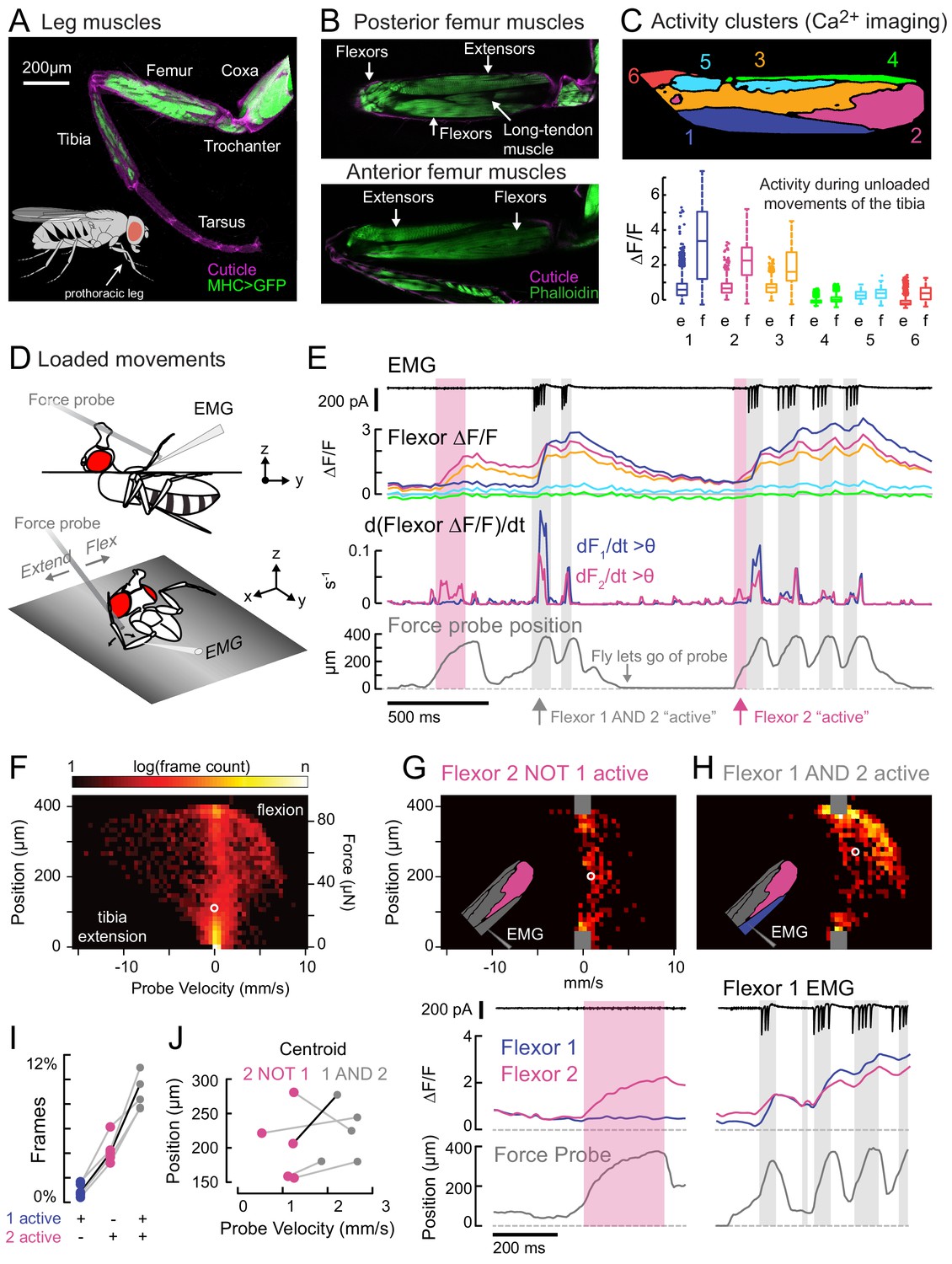
Functional organization and recruitment order among muscles controlling the Drosophila leg.
(A) Muscles of the right prothoracic leg of a female Drosophila (MHC-LexA; 20XLexAop-GFP). (B) Muscles controlling tibia movement in the fly femur. Top and bottom are confocal sections through the femur. Anterior-posterior axis refers to the leg in a standing posture (Soler et al., 2004). (C) Top: K-means clustering of calcium signals (MHC-Gal4;UAS-GCaMP6f) based on correlation of pixel intensities during 180 s of self-generated leg movements in an example fly (unloaded waving, see methods). Bottom: average change in fluorescence for each cluster, in each frame, when the leg is extended (femur-tibia joint >120°, 20772 frames) vs. flexed (<30°, 61,860 frames), n = 5 flies. Flexion activity was consistently higher (p=0.01 for cluster 5, p<10−6 for all other clusters, 2-way ANOVA, Tukey-Kramer correction). (D) Schematic of the experimental setup. The fly is fixed in a holder so that it can pull on a calibrated force probe with the tibia while calcium signals are recorded from muscles in the femur. (E) Calcium activity in tibia muscles while the fly pulls on the force probe (bottom trace). Cluster six was obscured by the probe and not included. The middle row shows the smoothed, rectified derivative of the cluster fluorescence (dFi/dt) for the two brightest clusters (1 and 2), which we refer to as Flexors. Highlighted periods indicate that both Flexors 1 and 2 are active simultaneously (gray, dF/dt > 0.005), or that Flexor 2 alone is active (magenta). (F) 2D histogram of probe position and velocity, for all frames (n = 13,504) for a representative fly. The probe was often stationary (velocity = 0), either because the fly let go of the probe (F = 0), or because the fly pulled the probe as far as it could (F ~ 85 µN), reflected by the hotspots in the 2D histogram. In F–H), the white circles indicate the centroids of the distributions. (G) Top - 2D histogram of probe position vs. velocity when Flexor 2 fluorescence increased, but not Flexor 1 (n = 637 frames, same fly as F). Gray squares indicate hotspots in F), which are excluded here. Color scaled to log(50 frames). Bottom – example of instance in which Flexor 2 alone is active (magenta shading). (H) Top - Same as G), when Flexor 1 AND 2 fluorescence increased simultaneously (n = 1449 frames). Bottom – gray shading indicates instances of activity in both Flexors 1 and 2. (I) Fraction of total frames for each fly in which both Flexor 1 and 2 fluorescence increased (gray), Flexor 2 alone increased (magenta), or Flexor 1 alone increased. Number of frames for each of five flies: 32,916, 13,504, 37,136, 37,136, 24,476. (J) Shift in the centroid of the 2D histogram when Flexor 1 fluorescence is increasing along with Flexor 2 fluorescence (gray), compared to when Flexor 2 fluorescence alone is increasing (p<0.01, Wilcoxon rank sum test). Black line indicates example cell in G) and H).
Figure 1—figure supplement 1
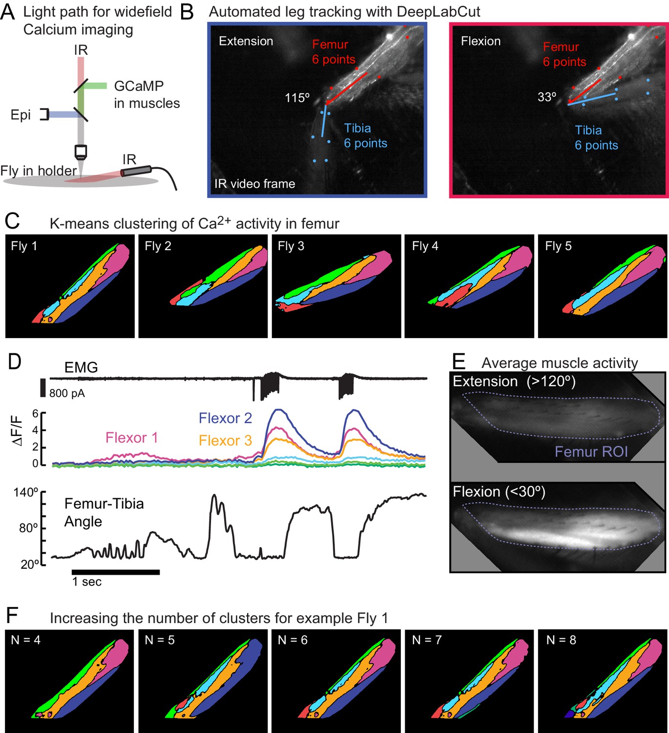
Wide-field calcium imaging of muscles in the femur.
(A) Schematic of light path for widefield calcium imaging of femur muscles. Infrared illumination is used to track leg movement. GCaMP emission is reflected by a longpass dichroic mirror to a second camera. (B) Tracking the femur and tibia with DeepLabCut. A network was trained to detect six points on the femur and six points on the tibia in the IR illuminated videos of the leg. We calculated the center of the tibia from the six detected points. The elliptical arc of the centroid across frames allowed us to estimate the angle of elevation of the tibia relative to the plane of the metal holder (black background). (C) K-means clustering of GCaMP activity in muscle fibers during unloaded movements of the tibia. Clusters were similar across five flies, including the ventral distal cluster 1, the proximal cluster 2, the more dorsal cluster 3, and a thin dorsal cluster 4. Clusters 5 and 6 were more variable in shape and location. (D) Example epoch from Fly one showing the femur-tibia angle and the fluorescence of each cluster. (E) Averaged fluorescence across all frames in which the tibia was extended (top) vs. flexed (bottom), for Fly 1, normalized to the maximum ΔF/F. Note the lack of signal during extension. (F) K-means clustering with different numbers of clusters for Fly 1, shown in Figure 1. With fewer than five clusters, the proximal cluster tended to be much larger, incorporating much of the region labeled as cluster 3. With more than six clusters, the smallest and least modulated clusters tended to divide, not providing any further information. When k = 6, pixels in the extension region clustered together, but we did not see large increases in fluorescence with extension (Figure 1).
Figure 1—figure supplement 2
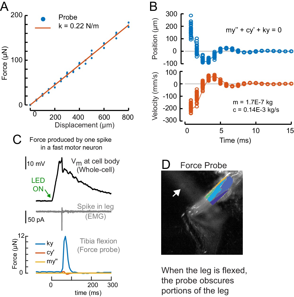
Calibration of the force probe dynamic properties.
(A) The force probe tip was positioned over an analytical balance, and the base of the force probe was displaced. The weight (force) at each displacement is shown in blue, the linear fit is shown in red. The slope of the line is the spring constant, k = 0.2234 N/m. (B) To measure the effective mass and drag constant of the probe in saline, we flicked the force probe by displacing the tip with a glass hook until it lost contact and snapped back to rest. In blue is the displacement in each frame for 16 different flicks. In orange is the velocity. We used the ode45 solver in Matlab to fit the mass (m = 0.17 mg) and drag coefficient (c = 0.14E-3 kg/s). (C) Using the dynamical parameters from b, we calculated the portion of the force due to elastic properties of the force probe (blue), drag (red), and inertia (yellow). Here, a single spike evoked optogenetically in a fast motor neuron produced a small movement of the probe (as in Figure 4A, Video 2). In Figure 4D–F, we calculated force by including drag and inertia, but in other figures we report leg displacement and the approximation of force, assuming that drag and inertia are negligible. (D) The probe obscured the distal leg during spontaneous movements, so we limited the ROI for clustering to the proximal leg.
Figure 1—figure supplement 3
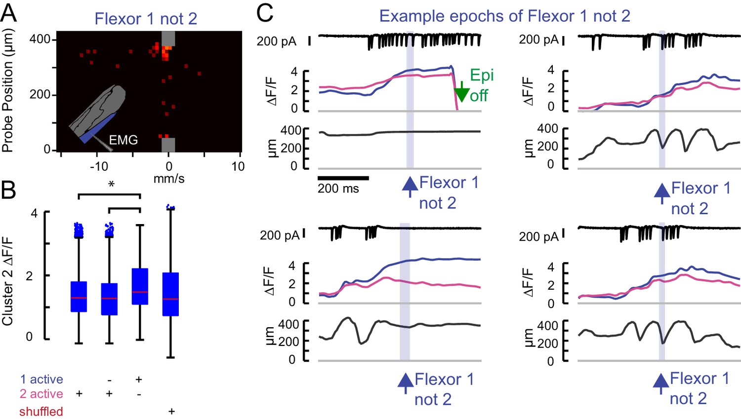
Flexor 2 signal is high whenever Flexor 1 is active.
(A) The force probe histogram for frames when only Flexor 1 was active, scaled according to Figure 1H. (B) Flexor 2 ΔF/F for all frames across N = 5 flies in which 1) Flexor 2 is activating (21962 frames); 2) Flexor 2 alone is activating (6686 frames); 3) when Flexor 1 alone is active (1805 frames); 4) random values of cluster 2 ΔF/F (1805 values). The mean Flexor 2 ΔF/F is higher when Flexor 1 alone is active than when Flexor 2 is active (asterisk, p<10–8, 2-way ANOVA, Tukey-Kramer correction for multiple comparisons), indicating that Flexor 2 is also likely contracting even though ΔF/F is not increasing. (C) Example epochs in which the derivative of Flexor 1 fluorescence, but not Flexor 2 (blue shading) is positive. These epochs make clear that these periods arise when Flexor 2 and 1 are active and contracting together (Flexor 2 ΔF/F high as in Figure 1H), but the derivative of Flexor 2 ΔF/F is either negative or simply not large. The first example occurs near the end of a trial, when the LED was turned off (green arrow).
Figure 1—figure supplement 4
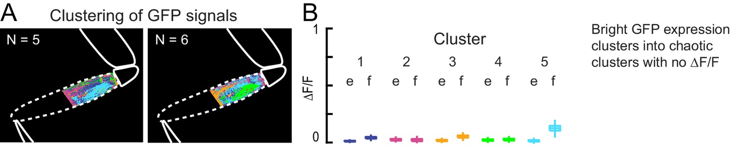
GFP control for k-means clustering of calcium activity.
(A) K-means clustering of GFP expression in muscles during spontaneous movements. Clusters were noisy, interleaved and dispersed. In this case, the fly pulled on the probe and the clusters are superimposed over the image of the fly leg. (B) Changes in fluorescence of clusters calculated from videos of GFP expression during spontaneous movements. GFP expression was bright (as shown in Figure 1A), but did not change with movements.
Figure 2 with 1 supplement
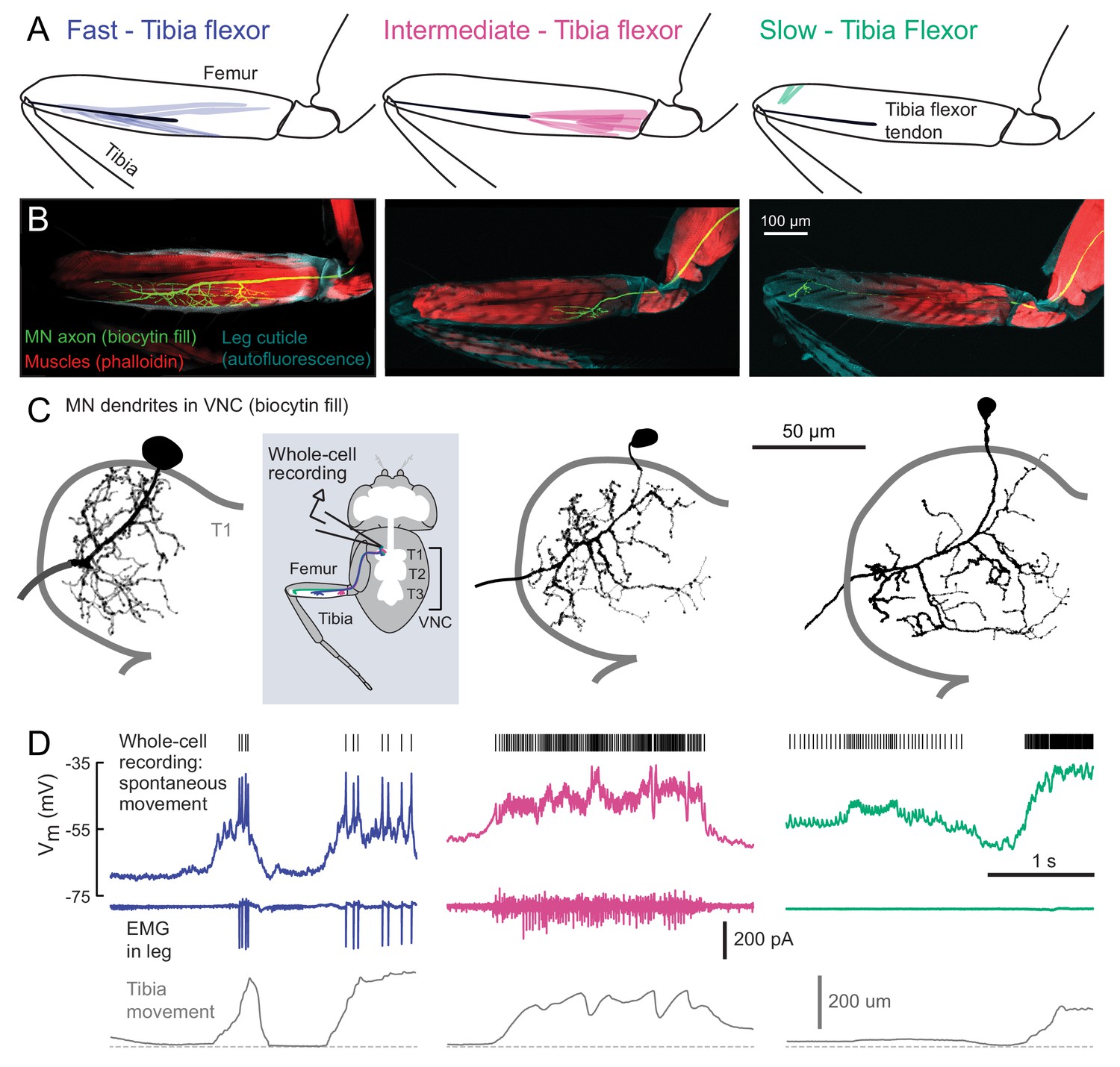
Motor neurons controlling tibia flexion.
(A) Schematic of the muscle fibers innervated by motor neurons labeled by the following Gal4 lines: left: R81A07-Gal4, center: R22A08-Gal4, and right: R35C09-Gal4. (B) Biocytin fills of leg motor neurons from whole-cell patch clamp recordings, labeled in fixed tissue with strepavidin-Alexa-568 (green), counter stained with phalloidin-Alexa-633 (red) labeling actin in muscles, and autofluorescence of the cuticle (cyan). (C) Images of biocytin fills in the VNC following whole-cell patch recordings (schematic). Prothoracic neuromere is outlined. Cells were traced and ‘filled’ with the simple neurite tracer plugin in Fiji. (D) Example recordings from each motor neuron type during spontaneous tibia movement: whole-cell current clamp recordings with detected spike times above (top row, corrected for a liquid junction potential of −13 mV), EMG recordings (middle), and tibia movement (force probe position; bottom). We often observed EMG events from the fast and intermediate neurons. We did not observe EMG events associated with slow neuron firing, though we often observed flexion of the tibia without seeing EMG activity, as seen here.
Figure 2—figure supplement 1
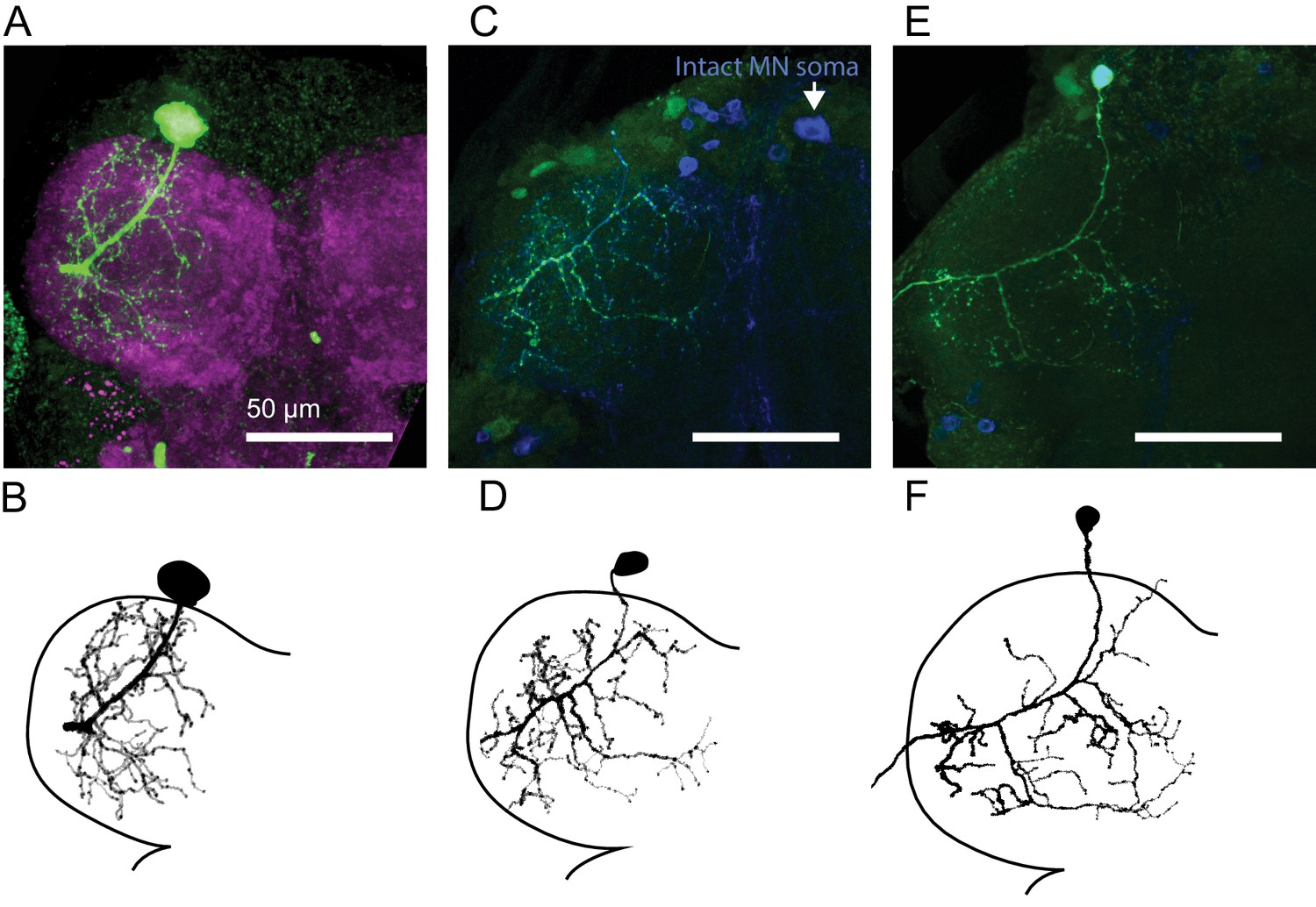
Central anatomy of flexor motor neurons.
(A) Maximum intensity projections of fast flexor motor neuron fill (green, neurobiotin). In magenta is the neuropil (nc82). (B) Traced neuron from A), using the simple neurite tracer plugin in FIJI. Also shown in Figure 2C. (C) Maximum intensity projections of intermediate flexor motor neuron fill (green, neurobiotin). In blue is GFP expression driven by R22A08-Gal4. Note, the cell body of the filled neuron was ripped off, but the motor neuron cell body on the contralateral side remains. (D) Traced neuron from C, as shown in Figure 2C. (E) Maximum intensity projections of slow flexor motor neuron fill (green, neurobiotin). In blue is GFP expression driven by R35C09-Gal4. (F) Traced neuron from E), as shown in Figure 2C.
Figure 3
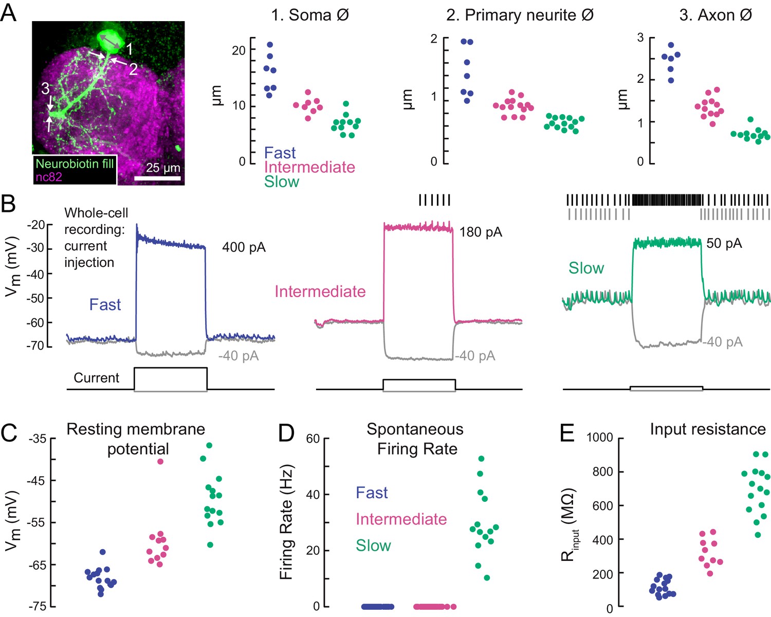
A gradient of intrinsic properties among tibia flexor motor neurons.
(A) Left) Maximum intensity projection of a Neurobiotin fill (green) of the fast tibia flexor motor neuron, with nc82 counterstain. Right) Diameters of identified neuron 1) somas, 2) primary neurites, and 3) axons (p<0.01, 2-way ANOVA, Tukey-Kramer correction for multiple comparisons). (B) Example traces showing voltage responses to current injection in whole-cell recordings from each motor neuron type. (C) Average resting membrane potential for fast (n = 15), intermediate (n = 11), and slow tibia flexor motor neurons (n = 14) (p<0.001, 2-way ANOVA, Tukey-Kramer correction for multiple comparisons). (D) Average spontaneous firing rate in fast (n = 15), intermediate (n = 11), and slow neurons (n = 14) (p<10−5). (E) Input resistance in fast (n = 15), intermediate (n = 11), and slow neurons (n = 14) (p<0.001, 2-way ANOVA, Tukey-Kramer correction for multiple comparisons). All intrinsic properties in C-E) were calculated from periods when the fly was not moving.
Figure 4 with 1 supplement
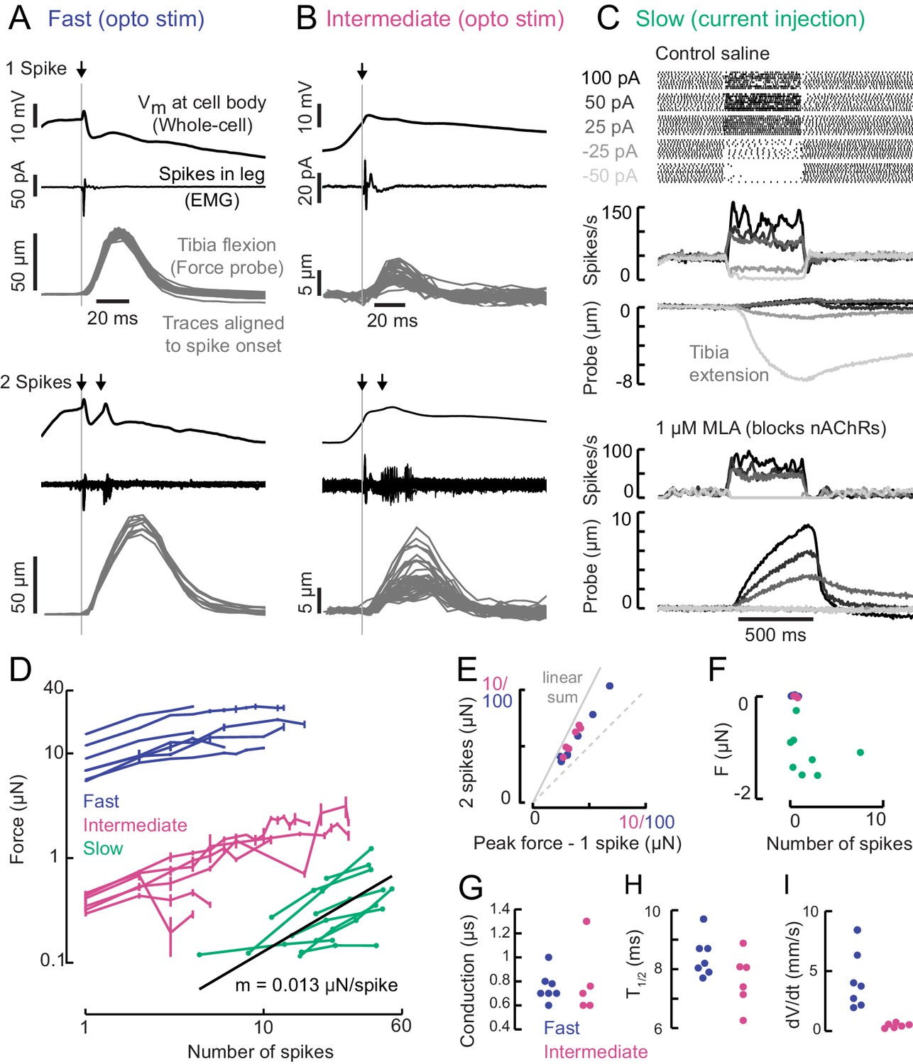
A gradient of force production among tibia flexor motor neurons.
(A) Optogenetic activation of a fast flexor motor neuron expressing CsChrimson (50 ms flash from a 625 nm LED,~2 mW/mm2). Traces show average membrane potential for trials with one (top) and two (bottom) spikes, the average EMG (top) or overlaid EMGs (bottom), and the resulting tibia movement for each trial (50 µm = 11 µN). The jitter in the force probe movement traces results from variability of when a spike occurs relative to the video exposure (170 fps). (B) Same as A for an example intermediate flexor motor neuron. (C) Tibia movement resulting from current injection in a slow flexor motor neuron. Top: spike rasters from an example cell during current injection. Firing rates are shown below, color coded according to current injection value, followed by the baseline subtracted average movement of the probe (5 µm = 1.1 µN). Bottom: spike rates and probe movement in the presence of the cholinergic antagonist MLA (1 µM), which reduces excitatory synaptic input to the motor neuron. (D) Peak average force vs. number of spikes for fast (blue), intermediate (magenta), and slow (green) motor neurons. The number of spikes in slow neurons is computed as the average number of spikes during positive current injection steps minus the baseline firing rate; that is, the number of additional spikes above baseline. The black line is a linear fit to the slow motor neuron data points, with the slope indicated below. (E) Peak probe displacement for 2 spikes vs. one spike in fast (blue) and intermediate motor neurons (magenta). (F) Summary data showing that zero spikes in fast (n = 7) and intermediate neurons (n = 6) does not cause probe movement, but that hyperpolarization in slow motor neurons (n = 9) causes the fly to let go of the probe, that is, decreases the applied force. The number of spikes (x-axis) is computed as the average number of spikes per trial during the hyperpolarization.(G) Delay between a spike in the cell body and the EMG spike (conduction delay). Note there may be a delay from the spike initiation zone to the cell body that is not captured (n = 5 intermediate cells), p=0.6, Wilcoxon rank sum test. (H) Time to half maximal probe displacement for fast (blue) and intermediate cells (magenta), p=0.2, rank sum test. (I) Estimates of the maximum velocity of tibia movement in each fast (blue) and intermediate motor neuron (magenta), p=0.0012, rank sum test. A line was fit to the rising phase of probe points aligned to single spikes as in B) and D).
Figure 4—figure supplement 1
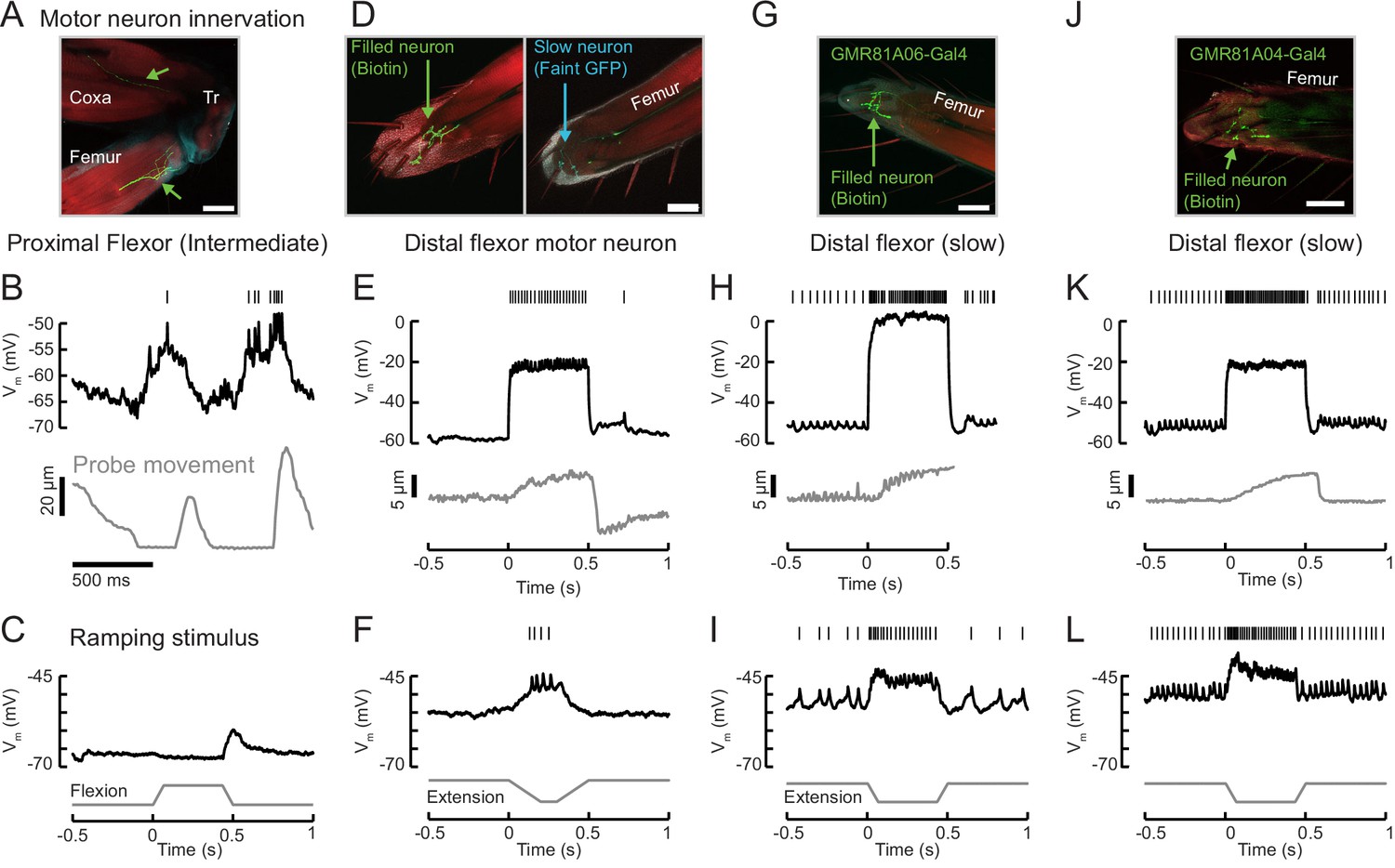
Example recordings from other tibia flexor neurons.
(A) Confocal image of an intermediate flexor motor neuron axon (neurobiotin fill is shown in green; red is phalloidin) from UAS-GFP;R81A06-Gal4. The filled neuron targets the proximal femur. Scale bar is 50 µm. The axon appears to target different fibers than the intermediate neuron in R22A08-Gal4. (B) Membrane potential, spikes, and probe movement during spontaneous movements. Membrane potential reflects and slightly precedes flexion events, and spikes occur at low forces. (C) Single trial example of sensory feedback. The neuron rests at −67 mV. Passive flexion of the leg (60 μm = 8°) hyperpolarizes the intermediate neuron in R81A06-Gal4. Extension causes an 8 mV EPSP. Compare to Figure 6. (D) Confocal image of a flexor motor neuron axon in the leg, neurobiotin fill is shown in green; red is phalloidin. The recording was from an unidentified, non-GFP-expressing neuron in a UAS-GFP;R35C09-Gal4 fly. The GFP-expressing slow motor neuron is seen in cyan in the right image, at a different z position. The filled neuron targets fibers more proximal than the slow motor neuron. (E) This neuron rested at −55 mV and did not spike at rest. Current injection could evoke spikes, and moderate spike rates caused steady state tension similar in magnitude to a single intermediate neuron spike (~5 um displacement of the probe). Interestingly, the resulting load on the force probe was sufficient to rapidly force the leg into an extended position. This in turn caused a depolarization and spike in the motor neuron, as the fly returned the probe to the resting position by placing more force on the probe. (F) Single trial example of sensory feedback. A slow extension of the leg (60 μm = 8°) depolarized the neuron and drove spikes. (G) Confocal image of a flexor motor neuron axon from UAS-GFP;R81A06-Gal4. The filled neuron appears to have a more extensive axon terminal than the slow motor neuron labeled by R35C09-Gal4. (H) This neuron rested around −53 mV, with a spontaneous spike rate of 12 Hz. Large increases in spike rate increased the force on the probe. The recording ended prematurely and we did not capture the probe returning to rest, but note the depolarization and small increase in the spike rate following the end of the current injection, similar to the neuron in panels D-F). Noise in probe position is due to poor lighting and is not time locked to spikes. (I) Single trial example of sensory feedback. Extension of the leg (60 μm = 8°) of the probe depolarized the neuron and drove spikes. (J) Confocal image of a flexor motor neuron axon from UAS-GFP;R81A04-Gal4. (K) This neuron rested around −51 mV, with a spontaneous spike rate of 28 Hz, an input resistance of 486 MΩ, and could increase flexion force more than the slow neuron labeled by R35C09-Gal4. (L) Single trial example of sensory feedback. Extension of the leg (60 μm = 8°) of the probe depolarized the neuron and drove spikes.
Figure 5 with 1 supplement
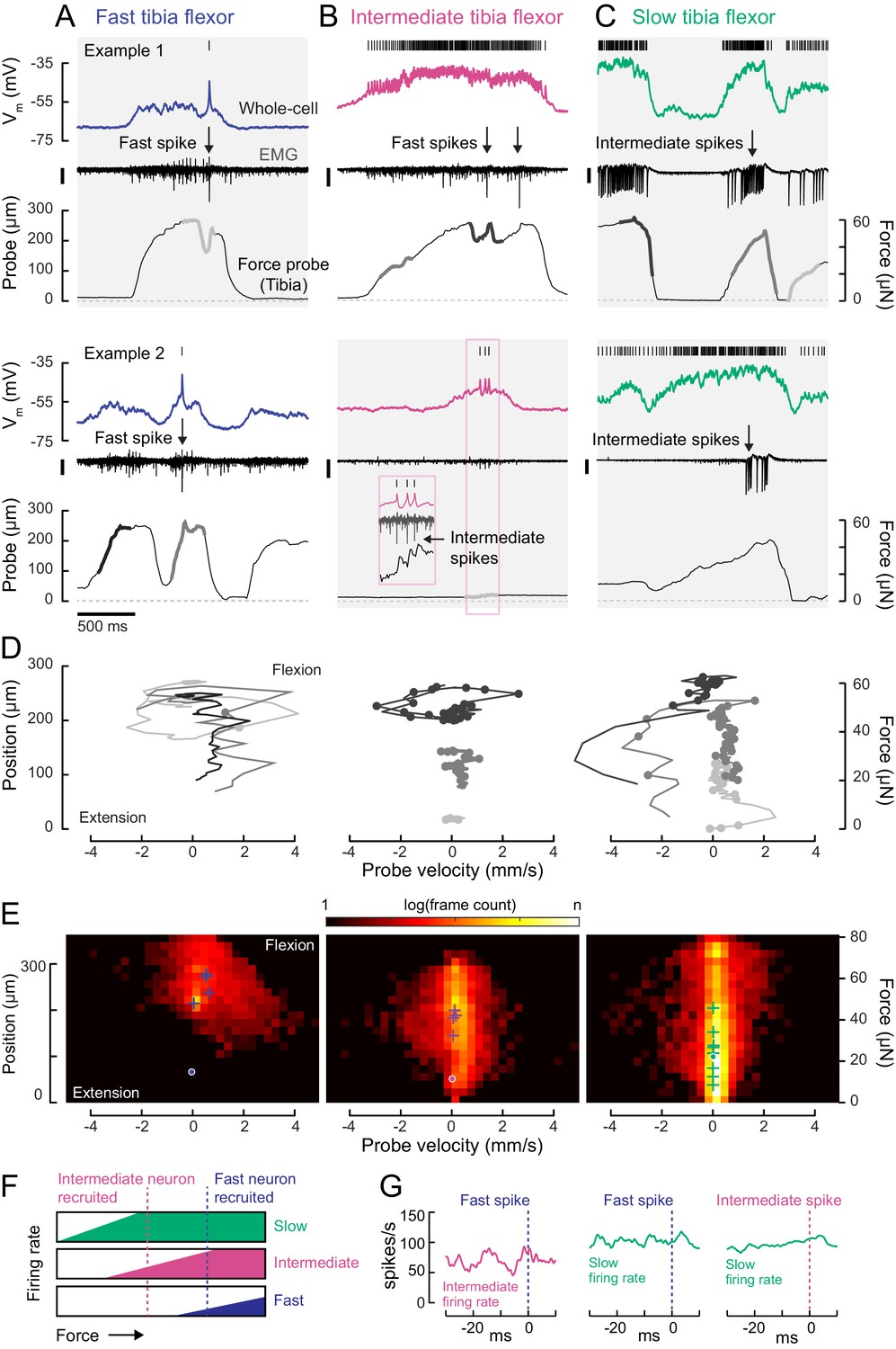
Motor neurons are recruited in a specific order across different motor regimes.
(A) Membrane potential, EMG, and probe movement, for two example epochs of spontaneous leg movement during a whole-cell recording of the fast motor neuron. Highlighted events are plotted in D. The EMG was recorded in the proximal femur to pick up both fast and intermediate spikes (scale is 10 pA). (B) Same as A, but for an intermediate motor neuron. The EMG for the intermediate neuron was recorded in the proximal part of the femur, the largest events reflect activity in the fast motor neuron (scale is 100 pA). (C) Same as A-B, but for a slow motor neuron. The EMG was recorded in the proximal femur, near the terminal bristle, and large events are likely from the intermediate neuron (scale is 100 pA). (D) Example force probe trajectories from movement examples. The grayscale in D matches that of the trajectories in A-C. Each vertex is a single frame; vertices with dots indicate the occurrence of a spike in the whole-cell recording. (E) 2D histograms of probe force and velocity for video frames within 25 ms following a spike across recordings in cells of each type (fast – five neurons, 4666 frames; intermediate – four neurons, 11,833 frames; slow – nine neurons, 65,473 frames). Crosses indicate the centroids of the histograms for individual neurons. Dots outlined in white indicate centroid of the 2D histograms of all frames, within and outside the 25 ms window. Color scale shows the log number of frames in each bin, normalized to the total number of frames. (F) Schematic illustrating firing rate predictions of the recruitment hierarchy. As force increases, left to right, first the slow neuron begins firing, then the intermediate neuron (magenta line). Once the fast neuron spikes, both intermediate and slow neurons are already firing (blue dotted line). (G) Left) Spike rate of intermediate neuron in 30 ms preceding fast EMG spike (n = 4 pairs); center) slow neuron spike rate preceding fast EMG spike (n = 2 pairs); right) and slow neuron spike rate preceding intermediate EMG spike (n = 3 pairs).
Figure 5—figure supplement 1
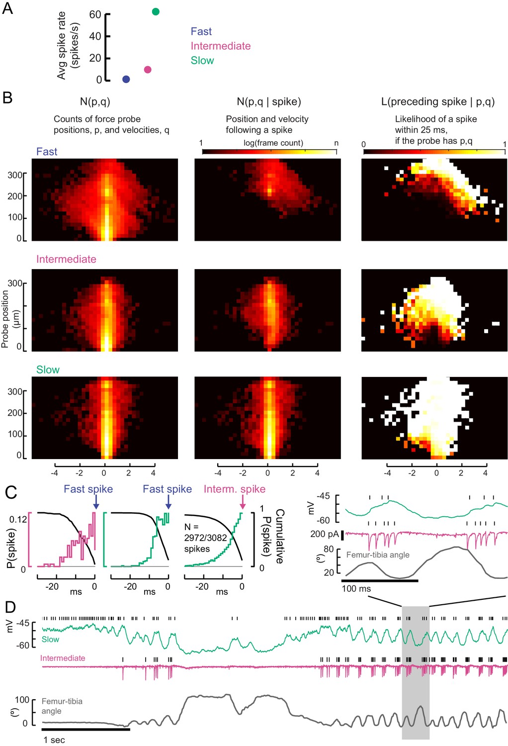
Testing the recruitment hierarchy of motor neurons, in paired recordings and as a function of force probe position and velocity.
(A) The effective spike rate of fast, intermediate and slow motor neurons, over the course of all trials with spontaneous leg movements. Instantaneous spike rates could be much higher. (B) From the 2D spike-triggered phase histograms and Bayes’ rule, we calculated a likelihood function in order to compare spiking regimes in different neurons. If the force probe has a particular position, p, and velocity, q, the likelihood that a motor neuron fired a spike in the preceding 25 ms (right column, linear color scale from 0 to 1) is given by the number of frames with p,q that follow a spike (middle column, shown in Figure 5) divided by the full distribution of p,q (left column). The centroids of the full histograms (left column) are shown in Figure 5. (C) Comparison of activity in recordings of pairs of motor neurons: the number of EMG spikes preceded by a spike in the whole-cell recording, i.e. in a neuron lower down the recruitment hierarchy. The left hand axis indicates the probability of a spike in each millisecond bin for 30 ms before the EMG spike. The right hand axis indicates the cumulative probability of observing a spike in the period before the EMG spike. We found that a small number of intermediate neurons were not preceded by slow neuron spikes (N = 110/3082 spikes). (D) An example trial in which the normal recruitment hierarchy was violated, which only occurred when the leg was unloaded (tibia angle, bottom). During rapid shaking of the leg (highlighted region), the intermediate neuron could spike before the slow motor neuron and have a higher instantaneous spike rate.
Figure 6 with 2 supplements
A gradient of proprioceptive feedback to motor neurons controlling tibia flexion.
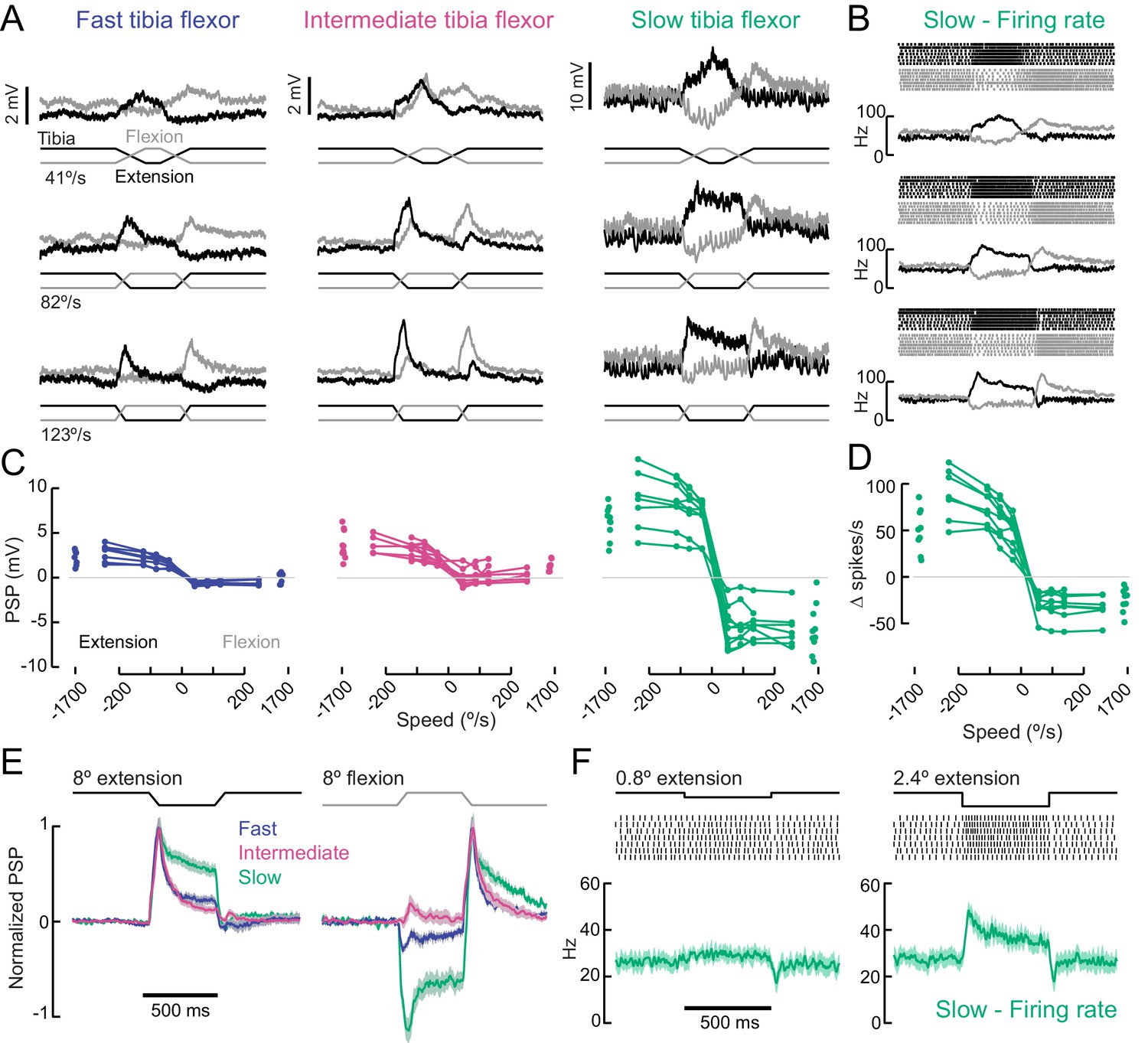
(A) Whole-cell recordings of fast, intermediate, and slow motor neurons in response to flexion (black) and extension (gray) of the tibia. Each trace shows the average membrane potential of a single neuron (n = 7 trials). A 60 μm movement of the probe resulted in an 8° change in femur-tibia angle. (B) Spike rasters and firing rates for the same slow neuron as in A. (C) Amplitude of the postsynaptic potential (PSP) vs. angular velocity of the femur-tibia angle (n = 7 fast, seven intermediate, nine slow cells). Responses to fast extension (−123°/s) are not significantly different for fast and intermediate neurons (p=0.5) but are different for slow neurons (p<10−5, 2-way ANOVA, Tukey-Kramer correction for multiple comparisons). (D) Amplitude of firing rate changes in slow motor neurons vs. angular velocity of the femur-tibia angle. (E) Time-course of normalized average responses (± s.e.m. of baseline subtracted responses) to tibia extension (left) and flexion (right, n = 7 fast, seven intermediate, nine slow cells). (F) Sensitivity of firing rate to small tibia movements of 6 μm (0.8°) or 18 μm (2.4°). Spike rasters are from representative cells, the average spike rate across cells is plotted in green below.
Figure 6—figure supplement 1
Properties of sensory feedback to motor neurons.
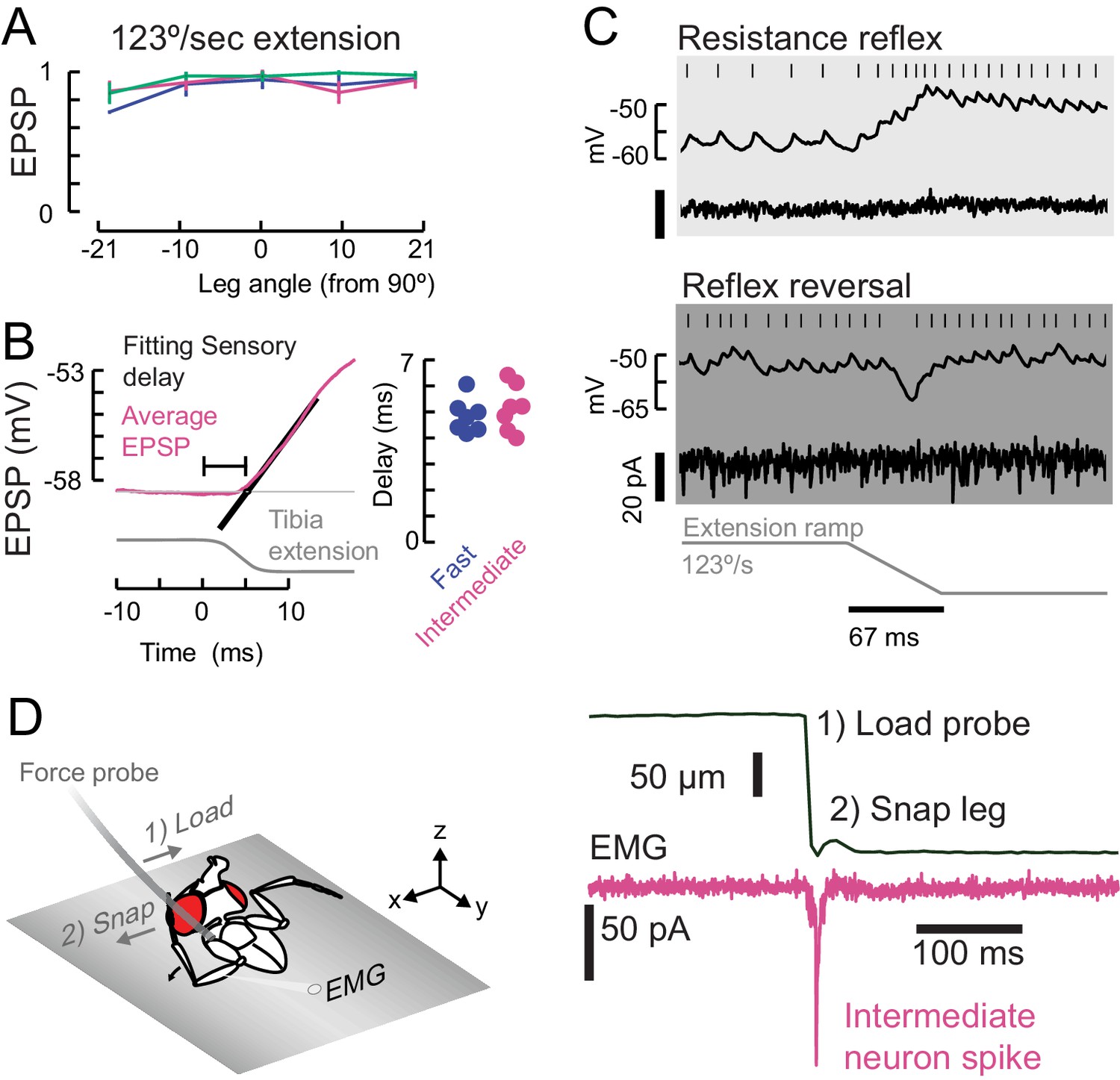
(A) The EPSP evoked by fast ramping extension stimuli did not significantly depend on leg angle. (B) We measured the onset of the sensory evoked EPSP (magenta, intermediate neuron) in the motor neurons by fitting a line (black) to the rising phase of the average response. We measured the time from the start of the command to the piezoelectric actuator for the largest step stimulus (8° extension, shown here as reference). Sensory delays in the fast and intermediate neurons were similar. We did not measure the sensory delays in slow neurons because 1) the spike rate was calculated with an acausal smoothing filter and 2) the average EPSPs were not smooth because of the presence of spikes. (C) An example of reflex reversal in a slow motor neuron. Top) A normal resistance reflex in which an extension of the leg depolarizes the membrane potential and increases the spike rate. Bottom) When the fly was pulling on the force probe and the EMG activity was increased, the extension stimulus instead hyperpolarized the neuron. (D) To test faster stimuli than we could deliver with a piezoelectric actuator, we pulled on the probe with a hook until the hook lost contact, and the probe snapped back to rest. We identified intermediate EMG spikes using optogenetic excitation of R22A08-Gal4 motor neurons. This ballistic stimulus was able to evoke intermediate neuron spikes, but not fast neuron spikes (not shown).
Figure 6—figure supplement 2
Optogenetic activation of proprioceptive sensorimotor circuits.
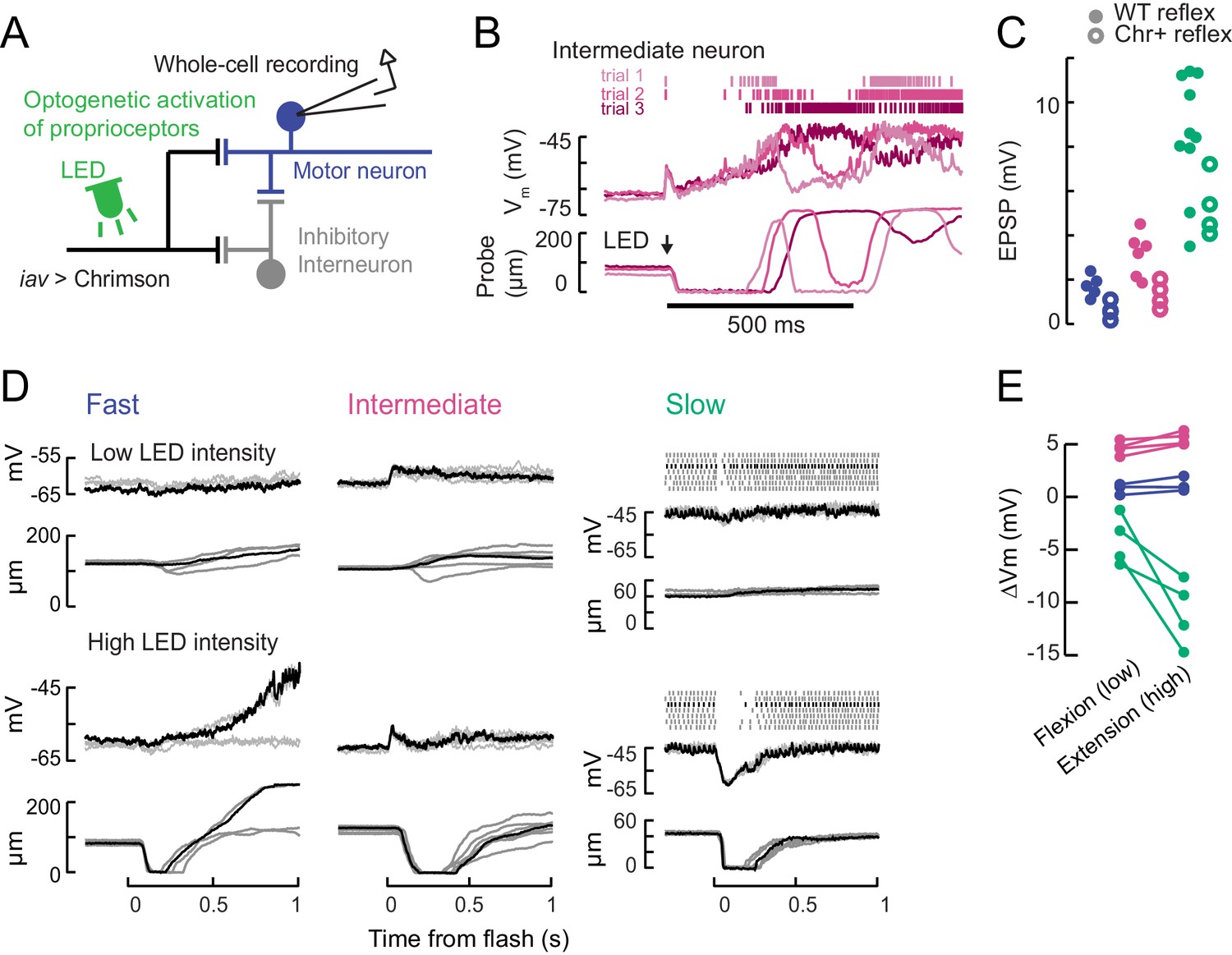
(A) Optogenetic activation of proprioceptive feedback to tibia motor neurons. The axons of femoral chordotonal neurons, labeled by iav-LexA, were stimulated with Chrimson activation during whole-cell recordings. (B) Example responses in an intermediate neuron to a high intensity 10 ms light flash that drove activity in chordotonal neurons expressing Chrimson (iav-LexA >Chrimson). The membrane potential and spikes from three trials are shown above (magenta shading) and the simultaneous force probe movement is shown below. Like the flicking stimulus in Figure 5—figure supplement 1, this large stimulus drove intermediate neurons, but not fast neurons, to spike. The effect of the light stimulus was surprisingly long-lasting, producing membrane potential fluctuations and movements over ~200 ms. (C) Expression of Chrimson decreases gain of proprioceptive feedback. Peak of the average EPSP in fast (blue), intermediate (magenta), and slow (green) motor neurons in response to a ramping extension stimulus (123 °/s), in flies that either express Chrimson in FeCO neurons (Chr+ reflex, empty circles) or not (WT reflex, filled circles). Chrimson expression reduces EPSPs, p<0.01 for all neurons, Wilcoxon rank-sum test. (D) Example recordings showing membrane potential, spiking activity, and probe position following an LED flash. Top: low intensity flashes caused the fly to mainly pull on the force probe, from individual fast (5.5 mW/mm2), intermediate (4.8 mW/mm2), and slow neurons (1.3 mW/mm2). Each trace is a single trial; the black traces belong to the same trial. Bottom: higher LED intensities caused the fly to let go of the force probe in fast (10.9 mW/mm2), intermediate (7.8 mW/mm2), and slow neurons (6.3 mW/mm2). (E) Summary of optogenetically-evoked membrane potential changes in motor neurons for low (flexion-producing) and high (extension-producing) LED intensities. Fast and intermediate neurons depolarized initially, so the amplitude of the depolarization is quantified. Slow motor neurons exhibited stronger hyperpolarization.
Figure 7 with 1 supplement
Optogenetic perturbation of motor neurons in behaving flies.
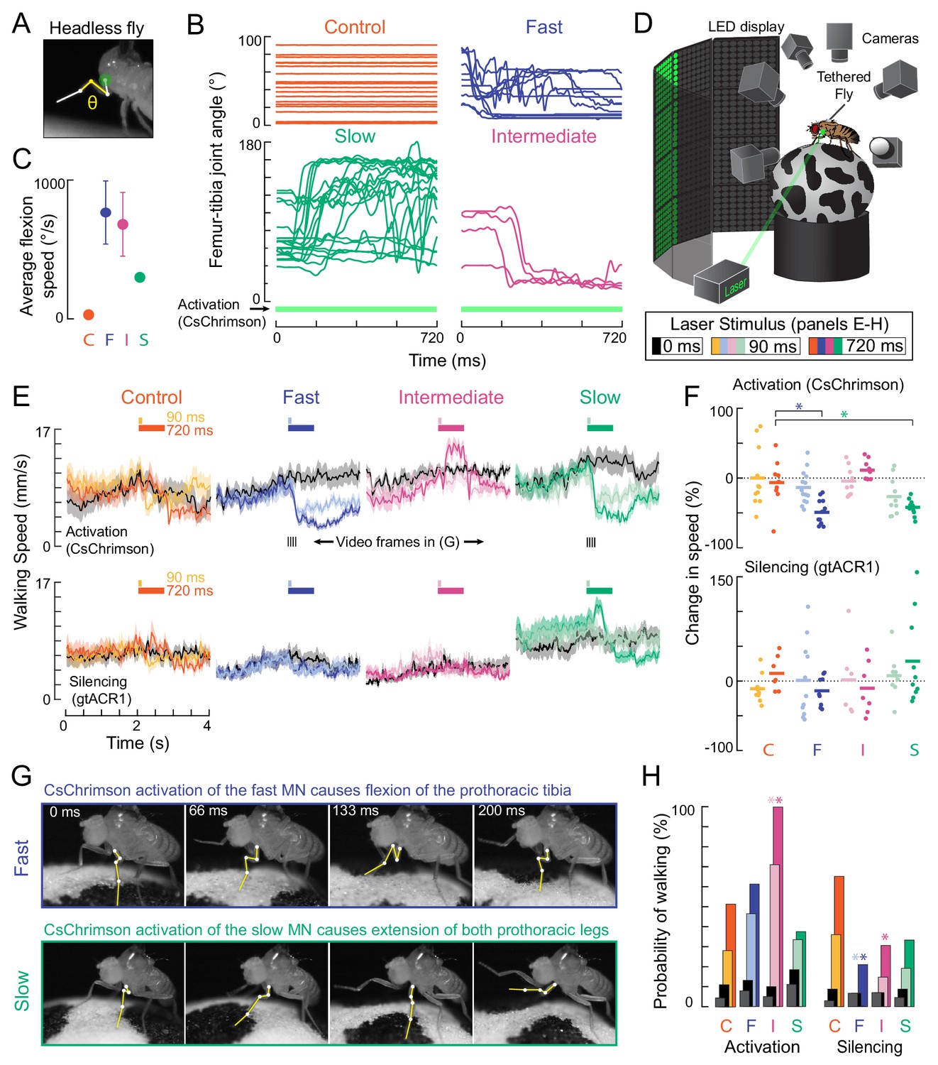
(A) Example frame illustrating behavioral effects of optogenetically activating leg motor neurons in headless flies. A green laser (530 nm) is focused at the coxa-body joint of the fly’s left front leg (outlined in white) and the femur-tibia joint (yellow) is monitored with high-speed video. (B) Example traces of femur-tibia joint angles during optogenetic activation (Gal4 >CsChrimson) of each motor neuron type in headless flies. The control line has the same genetic background as motor neuron lines but lacks Gal4 expression (BDP-Gal4 >CsChrimson).( C) Average (± sem) tibia flexion speed during the first 300 ms of CsChrimson activation (n = 5 flies of each genotype). (D) Schematic of the behavioral setup, in which a tethered fly walks on a spherical treadmill. The treadmill and fly are tracked with separate cameras. As in A), a green laser is focused on the coxa of the left front leg. (E) Average treadmill forward velocity (± sem) of walking flies, when activating (top row) or silencing (bottom row) control (n = 11, 13), fast (n = 15, 14), intermediate (n = 9,12), or slow (n = 11, 13) motor neurons for 90 ms (dark colors) or 720 ms (light colors). Black traces indicate trials with no laser (0 ms). Gray boxes indicate the period of optogenetic stimulation. Black dashes above fast and slow flexor activation traces indicate the time points in panel G. (F) Percent change (change in speed/pre-stimulus speed) in the average running speed of flies shown in C during stimulation+200 ms for activation (top) and silencing (bottom). Asterisks indicate p<0.01 relative to control (bootstrapping with false discovery rate correction; see methods for details). (G) Example frames showing representative behavioral responses of running flies during the first 200 ms of fast (top) and slow (bottom) MN activation. (H) Probability that a stationary fly initiated a walking bout during the 500 ms following either MN activation (left) or silencing (right). Dark colors are for the 90 ms stimulus (or no stimulus – black) and light colors are for the 720 ms stimulus (or no stimulus – gray). Asterisks indicate p<0.01 relative to control (bootstrapping with false discovery rate correction; see Methods for details).
Figure 7—figure supplement 1

Effects of tibia motor neuron silencing and activation on leg kinematics.
(A) Femur-tibia joint angles during silencing (Gal4 >gtACR1) of the three motor neuron types and a control empty Gal4 driver, in headless, suspended flies. (B) Average (± sem) flexion speed during the initial 300 ms of silencing, on trials where the leg moved. (C) Scatter plot of instantaneous flexion speed vs. leg angle for each video frame, when activating (left) or silencing (right) the three motor neuron types (and empty Gal4 control) in headless suspended flies. Extension would be seen as negative and is not shown. The flexion speeds are largest near 80° for trajectories caused by fast neuron activation (blue points).
Videos
Video 1
Calcium imaging of femur muscles.
The video (1) illustrates the arrangement of musculature controlling the fly’s tibia; (2) schematizes the position of a restrained fly relative to the force probe fiber, together with wide-field calcium imaging from muscles in the leg and body; and then (3) shows simultaneous videos of the fly pulling on the force with muscle calcium signals in the femur, together with the movement of the probe, an EMG recording from the fast neuron, and the time course of cluster ΔF/F. Videos are slowed 3X.
Video 2
Motor neuron electrophysiology, force production, and tibia movement.
The video introduces 1) the dendritic morphology and axon projection of the three neurons we studied: fast, intermediate and slow; 2) shows video of individual trials from a fast neuron in which one or four spikes are driven with optogenetic stimulation in the VNC, together with probe movement, the whole-cell current clamp recording from the soma, and the EMG record from the leg; 3) shows video of individual trials from an intermediate neuron in which one or four spikes are driven with optogenetic stimulation in the VNC; 4) shows video of a trial from a slow motor neuron in which current injection at the soma depolarizes the neuron and drives ~ 100 spikes, and a trial in which the slow neuron is hyperpolarized, reducing the force on the probe. Videos are slowed 3X.
Video 3
Optogenetic activation of motor neurons in headless flies.
The video shows the movements of the flies left front tibia caused by optogenetic activation of the fast, intermediate and slow neurons and a control line (BDP-Gal4). The video shows 1) the tibia flexion during the entire 720 ms laser stimulation period slowed 10X; 2) the first 300 ms of the same event, slowed 40X.
Video 4
Optogenetic silencing in all motor neurons controlling the front leg.
Motor neurons labelled by OK371-Gal4 expressed gtACR1. The video shows the behavior of different flies on different trials while 1) flies were walking during a 90 ms laser stimulus; 2) flies were stationary during a 90 ms laser stimulus; 3) flies were walking during a 720 ms laser stimulus; 4) flies were stationary during a 720 ms laser stimulus. Videos of behavior are slowed 10X.
Video 5
Optogenetic activation and silencing of fast motor neurons in behaving flies.
The video shows the behavior of different flies on different trials while 1) flies were walking and the fast neuron expressed CsChrimson; 2) flies were stationary, and the fast neuron expressed CsChrimson; 4) flies were walking, and the fast neuron expressed gtACR1; 3) flies were stationary, and the fast neuron expressed gtACR1. Videos of behavior are slowed 10X.
Video 6
Optogenetic activation and silencing of intermediate motor neurons in behaving flies.
The video shows the behavior of different flies on different trials while 1) flies were walking and the intermediate neuron expressed CsChrimson; 2) flies were stationary, and the intermediate neuron expressed CsChrimson; 3) flies were walking, and the intermediate neuron expressed gtACR1; 4) flies were stationary, and the intermediate neuron expressed gtACR1. Videos of behavior are slowed 10X.
Video 7
Optogenetic activation and silencing of slow motor neurons in behaving flies.
The video shows the behavior of different flies on different trials while 1) flies were walking and the slow neuron expressed CsChrimson; 2) flies were stationary, and the slow neuron expressed CsChrimson; 3) flies were walking, and the slow neuron expressed gtACR1; 4) flies were stationary, and the slow neuron expressed gtACR1. Videos of behavior are slowed 10X.
Video 8
Optogenetic stimulation of a control line (BDP-Gal4).
The video shows the behavior of different control flies on different trials while 1) UAS-CsChrimson flies were walking; 2) UAS-CsChrimson flies were stationary; 3) UAS- gtACR1 flies were walking; 4) UAS- gtACR1 flies were stationary. Videos of behavior are slowed 10X.
Tables
Key resources table
| Reagent type (species) or resource | Designation | Source or reference | Identifiers | Additional information |
|---|---|---|---|---|
| Genetic reagent (D. melanogaster) | ‘w[*]; P{w[+mC]=Mhc-GAL4.K}2’ | Bloomington Drosophila Stock Center | RRID:BDSC_55133 | |
| Genetic reagent (D. melanogaster) | ‘P{y[+t7.7] w[+mC]=20XUAS-IVS-mCD8::GFP}attP2’ | Bloomington Drosophila Stock Center | RRID:BDSC_32194 | |
| Genetic reagent (D. melanogaster) | ‘P{y[+t7.7] w[+mC]=GMR22A08-GAL4}attP2’ | Bloomington Drosophila Stock Center | RRID:BDSC_47902 | |
| Genetic reagent (D. melanogaster) | ‘P{JFRC7-20XUAS-IVS-mCD8::GFP} attp40’ | Other | FBrf0212432 | Barret Pfeiffer, Janelia Farm, HHMI |
| Genetic reagent (D. melanogaster) | ‘MHC-LexA’ | Other | Richard Mann, Columbia University | |
| Genetic reagent (D. melanogaster) | ‘13XLexAop2-IVS-GCaMP6f-p10}su(Hw)attP5’ | Bloomington Drosophila Stock Center | RRID:BDSC_44277 | |
| Genetic reagent (D. melanogaster) | ‘Berlin-K’ | Bloomington Drosophila Stock Center | RRID:BDSC_8522 | |
| Genetic reagent (D. melanogaster) | ‘P{y[+t7.7] w[+mC]=GMR81A07-GAL4}attP2’ | Bloomington Drosophila Stock Center | RRID:BDSC_40100 | |
| Genetic reagent (D. melanogaster) | ‘P{y[+t7.7] w[+mC]=GMR35 C09-GAL4}attP2’ | Bloomington Drosophila Stock Center | RRID:BDSC_49901 | |
| Genetic reagent (D. melanogaster) | ‘10XUAS-syn21-Chrimson88-tDT3.1 (attP18)’ | DOI:10.1016/j.neuron.2017.03.010 | Michael Reiser, Janelia Farm, HHMI | |
| Genetic reagent (D. melanogaster) | ‘P{y[+t7.7] w[+mC]=20 XUAS-IVS-CsChrimson.mVenus}attP2’ | Bloomington Drosophila Stock Center | RRID:BDSC_55136 | |
| Genetic reagent (D. melanogaster) | ‘iav-LexA’ | Bloomington Drosophila Stock Center | RRID:BDSC_52246 | |
| Genetic reagent (D. melanogaster) | ‘13XLexAop2-IVS-Syn-21-Chrimson::tdTomato (attP2)’ | DOI: 10.1038/nmeth.2836 | Barret Pfeiffer, Janelia Farm, HHMI | |
| Genetic reagent (D. melanogaster) | ‘P{y[+t7.7] w[+mC]=BDP-GAL4}attP2’ | DOI:10.7554/eLife.08758.027 | Andrew Seeds, Steffi Hampel, UNIVERSITY OF PUERTO RICO | |
| Genetic reagent (D. melanogaster) | ‘P{w[+mW.hs]=GawB}VGlut[OK371]’ | Bloomington Drosophila Stock Center | RRID:BDSC_26160 | |
| Antibody | nc82 (mouse monoclonal) | Developmental Studies Hybridoma Bank, | RRID:AB_2314866 | 1:50 |
| Chemical compound, drug | MLA | Tocris | TOCRIS_1029 | ‘1 μM methyllycaconitine citrate’ |
| Software, algorithm | MATLAB | Mathworks | RRID:SCR_001622 | |
| Software, algorithm | DeepLabCut | DOI:10.1038/s41593-018-0209-y | Mathis Lab, Rowland Institute, Harvard University https://github.com/AlexEMG/DeepLabCut | |
| Software, algorithm | FIJI | PMID:22743772 | RRID:SCR_002285 | |
| Software, algorithm | Fictrac | DOI:10.1016/j.jneumeth.2014.01.010 | ||
| Other | Force probe fiber | Proform CS2.5 AS | This paper | “PBT fiber from a synthetic paint brush, cut to have a spring constant = 0.22 N/m. Find at any Proform retailer, e.g. Amazon.com’ |
| Other | Green CST DPSS laser, | Besram Technology, Inc | ‘532 nm’ | |
| Other | Phalloidin | ThermoFisherScientific | FISHER: A22284 | ‘633 nm, 1 unit per leg’ |
| Other | streptavidin-Alexa Fluor | ThermoFisherScientific | FISHER: S11226 | ‘568 nm’ |
Additional files
Download links
A two-part list of links to download the article, or parts of the article, in various formats.
Downloads (link to download the article as PDF)
Open citations (links to open the citations from this article in various online reference manager services)
Cite this article (links to download the citations from this article in formats compatible with various reference manager tools)
A size principle for recruitment of Drosophila leg motor neurons
eLife 9:e56754.
https://doi.org/10.7554/eLife.56754


