The roles of online and offline replay in planning
Figures
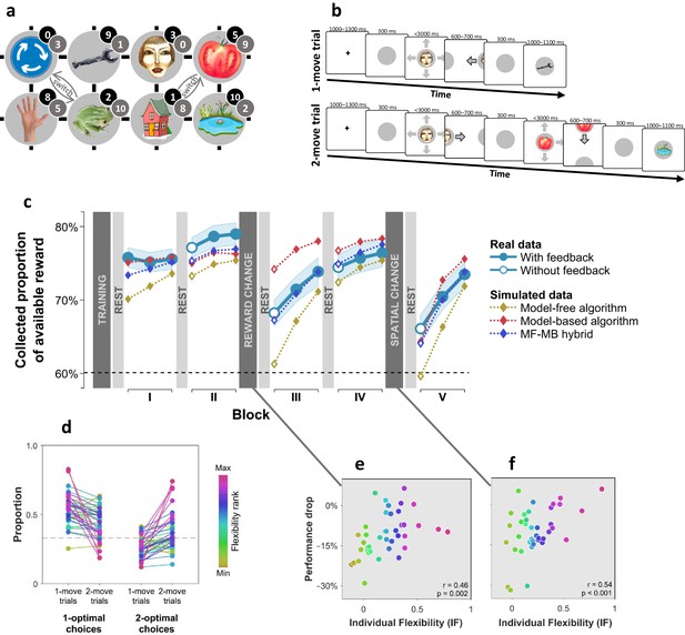
Subjects differed in decision flexibility.
(a) Experimental task space. Before performing the main task, subjects learned state-reward associations (numbers in black circles) and they were then gradually introduced to the state space in a training session. After performing the main task for two blocks of trials, subjects learned new state-reward associations (numbers in dark grey circles) and then returned to the main task. Before a final block of trials, subjects were informed of a structural task change such that ‘House’ switched position with ‘Tomato’, and ‘Traffic sign’ switched position with ‘Frog’. The bird’s eye view shown in the figure was never seen by subjects. Subjects only saw where they started from on each trial and, after completing a move, the state to which their move led. The map was connected as a torus (e.g., starting from ‘Tomato’, moving right led to ‘Traffic sign’, and moving up or down from the tomato led to ‘Pond’). (b) Each trial started from a pseudorandom location from whence subjects were allowed either one (‘1-move trial’) or two (‘2-move trial’) consecutive moves (signalled at the start of each set of six trials), before continuing to the next trial. Outcomes were presented as images alone, and the associated reward points were not shown. A key design feature of the map was that in 5 out of 6 trials the optimal (first) move was different depending on whether the trial allowed for one or two moves. For instance, given the initial image-reward associations (black) and image positions, the best single move from ‘Face’ is LEFT (9 points), but when two moves are allowed the best moves are RIGHT and then DOWN (5+9 giving 15 total points). Note that the optimal moves differed also given the second set of image-reward associations. On ‘no-feedback’ trials (which started all but the first block), outcome images were also not shown (i.e., in the depicted trials, the ‘Wrench’, ‘Tomato’ and ‘Pond’ would appear as empty circles). (c) The proportion of obtainable reward points collected by the experimental subjects, and by three simulated learning algorithms. Each data point corresponds to 18 trials (six 1-move and twelve 2-move trials), with 54 trials per block. The images to which subjects moved were not shown to subjects for the first 12 trials of Blocks II to V (the corresponding ‘Without feedback’ data points also include data from 6 initial trials with feedback wherein starting locations had not yet repeated, and thus, subjects’ choices still reflected little new information). All algorithms were allowed to forget information so as to account for post-change performance drops as best fitted subjects’ choices (see Materials and methods for details). Black dashed line: chance performance. Shaded area: SEM. (d) Proportion of first choices that would have allowed collecting maximal reward where one (‘1-optimal’) or two (‘2-optimal’) consecutive moves were allowed. Choices are shown separately for what were in actuality 1-move and 2-move trials. Subjects are colour coded from lowest (gold) to highest (red) degree of flexibility in adjusting to one vs. two moves (see text). Dashed line: chance performance (33%, since up and down choices always lead to the same outcome). (e,f) Decrease in collected reward following a reward-contingency (e) and spatial (f) change, as a function of the index of flexibility (IF) computed from panel d. Measures are corrected for the impact of pre-change performance level using linear regression. value derived using a premutation test.
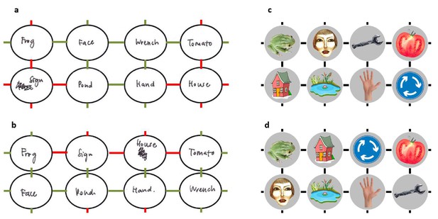
Example sketches of the state space by a representative subject.
Subjects sketched the state space at the end of the experiment, recalling how it had been structured before (a) and after (b) the position change. On average, subjects sketched much of the state spaces accurately (correct state transitions: first map , ; second map , ; chance = 0.14, , Bootstrap test). (a,b) Sketches by a representative subject with 0.58 accuracy for the state space before (a) and after (b) the spatial change. Erroneous transitions are marked in red. (c,d) The actual state spaces the subject navigated before (c) and after (d) the position change.
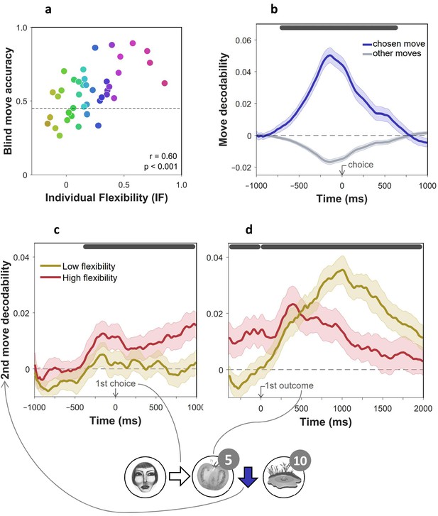
Evidence of advance prospective planning in flexible subjects.
= 40 subjects. (a) Proportion of optimal choices in second moves for trials without feedback, as a function of individual index of flexibility (IF). In such trials, second moves were enacted without seeing the state they were made from. Measures are corrected using linear regression for accuracy of non-blind moves from the same phases of the experiment. (b) Validation of move decoder. The plot shows the decodability of chosen and unchosen moves from MEG data recorded during the main task. Decodability was computed as the probability assigned to the chosen move (right, left, up or down) by a 4-way classifier based on each timepoint’s spatial MEG pattern, minus the average probability assigned to the same moves at baseline (400 ms preceding trial onset). A separate decoder was trained for each subject on MEG data recorded outside of the main task, during the image-reward association training phases. (c,d) Decodability of second moves (the blue arrow in the bottom example cartoon) in 2-move trials during first move choice (c) and presentation of the first outcome (d), as a function of IF. For display purposes only, mean time series are shown separately for subjects with high (above median) and low (below median) IF. In all panels, dark gray bars indicate timepoints where the 95% Credible Interval excludes zero and Cohen’s d > 0.1 (Bayesian Gaussian Process analysis). Dashed lines: chance decodability level.
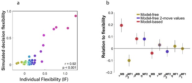
Individual flexibility reflected the balance between MB and MF planning.
= 40 subjects. (a) Actual and simulated individual flexibility (IF). Task performance was simulated using subjects’ best-fitting parameter settings. IF was computed for each simulated subject and averaged over 100 simulations. (b) Relationship between IF and individually-fitted parameters. IF was regressed on subjects’ best-fitting parameter settings, including all learning (), memory (), and inverse temperature () parameters. Parameters are color-coded by the component of the algorithm they enhance. Error bars: 95% CI.
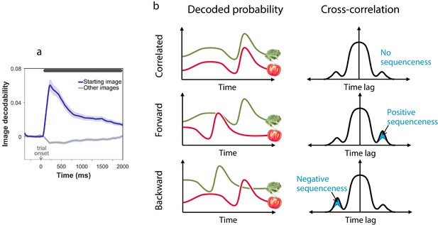
Sequenceness analysis.
(a) Validation of the image MEG decoder used for the sequenceness analyses. = 40 subjects. The plot shows the decodability of starting images from MEG data recorded during the main task at trial onset. Decodability was computed as the probability assigned to the starting image by an 8-way classifier based on each timepoint’s spatial MEG pattern, minus chance probability (0.125). (b) Schematic depiction of the sequenceness analysis used to determine whether representational probabilities of pairs of elements followed one another in time. Sequenceness is computed as the difference between the cross-correlation of two time series with positive and negative time lags. Since it focuses on asymmetries in the cross correlation function, this measure is useful for detecting sequential relationships even between closely correlated (or anti-correlated) time series. Negative sequenceness indicates signals are ordered in reverse.
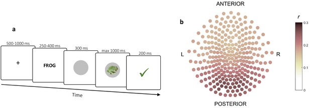
Decoding procedure.
(a) Pre-task stimulus exposure on which decoders were trained. Timeline of a trial. (b) Decoding contribution by sensor. Contribution was quantified as the Spearman correlation between MEG signal and decoder output within trials for each stimulus. Correlations were then averaged over stimuli, trials and subjects.
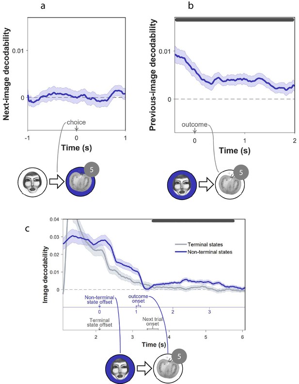
Previous, not subsequent, states were encoded in MEG.
(a) Decodability during choice, of the image to which the chosen move led subsequently. (b) Decodability following outcome, of images subjects had visited earlier in the trial. In panels a and b, the analysis excluded decoded probabilities assigned to the image presently on the screen. Dark gray bars indicate timepoints where the 95% Credible Interval excludes zero and Cohen’s (Bayesian Gaussian Process analysis). Dashed lines: chance decodability level. Example trials are shown below the plots with decoded elements marked in blue. (c) Decoding is shown separately for non-terminal states from which subjects moved (here face) and for trials’ terminal states, while aligning the offsets of both types of state. The top (blue) and bottom (grey) x axes denote time of non-terminal and terminal state decoding, respectively, given that the terminal state is the outcome of the non-terminal state. Non-terminal states were followed by outcomes (here tomato) within 1 to 1.1 s. By comparison, terminal states were followed by a new trial within 1.3 to 1.6 s. The top bar indicates significant post-outcome decodability (p < 0.001, permutation test). Examination of the entire sample (n = 40) shows post-outcome decodability was higher in subjects with greater evidence of on-task sequenceness (r = 0.32, p = 0.04, permutation test).
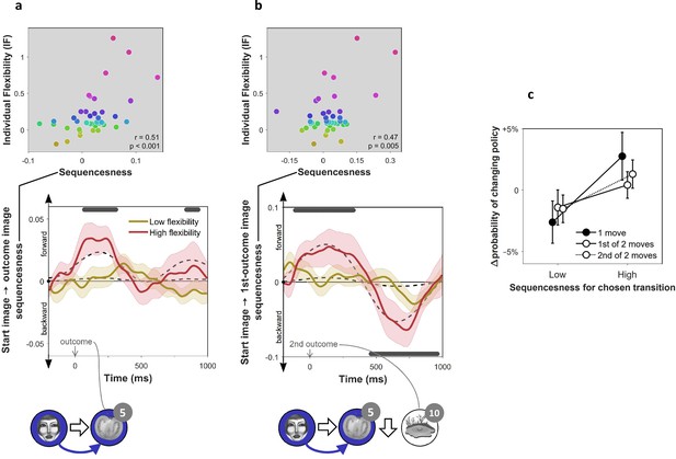
On-task replay of state-to-state trajectories as a function of individual flexibility.
= 40 subjects. (a) Sequenceness corresponding to a transition from the image the subject had just left (‘Start image’; in the cartoon at the bottom, the face) to the image to which they arrived (‘outcome image’; the tomato) following highly surprising outcomes (i.e., above-mean state prediction error). In the cartoon, the white arrow indicates the actual action taken on the trial; the blue arrow indicates the sequence that is being decoded. For display purposes alone, mean time series are shown separately for subjects with high (above median) and low (below median) IF. Positive sequenceness values indicate forward replay and negative values indicate backward replay. As in previous work (Eldar et al., 2018), sequenceness was averaged over all inter-image time lags from 10 ms to 200 ms, and each timepoint reflects a moving time window of 600 ms centred at the given time (e.g., the 1 s timepoint reflects MEG data from 0.7 s to 1.3 s following outcome). Dashed lines show mean data generated by a Bayesian Gaussian Process analysis, and the dark gray bars indicate timepoints where the 95% Credible Interval excludes zero and Cohen’s d > 0.1. The top plot shows IF as a function of sequenceness for the timepoint where the average over all subjects was maximal. value derived using a premutation test. Dot colours denote flexibility rank. (b) Sequenceness following the conclusion of 2-move trials corresponding to a transition from the starting image to the first outcome image. (c) Difference in the probability of subsequently choosing a different transition as a function of sequenceness recorded at the transition’s conclusion. For display purposes only, sequenceness is divided into high (i.e., above mean) and low (i.e., below mean). A correlation analysis between sequenceness and probability of policy change showed a similar relationship (Spearman correlation: , , , Bootstrap test). Sequenceness was averaged over the first cluster of significant timepoints from panels b) and c), in subjects with non-negligible inferred sequenceness (more than the standard deviation divided by 10; ), for the first time the subject chose each trajectory. Probability of changing policy was computed as the frequency of choosing a different move when occupying precisely the same state again. 0 corresponds to the average probability of change (51%). Error bars: s.e.m.
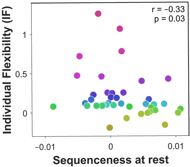
Off-task replay of past and future trajectories.
= 40 subjects. Individual flexibility as a function of sequenceness in rest MEG data for the five most frequently experienced image-to-image transitions. For each rest period, sequenceness was averaged over transitions from both the preceding and following blocks of trials. value derived using a premutation test. Dot colours denote flexibility rank.
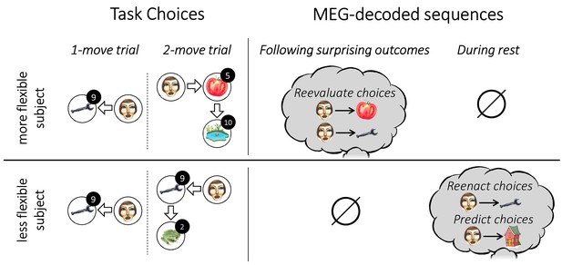
Individual flexibility and evidence of replay.
The figure illustrates typical results for individuals with low (i.e., below median) and high (i.e., above median) flexibility. More flexible subjects advantageously adjusted their choices to the number of allotted moves. Such flexibility was associated with evidence of primarily forward replay following surprising outcomes, encoding the chosen transitions that led to those outcomes, and coupled with a reevaluation of those choices. Less flexible subjects showed evidence of forward replay during rest, encoding previously and subsequently chosen transitions.


