Figures and data in A flexible framework for simulating and fitting generalized drift-diffusion models

Figures
Tables
Additional files

5 figures, 2 tables and 1 additional file

Figures

Figure 1

Download asset Open asset

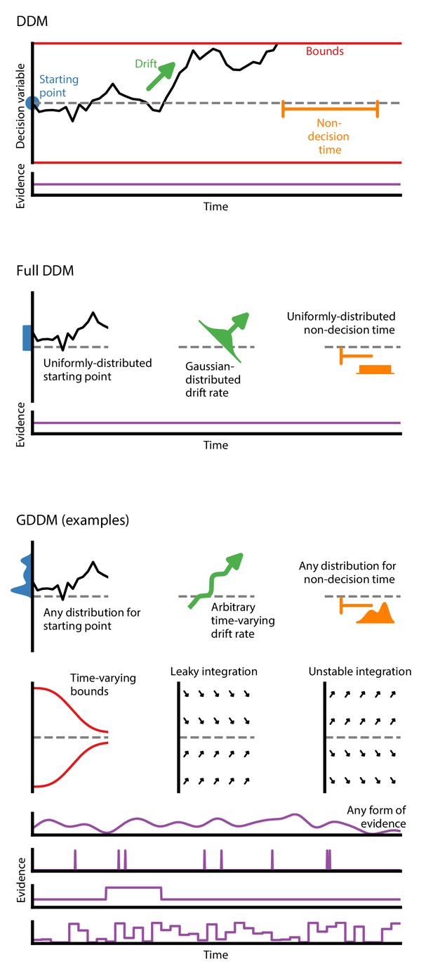
Generalized DDM.

The DDM has fixed, limited parameters, and requires a stream of constant evidence. The ‘full DDM’ expands on the DDM by allowing uniformly-distributed starting position or non-decision time and Gaussian-distributed drift rate. The GDDM is a generalization of the DDM framework which allows arbitrary distributions for starting position and non-decision time, as well as arbitrary functions (instead of distributions) for drift rate and collapsing bounds. It also permits experimental paradigms with dynamic evidence. Several examples of potential GDDM mechanisms are shown. In each case, total response time is the time to reach the diffusion bound plus the non-decision time.

Figure 2 with 3 supplements

Download asset Open asset

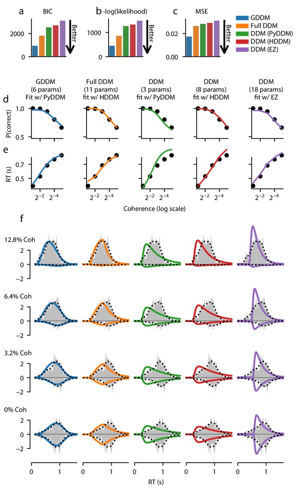
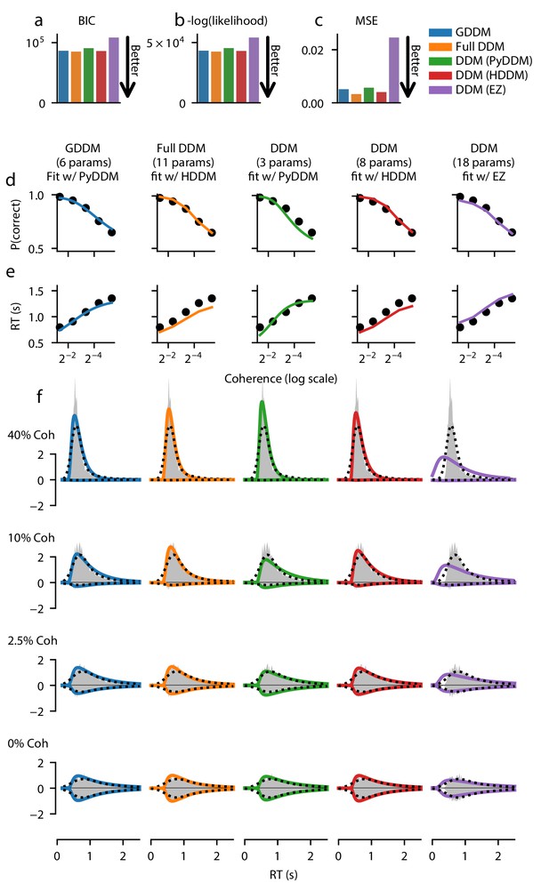
Fit of DDM, ‘full DDM’, and GDDM to Roitman and Shadlen, 2002.

Five models (see **Materials and methods**) were fit with three different software packages to data from monkey N. Model fits are compared according to BIC (a), negative log likelihood (b), and mean squared error (MSE) (c). The psychometric (d) and chronometric (e) functions represent data as dots and models as lines. The probability density function (PDF) (f) of each model is shown for 12.8% coherence, 6.4% coherence, 3.2% coherence, and 0% coherence. The data RT histogram is shown in gray, and black dots show the smoothed kernel density estimate probability distribution derived from the data (Scott, 2015). Columns of the figure and the color of the line denote different models.

Figure 2—figure supplement 1

Download asset Open asset

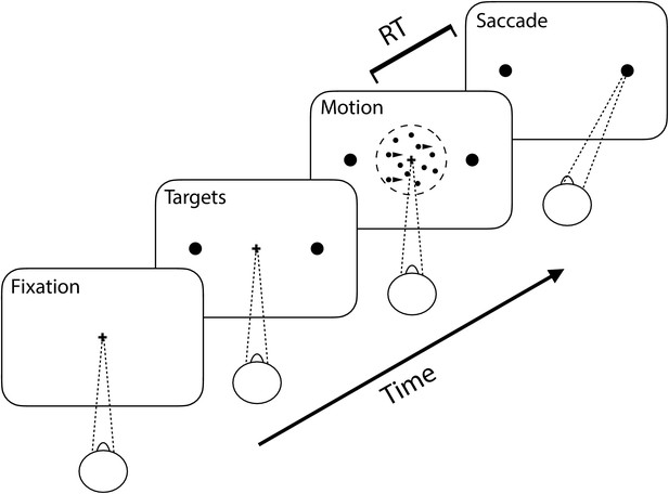
Random dot motion task.

Two rhesus monkeys performed a perceptual decision-making task. Visual stimuli consisted of randomly placed dots on a screen which each moved independently to the left or right. The monkey was required to determine the majority direction of the dots. Task difficulty was varied by changing the fraction of dots which moved coherently in a single direction.

Figure 2—figure supplement 2

Download asset Open asset

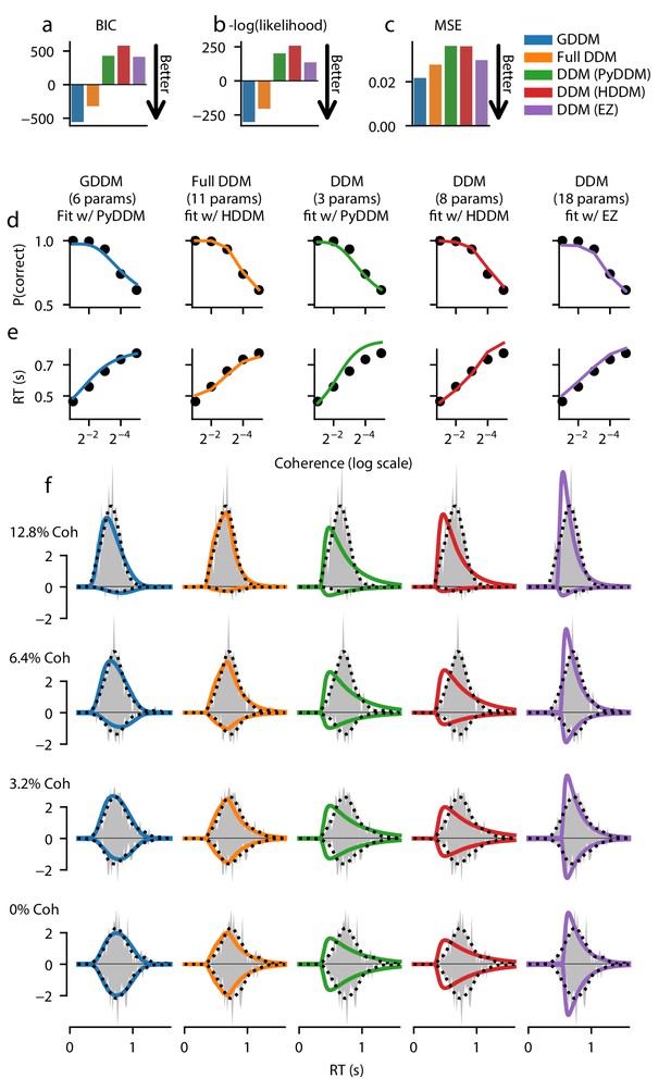
Fit of DDM and GDDM in monkey B.

Format similar to Figure 2.

Figure 2—figure supplement 3

Download asset Open asset

Fit of DDM and GDDM to Evans and Hawkins, 2019.

Format similar to Figure 2. For this dataset, from human subjects, this GDDM did not improve the fit compared to the DDM or ‘full DDM’.

Figure 3

Download asset Open asset

Methods for estimating GDDM RT distributions.

(a) A schematic of trial-wise trajectory simulation methods. In a single trial, a subject’s decision process can be summarized by a stochastic decision variable (DV); simulating this single-trial decision variable many times results in a histogram approximation to the RT distribution. (b) A schematic of solving the Fokker-Planck equation. The full probability distribution of decision variables is solved at each time point, providing a numerical solutions with higher accuracy and reduced execution time.

Figure 4 with 2 supplements

Download asset Open asset

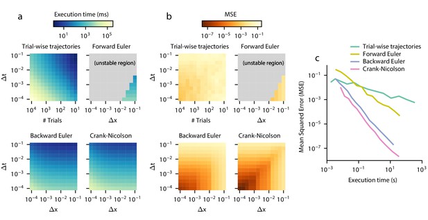
Execution time vs error tradeoff.

A DDM with constant drift, noise, and bounds was estimated for different spatial (Δx) and temporal (Δt) resolutions. Execution time (a) and MSE (b) are shown across values of Δx and Δt. MSE was computed against the analytical DDM solution for the full distribution. Darker colors indicate a more favorable execution time vs error tradeoff. Gray color indicates numerical instability. (c) Relationships between execution time and error which approximately maximize this tradeoff are shown. Parametric expressions were empirically determined to approximately maximize accuracy vs error tradeoff (see Figure 4—figure supplement 1), and are given by $Δ t = 0.43 Δ x^{2}$ for forward Euler and $Δ t = Δ x$ for trial-wise trajectory simulation, backward Euler, and Crank-Nicolson. The lower left indicates low error and fast execution time whereas the upper right indicates slow execution time and high error.

Figure 4—figure supplement 1

Download asset Open asset

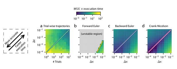
Execution time vs MSE tradeoff across parameters.

As a proxy for the execution time vs error tradeoff, mean squared error (MSE) multiplied by execution time in seconds is shown for several values of Δx and Δt for each method. The lower left corner is the most accurate, and the upper right corner is the fastest. Darker colors indicate more favorable values.

Figure 4—figure supplement 2

Download asset Open asset

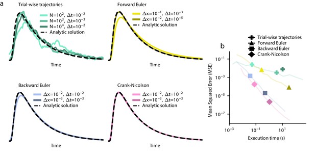
Example estimated RT distributions with different numerical parameters.

(a) Example traces are shown for all four methods. These traces are compared to the analytic solution, shown as a dotted black line. (b) The execution time is plotted against the accuracy. Lines from Figure 4c are plotted in light colors for comparison. Note that not all points fall on these lines because the points don’t necessarily satisfy the constraints on Δx and Δt from Figure 4c and Figure 4—figure supplement 1.

Figure 5 with 2 supplements

Download asset Open asset

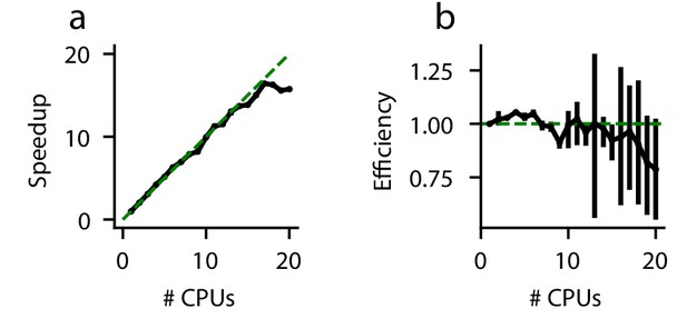
Parallel performance.

Simulations of a standard DDM were performed, varying numbers of CPUs each with ten replicates. (a) The speedup, defined as (execution time on 1 CPU)/(execution time on N CPUs), and (b) parallel efficiency, defined as speedup/(N CPUs), are shown for different numbers of CPUs. Because measured execution time varied run to run, the mean parallel efficiency could sometimes exceed 1. Error bars are bootstrapped 95% confidence intervals. Solid black lines indicate data, and dashed green lines indicate the theoretical maximum under noiseless conditions. Confidence intervals in (a) are hidden beneath the markers.

Figure 5—figure supplement 1

Download asset Open asset

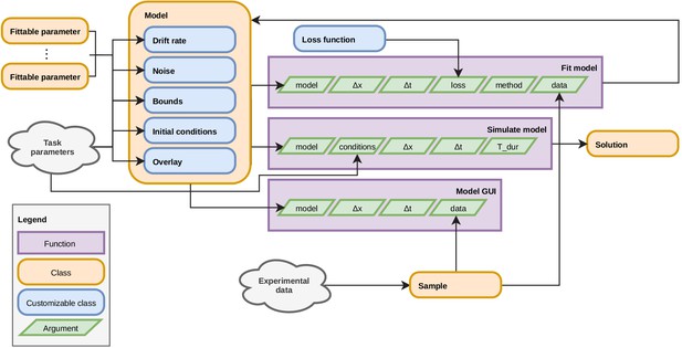
Organization of PyDDM’s source code.

The PyDDM source code is organized in a way which mirrors the GDDM framework. Each model is built by defining five components, analogous to those described in ‘GDDM description’. Each of these components may have any number of fittable parameters, and these parameters may be shared across model components. They may also depend on task parameters, which vary trial to trial. There are three central functions which may be performed on a model: it may be fit to data, it can be simulated for a specific trial type (i.e. with a given set of task parameters), or it may visualized using the GUI.

Figure 5—figure supplement 2

Download asset Open asset

Model GUI.

The PyDDM GUI allows the user to interactively change the parameters of their model (right pane) and see how these changes are reflected in the RT distribution. This makes it possible to gain an intuition for how various parameters and interactions among parameters impact the shape of the RT distribution. The GUI may be used with or without experimental data. When experimental data are provided the model’s simulated RT distribution is overlaid on the empirical RT histogram. The data may be shown all at once, or subset by experimental condition (left pane). Shown here are the data from Roitman and Shadlen, 2002 and the 5-parameter GDDM from Figure 2.

Tables

Table 1

Methods for estimating RT distributions, in order of priority within PyDDM.

	Time accuracy	Grid accuracy	Requirements
Analytical	Exact	Exact	Time- and position-independent drift rate, diffusion constant, and bounds (or linearly collapsing bounds); centered point source initial condition
Crank-Nicolson	$O (Δ t^{2})$	$O (Δ x^{2})$	Time independent bounds
Backward Euler	$O (Δ t)$	$O (Δ x^{2})$	None (fallback for all models)

Forward Euler	$O (Δ t)$	$O (Δ x^{2})$	Numerics $Δ t / Δ x^{2} < 1 / σ^{2}$ (not used by PyDDM)
Trial-wise trajectories	N/A	N/A	(not used by PyDDM)

Table 2

Comparison of existing DDM packages.

PyDDM is compared to HDDM (Wiecki et al., 2013), EZ-Diffusion (Wagenmakers et al., 2007), CHaRTr (Chandrasekaran and Hawkins, 2019), Diffusion Model Analysis Toolbox (DMAT) (Grasman et al., 2009; Vandekerckhove and Tuerlinckx, 2008), and fast-dm (Voss and Voss, 2007; Voss and Voss, 2008; Voss et al., 2015). Red indicates limited flexibility, yellow indicates moderate flexibility, and green indicates maximal flexibility. For the solver, these colors indicate minimal, moderate, and maximal efficiency.

	PyDDM	HDDM	EZ-Diffusion	CHaRTr	DMAT	fast-dm
Language	Python3	Python2/3	Matlab, R, Javascript, or Excel	Requires both R and C	Matlab	Command line
Solver	Fokker-Planck, analytical	Analytical numerical hybrid	None	None (Monte Carlo)	Analytical numerical hybrid	Fokker-Planck
Task parameters
Time dependence of drift/noise	Any function	Constant	Constant	Any function	Constant	Constant
Position dependence of drift/noise	Any function	Constant	Constant	Any function	Constant	Constant
Bounds	Any function	Constant	Constant	Any function	Constant	Constant
Parameter dependence on task conditions	Any relationship for any parameter	Regression model	Categorical	Categorical	Linear	Categorical
Across-trial variability
Across-trial drift variability	Slow discretization (via extension)	Normal distribution	None	Any distribution	Normal distribution	Normal distribution
Across-trial starting point variability	Any distribution	Uniform distribution	None	Any distribution	Uniform distribution	Uniform distribution
Across-trial non-decision variability	Any distribution	Uniform distribution	None	Any distribution	Uniform distribution	Uniform distribution
Model simulation and fitting
Hierarchical fitting	No	Yes	No	No	No	No
Fitting methods	Any numerical (default: differential evolution)	MCMC	Analytical	Any numerical	Nelder-Mead	Nelder-Mead
Objective function	Any function (default: likelihood)	Likelihood	Mean/stdev RT and P(correct)	Any sampled (e.g. quantile maximum likelihood)	Quantile maximum likelihood or chi-squared	Likelihood, chi-squared, Kolmogorov-Smirnov
Mixture model	Any distribution(s)	Uniform	None (extendable)	None	Uniform and undecided guesses	Uniform