Uncovering the computational mechanisms underlying many-alternative choice
- Technische Universität Berlin, Germany
- Freie Universität Berlin, Germany
- Center for Cognitive Neuroscience Berlin, Germany
- Max Planck School of Cognition, Germany
- WZB Berlin Social Science Center, Germany
- The Ohio State University, United States
Figures
Figure 1 with 3 supplements
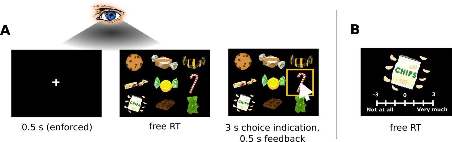
Choice task.
(A) Subjects chose a snack food item (e.g., chocolate bars, chips, gummy bears) from choice sets with 9, 16, 25, or 36 items. There were no time restrictions during the choice phase. Subjects indicated when they had made a choice by pressing the spacebar of a keyboard in front of them. Subsequently, subjects had 3 s to indicate their choice by clicking on their chosen item with a mouse cursor that appeared at the centre of the screen. Subjects used the same hand to press the space bar and navigate the mouse cursor. For an overview of the choice indication times (defined as the time difference between the spacebar press and the click on an item), see Figure 1—figure supplement 3. Trials from the four set sizes were randomly intermixed. Before the beginning of each choice trial, subjects had to fixate a central fixation cross for 0.5 s. Eye movement data were only collected during the central fixation and choice phase. (B) After completing the choice task, subjects indicated how much they would like to eat each snack food item on a 7-point rating scale from −3 (not at all) to 3 (very much). For an overview of the liking rating distributions, see Figure 1—figure supplements 1, 2. The tasks used real food items that were familiar to the subjects.
Figure 1—figure supplement 1

Liking rating distribution of each subject.
Figure 1—figure supplement 2
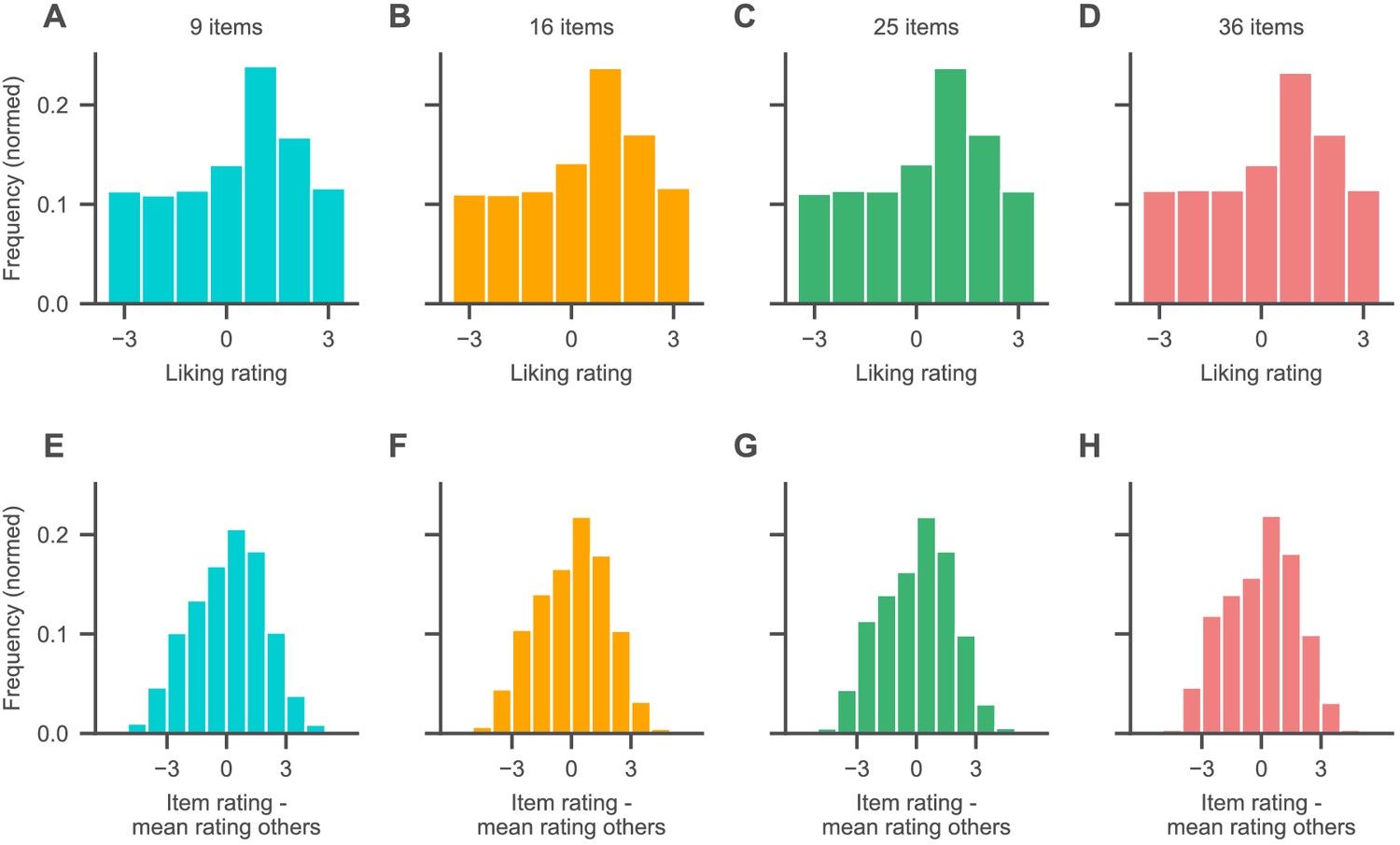
Absolute (A–D) and relative (E–H; defined as the difference between an item’s rating and the mean rating of the other items in a choice set) liking rating distributions for each set size.
Figure 1—figure supplement 3
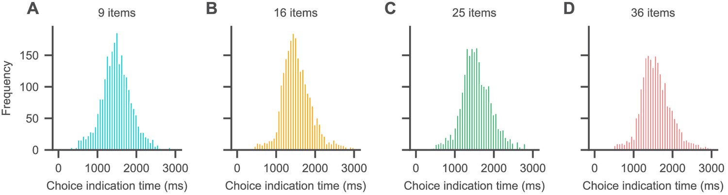
Choice indication times for each set size as indicated by the time difference between space bar press (indicating RT) and subsequent mouse click on a snack food item image.
For details on the experiment paradigm, see the Materials and methods section of the main text. Choice indication times generally increased with the Euclidean distance of the chosen item from the screen centre (where the mouse cursor appeared) as well as set size (intercept = 1256 ms, 94% highest density intervals (HDI) = [1178, 1337], = 0.59 ms, 94% HDI = [0.52, 0.66] per pixel increase in Euclidean distance, 2.3 ms, 94% HDI = [1.6, 3] per item). Note that the intercept estimate of 1256 ms describes the average time that it took subjects to move their hand from the space bar to the computer mouse and added time resulting from movement noise in the mouse trajectory.
Figure 2
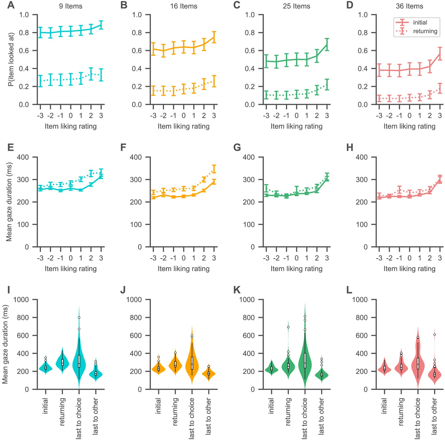
Gaze psychometrics for each set size.
(A–H) The probability of looking at an item (A–D) as well as the mean duration of item gazes (E–H) increases with the liking rating of the item. Solid lines indicate initial gazes to an item, while dotted lines indicate all subsequent returning gazes to the item. (I–L) Initial gazes to an item are in general shorter in duration than all subsequent gazes to the same item in a trial. The last gaze of a trial is in general longer in duration if it is to the chosen item than when it is to any other item. See the Visual search section for the corresponding statistical analyses. Colours indicate set sizes. Violin plots show a kernel density estimate of the distribution of subject means with boxplots inside of them.
Figure 3
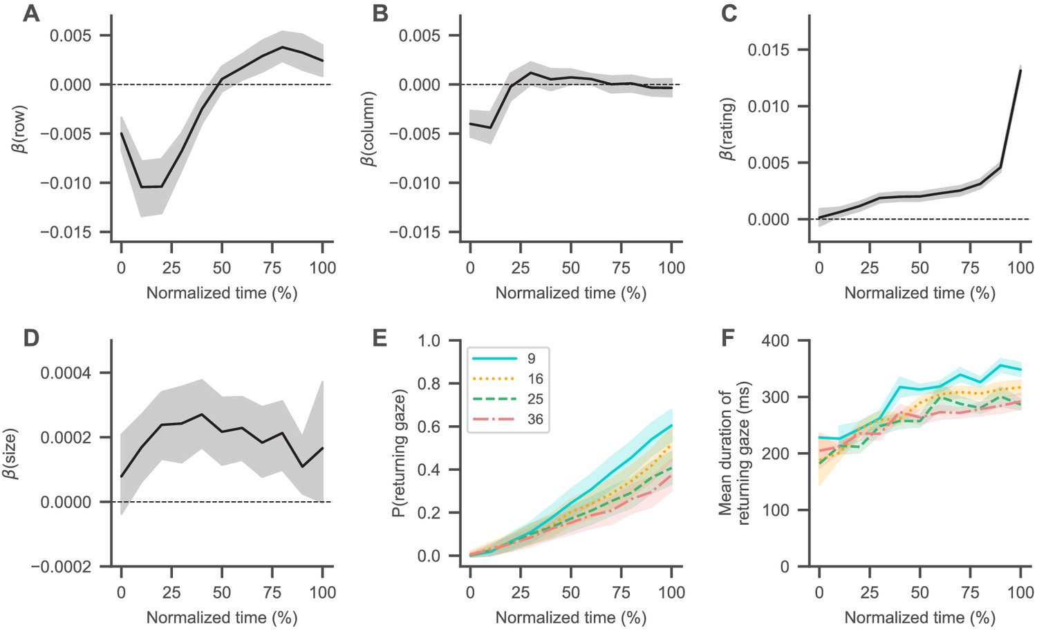
Visual search trajectory.
(A–D) Black lines represent the fixed-effects coefficient estimates (with 94% HDI intervals surrounding them) of a mixed-effects logistic regression analysis (see Materials and methods) for each normalized trial time bin regressing the probability that an item was looked at onto its centred attributes (row (A) and column (B) position, liking rating (C), and size (D); see Materials and methods). Subjects generally started their search in the centre of the choice screen, coinciding with the fixation cross, and then transitioned to the top left corner (as indicated by decreasing regression coefficients for the items’ row (A) and column positions (B)). From there, subjects generally searched from top to bottom (as indicated by slowly increasing regression coefficients for the items’ row positions (A)), while also focusing more on items with a high liking rating (C) and a larger size (D). Dashed horizontal lines indicate a coefficient estimate of 0. (E, F) Over the course over a trial, subjects were more likely to look at items that they had already seen in the trial (E), while the duration of these returning gazes also increased (F). See the Visual search section for details on the corresponding statistical analyses. Coloured lines in (E) and (F) indicate mean values with standard errors surrounding them, while colours and line styles represent set size conditions.
Figure 4 with 2 supplements
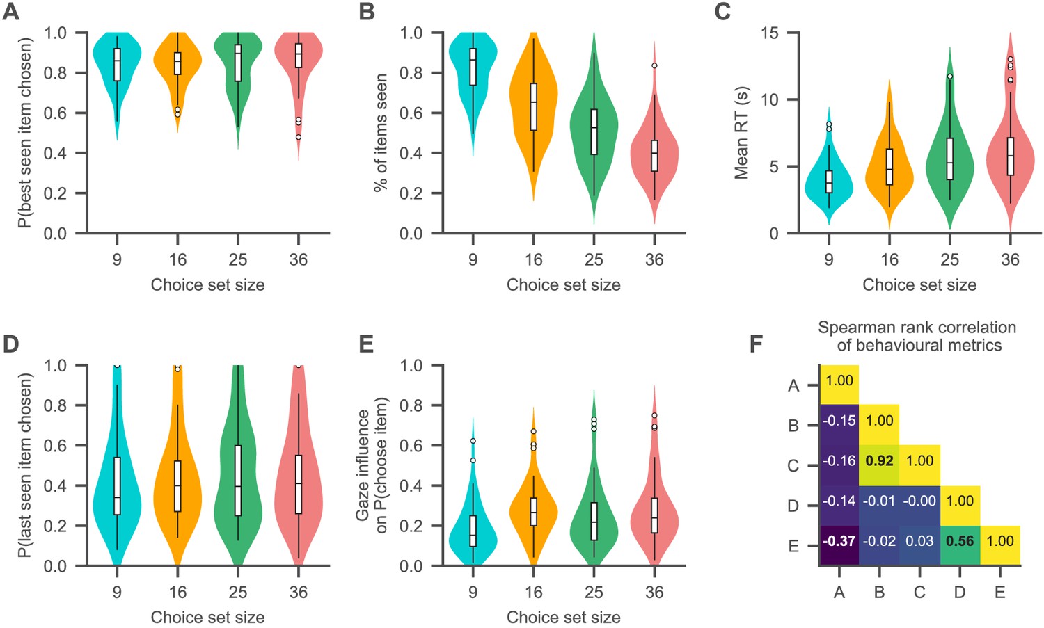
Choice psychometrics for each set size.
(A) The subjects were very likely to choose one of the highest-rated (i.e., best) items that they looked in all set sizes. (B, C) The fraction of items of a choice set that subjects looked at in a trial decreased with set size (B), while subjects’ mean RTs increased (C). (D) Subjects chose the item that they looked at last in a trial about half the time. (E) Subjects generally exhibited a positive association of gaze allocation and choice behaviour (as indicated by the gaze influence measure, describing the mean increase in choice probability for an item that is looked at longer than the others, after correcting for the influence of item value on choice probability; for details on this measure, see Qualitative model comparison). (F) Associations of the behavioural measures shown in (A–E) (as indicated by Spearman’s rank correlation). Correlations are computed by the use of the pooled subject means across the set size conditions. Correlations with p-values smaller than 0.01 (Bonferroni corrected for multiple comparisons: 0.1/10) are printed in bold font. For a detailed overview of the associations of the behavioural measures, see Figure 4—figure supplement 2. See the Qualitative model comparison section for the corresponding statistical analyses. For a detailed overview of the associations between the behavioural choice measures and individuals’ visual search, see Figure 4—figure supplement 1. Different colours in (A–E) represent the set size conditions. Violin plots show a kernel density estimate of the distribution of subject means with boxplots inside of them.
Figure 4—figure supplement 1
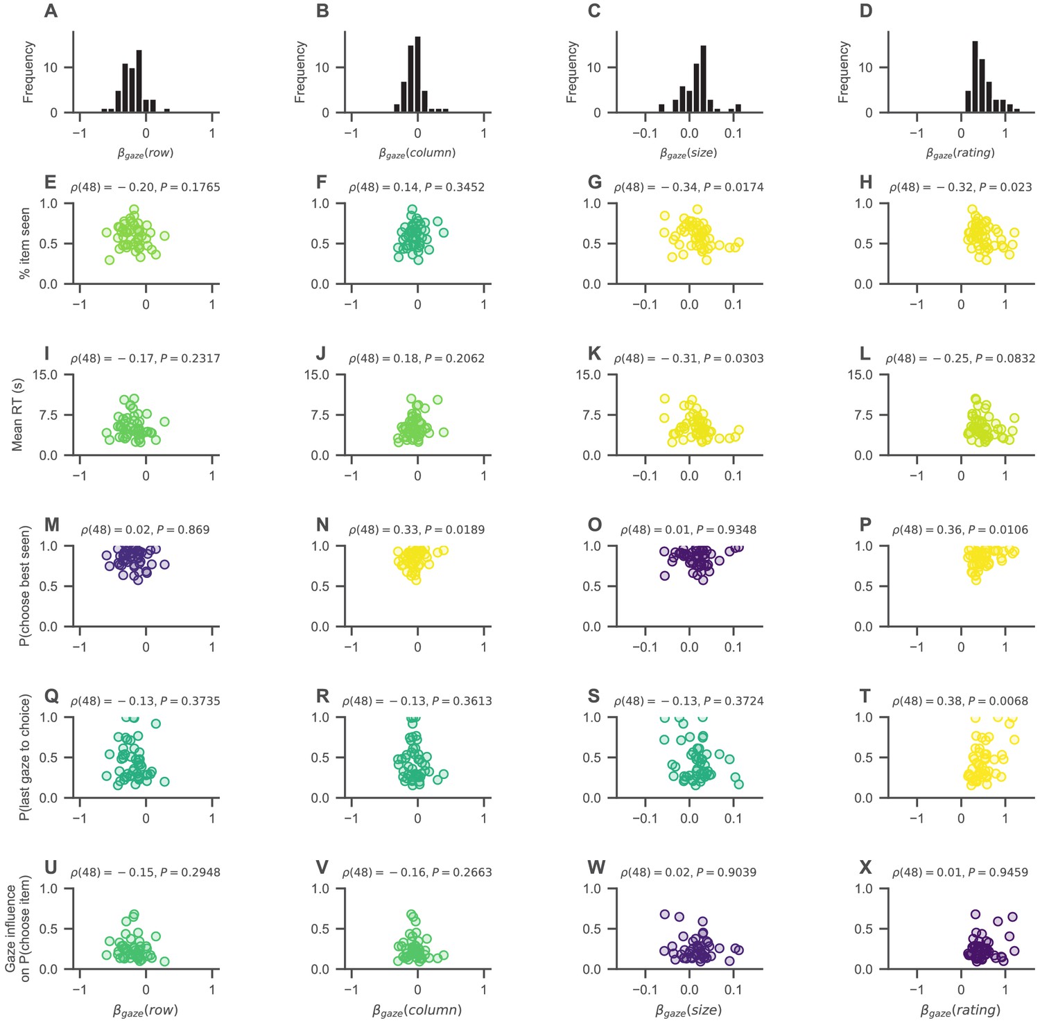
Association between the choice psychometrics presented in Figure 4A–E of the main text and a set of measures describing individuals’ visual search behaviour.
To quantify individuals’ visual search, we computed a mixed-effects regression model for each individual in the data, estimating how much the individual’s cumulative allocation of gaze to an item (measured as the fraction of trial time that the item was looked at) is influenced by the item’s attributes (namely, the item’s row and column position, size, and liking rating; for details on the item attributes, see the Materials and methods section of the main text) as well as the set size, resulting in one coefficient estimate (βgaze) for the influence of each item attribute and set size on the distribution of cumulative gaze. We then studied the relationship between the resulting regression estimate (βgaze; A–D) for each of the item attributes and each individual's pooled mean on the five behavioural choice metrics presented in Figure 4A–E of the main text (namely, the mean fraction of items looked at in a trial, mean RT, the probability of choosing the highest-rated seen item from a choice set, the probability of looking at the chosen item last, and the gaze influence measure). Spearman’s rank correlation coefficient (ρ) with p-value is reported for each association (E-X). Brighter yellow colours indicate smaller p-values. Scatter points indicate pooled subject means across the set sizes.
Figure 4—figure supplement 2
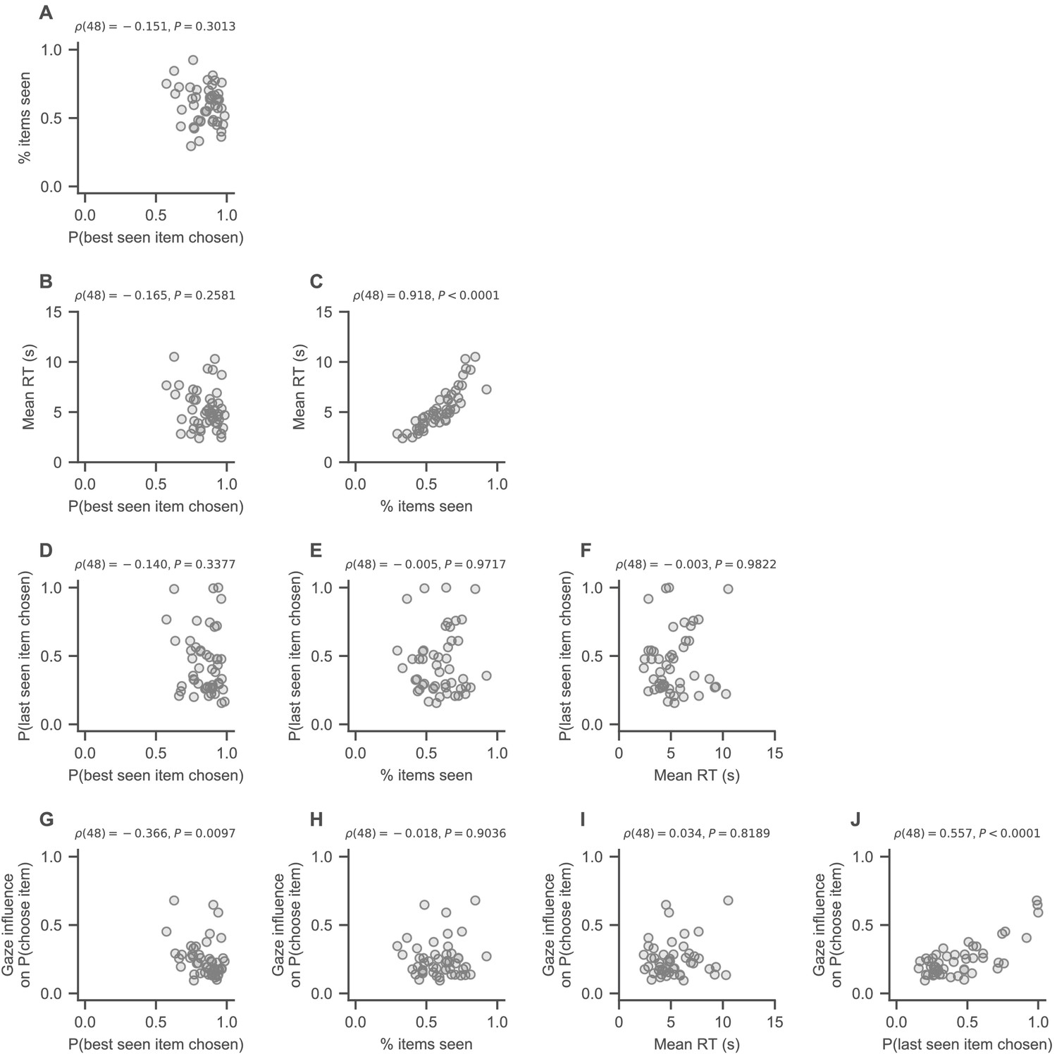
Detailed view of the associations of the choice psychometrics presented in Figure 4F of the main text.
Scatter points indicate pooled subject means across the set sizes. Spearman’s rank correlation coefficients (ρ) with corresponding p-values are reported for each association.
Figure 5 with 2 supplements
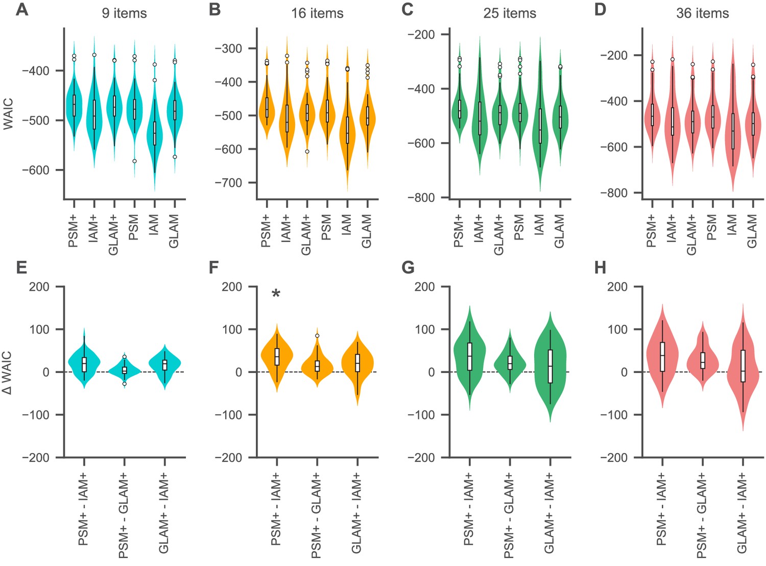
Relative model fit.
(A-D) Individual WAIC values for the probabilistic satisficing model (PSM), independent evidence accumulation model (IAM), and gaze-weighted linear accumulator model (GLAM) for each set size. Model variants with an active influence of gaze are marked with an additional ’+'. The WAIC is based on the log-score of the expected pointwise predictive density such that larger values in WAIC indicate better model fit. Violin plots show a kernel density estimate of the distribution of individual values with boxplots inside of them. (E–H) Difference in individual WAIC values for each pair of the active-gaze model variants. Asterisks indicate that the two distributions of WAIC values are meaningfully different in a Mann–Whitney U test with a Bonferroni adjusted alpha level of 0.0042 per test (0.05/12). See the Quantitative model comparison section for the corresponding statistical analyses. For an overview of the distribution of individual model parameter estimates, see Figure 5—figure supplement 1 and Supplementary files 1–3. For an overview of the results of a model recovery of the three model types, see Figure 5—figure supplement 2. Colours indicate set sizes.
Figure 5—figure supplement 1
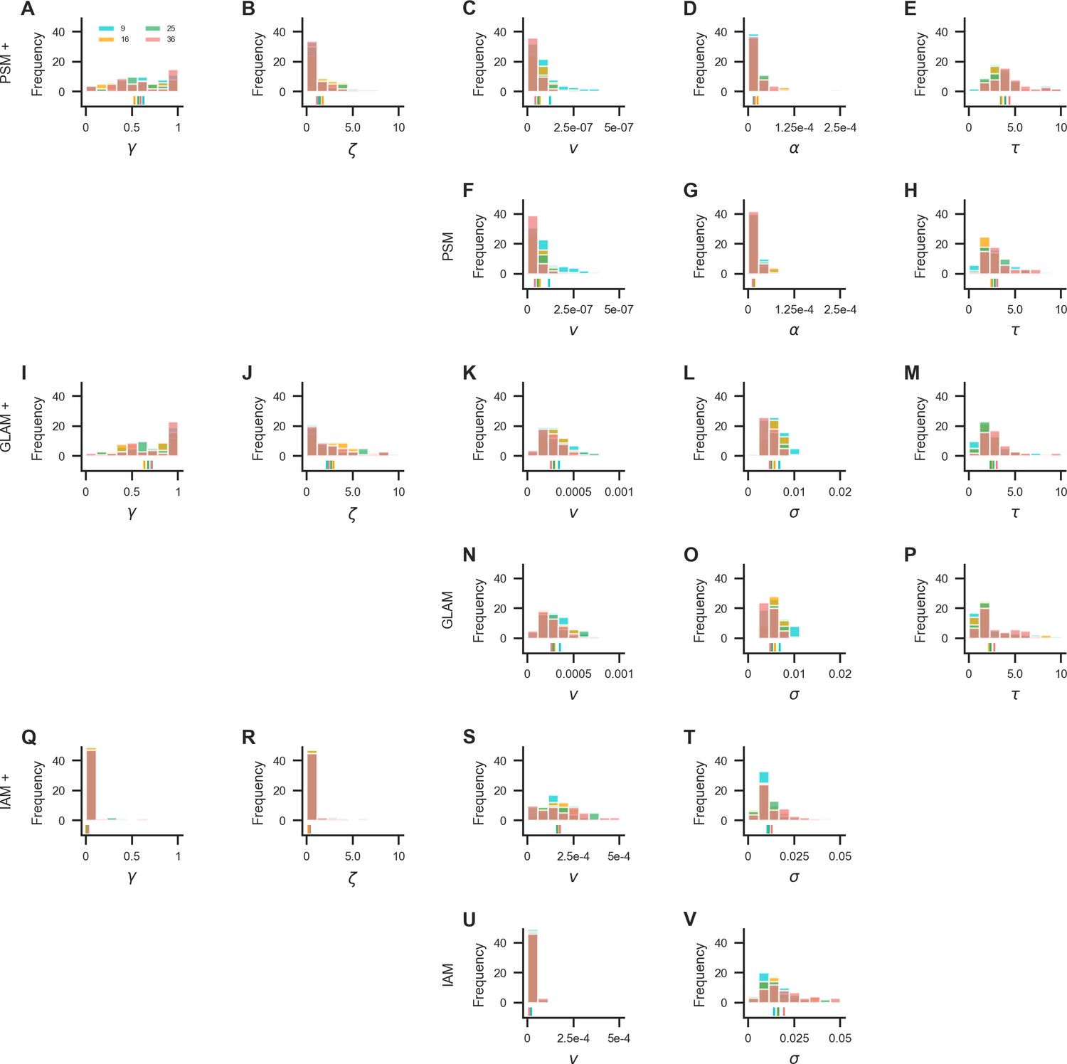
Parameter estimates from the in-sample fits of the probabilistic satisficing model (PSM; active-gaze variant: A–E, passive-gaze variant: F–H), GLAM (active-gaze variant: I–M, passive-gaze variant: N–P), and independent evidence accumulation model (IAM; active-gaze variant: Q–T, passive-gaze variant: U, V).
Colours indicate set sizes. Vertical lines on the x-axis indicate the mean parameter estimate in each set size. For a detailed overview of the mean parameter estimates per model and set size, see Supplementary files 1–3.
Figure 5—figure supplement 2
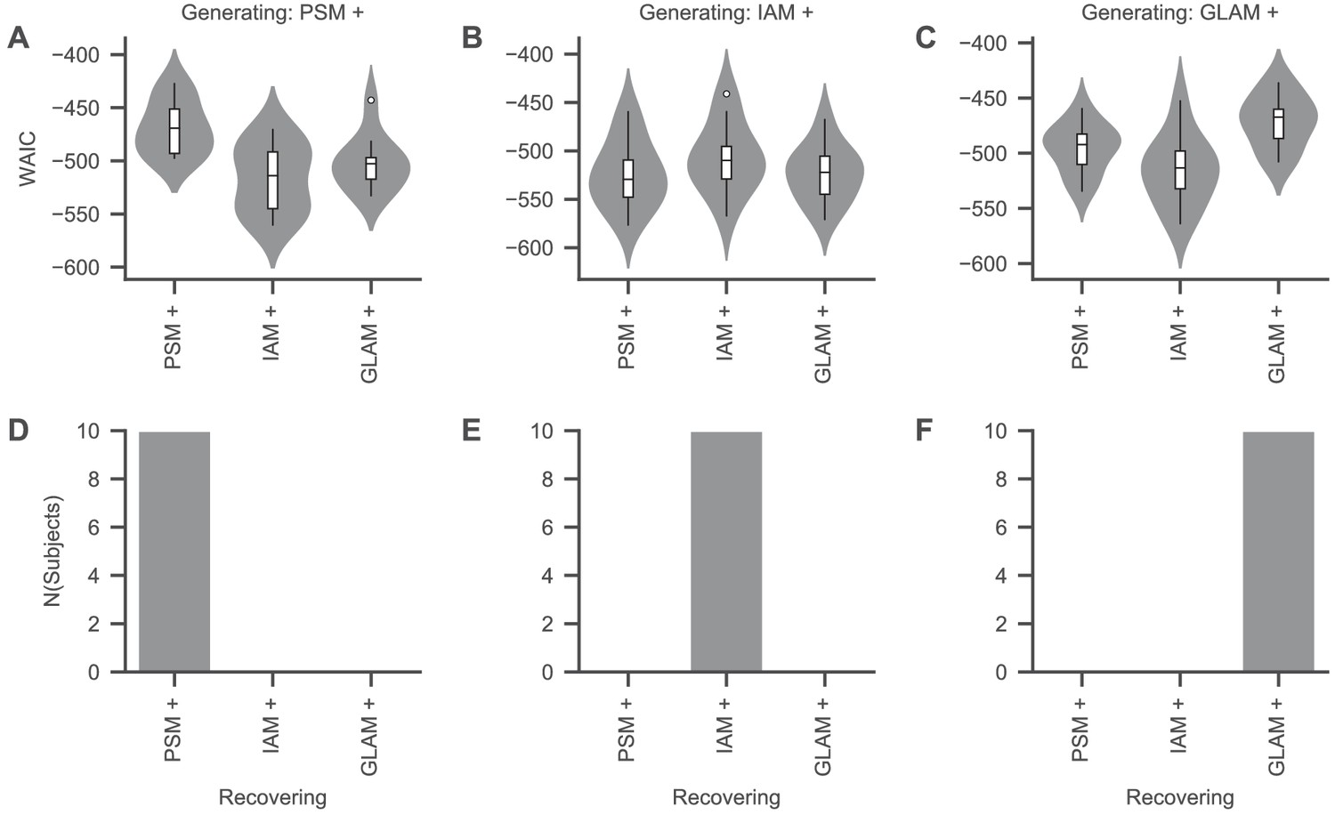
Model recovery.
The goal of this analysis was to determine whether the three models with an active account of gaze (PSM+, IAM+, and GLAM+; see the Materials and methods section of the main text) can be distinguished from one another in our dataset. Testing this is necessary to ensure that we can accurately identify the data-generating process. To test this, we selected 10 random subjects from our dataset and simulated choice and RT data for each of their nine-item trials (using the best-fitting individual parameters [Figure 5—figure supplement 1]). Subsequently, we fitted the three models to each simulated dataset and compared their fit by means of the widely applicable information criterion (WAIC; Vehtari et al., 2017) (A–C). The WAIC is based on the log-score of the expected pointwise predictive density such that larger values in WAIC indicate better model fit. Each model consistently best captured its own predictions (D–F), indicating that the three models can be distinguished from one another. For details on the model simulation and fitting procedures, see the Materials and methods section of the main text. Violin plots show a kernel density estimate of the distribution of individual values with boxplots inside of them.
Figure 6
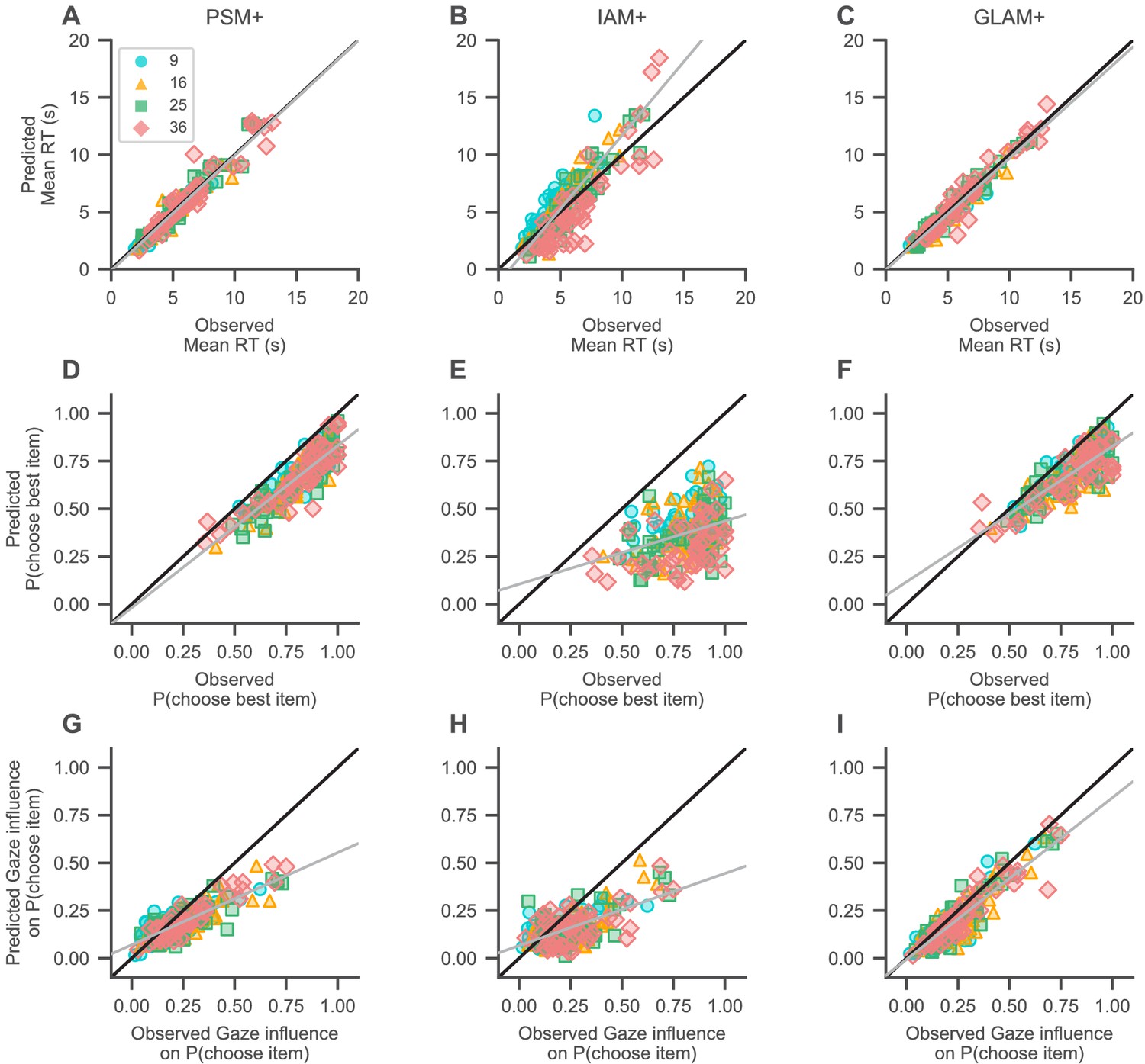
Absolute model fit.
Predictions of mean RT (A–C), probability of choosing the highest-rated (i.e., best) item (D–F), and gaze influence on choice probability (G–I; for details on this measure, see Qualitative model comparison) by the active-gaze variants of the probabilistic satisficing model (PSM+; A, G, D), independent evidence accumulation model (IAM+; B, E, H), and gaze-weighted linear accumulator model (GLAM+; C, F, I). (A–C) The PSM+ and GLAM+ accurately recover mean RT, while the IAM+ underestimates short and overestimates long mean RTs. (D–F) The PSM+ provides the overall best account of choice accuracy, followed by the GLAM+, and IAM+. (G–I) The PSM+ and IAM+ clearly underestimate strong influences of gaze on choice; the GLAM+ provides the best account of this association and only slightly underestimates strong influences of gaze on choice. Gray lines indicate mixed-effects regression fits of the model predictions (including a random intercept and slope for each set size) and black diagonal lines represent ideal model fit. Model predictions are simulated using parameter estimates obtained from individual model fits (for details on the fitting and simulation procedures, see Materials and methods). See the Quantitative model comparison section for the corresponding statistical analyses. Colours and shapes represent different set sizes, while scatters indicate individual subjects.
Figure 7
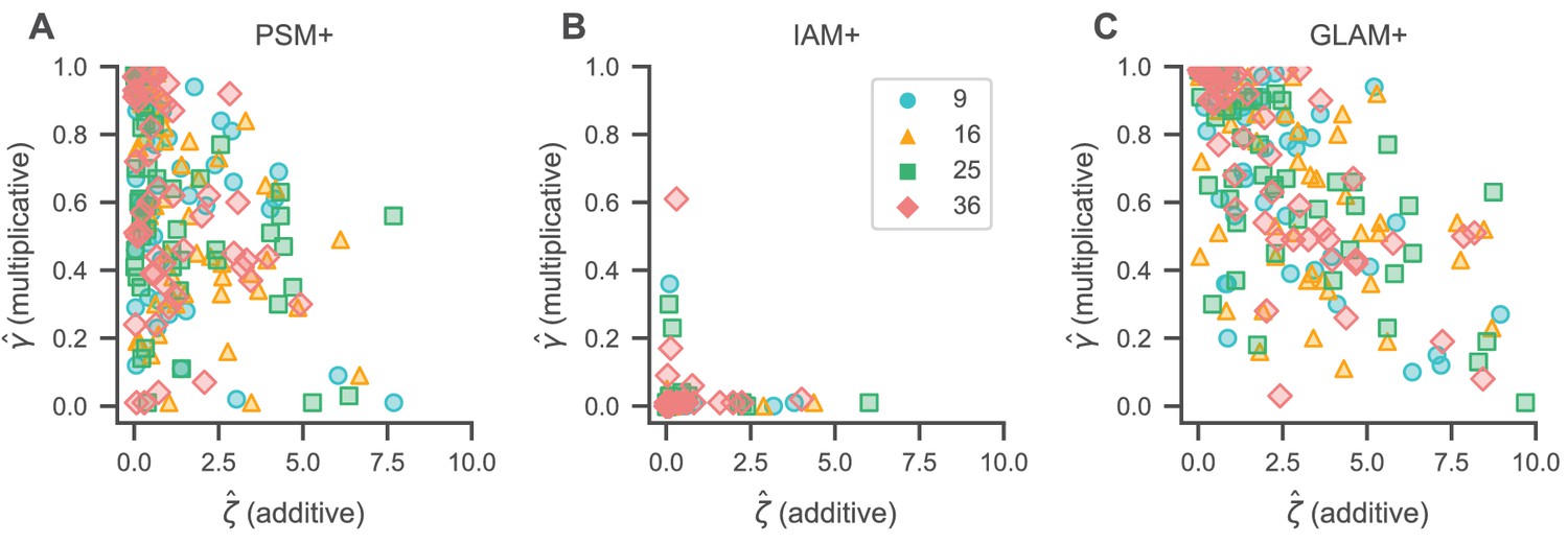
Gaze bias estimates.
Association of individual γ (multiplicative) and ζ (additive) gaze bias estimates for the PSM+ (A), IAM+ (B), and GLAM+ (C). γ estimates generally decrease with increasing ζ estimates for the PSM+ (A) and GLAM+ (C), indicating that individuals with stronger additive gaze biases generally also exhibit stronger multiplicative gaze biases. We did not find any association of γ and ζ estimates for the IAM+ (B). See the Gaze bias mechanism section for the corresponding statistical analyses. Colours and shapes represent different set sizes, while scatters indicate individual subjects.
Videos
Animation 1
Exemplar visual search trajectory for choice sets with 9 alternatives.
The video shows the visual search trajectory over the choice screen for one example trial . The current gaze position is indicated by a white box, while the choice is indicated by a red box. For better visibility, gaze durations have been increased by a factor of two.
Animation 2
Exemplar visual search trajectory for choice sets with 16 alternatives.
The video shows the visual search trajectory over the choice screen for one example trial. The current gaze position is indicated by a white box, while the choice is indicated by a red box. For better visibility, gaze durations have been increased by a factor of two.
Animation 3
Exemplar visual search trajectory for choice sets with 25 alternatives.
The video shows the visual search trajectory over the choice screen for one example trial. The current gaze position is indicated by a white box, while the choice is indicated by a red box. For better visibility, gaze durations have been increased by a factor of two.
Animation 4
Exemplar visual search trajectory for choice sets with 36 alternatives.
The video shows the visual search trajectory over the choice screen for one example trial. The current gaze position is indicated by a white box, while the choice is indicated by a red box. For better visibility, gaze durations have been increased by a factor of two.
Additional files
-
Supplementary file 1
Mean parameter estimates of the probabilistic satisficing model with active (PSM+) and passive (PSM) account of gaze in the decision process for each set size.
The probabilistic satisficing model has five parameters, determining the additive () and multiplicative () gaze bias effects on its cached value, the influence of cached value () and time () on its stopping probability, and the sensitivity of its softmax choice rule (). Note that the high mean value of for the active-gaze variant in the set size with 16 items is driven by one outlier (Figure 5—figure supplement 1D).
- https://cdn.elifesciences.org/articles/57012/elife-57012-supp1-v1.docx
-
Supplementary file 2
Mean parameter estimates of the independent evidence accumulation model with active (IAM+) and passive (IAM) account of gaze in the decision process for each set size.
The independent evidence accumulation model has four parameters, determining its additive () and multiplicative () gaze bias effects and its general accumulation speed () and noise ().
- https://cdn.elifesciences.org/articles/57012/elife-57012-supp2-v1.docx
-
Supplementary file 3
Mean parameter estimates for the gaze-weighted linear accumulator model with active (GLAM+) and passive (GLAM) account of gaze in the decision process for each set size.
The GLAM variant used in this work has five parameters, determining its additive () and multiplicative () gaze bias, its general accumulation speed () and noise () as well as the sensitivity of the scaling of the relative decision signals (τ).
- https://cdn.elifesciences.org/articles/57012/elife-57012-supp3-v1.docx
-
Transparent reporting form
- https://cdn.elifesciences.org/articles/57012/elife-57012-transrepform-v1.pdf
Download links
A two-part list of links to download the article, or parts of the article, in various formats.
Downloads (link to download the article as PDF)
Open citations (links to open the citations from this article in various online reference manager services)
Cite this article (links to download the citations from this article in formats compatible with various reference manager tools)
Uncovering the computational mechanisms underlying many-alternative choice
eLife 10:e57012.
https://doi.org/10.7554/eLife.57012


