How to measure and evaluate binding affinities
- Department of Biochemistry, Stanford University, United States
- Department of Chemical Engineering, Stanford University, United States
- Stanford ChEM-H, Stanford University, United States
Figures
Figure 1 with 2 supplements

Assessment of published KD values for RNA-binding proteins.
We analyzed 100 papers reporting KD or ‘apparent KD’ values of RNA/protein interactions. Measurements were evaluated based on two criteria: demonstrating equilibration (horizontal axis) and controlling for titration (vertical axis). Detailed criteria are described in Materials and methods, and the source data are provided in Supplementary file 1. The right column includes predominantly studies that used ITC and SPR, techniques that inherently record binding progress over time (24/30 in this column). The fraction of studies that varied time to demonstrate equilibration in non-ITC/SPR experiments is considerably smaller (6 of the 76 papers that did not exclusively use ITC or SPR, or <10%).
Figure 1—figure supplement 1
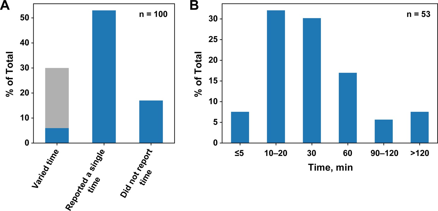
Survey of incubation times for published equilibrium dissociation constants.
(A) Percentages of publications that did or did not report and vary the incubation time. The light gray portion of the first column indicates the studies using SPR and ITC, techniques in which time is varied by default. (B) Incubation times in papers that reported a single time.
Figure 1—figure supplement 2
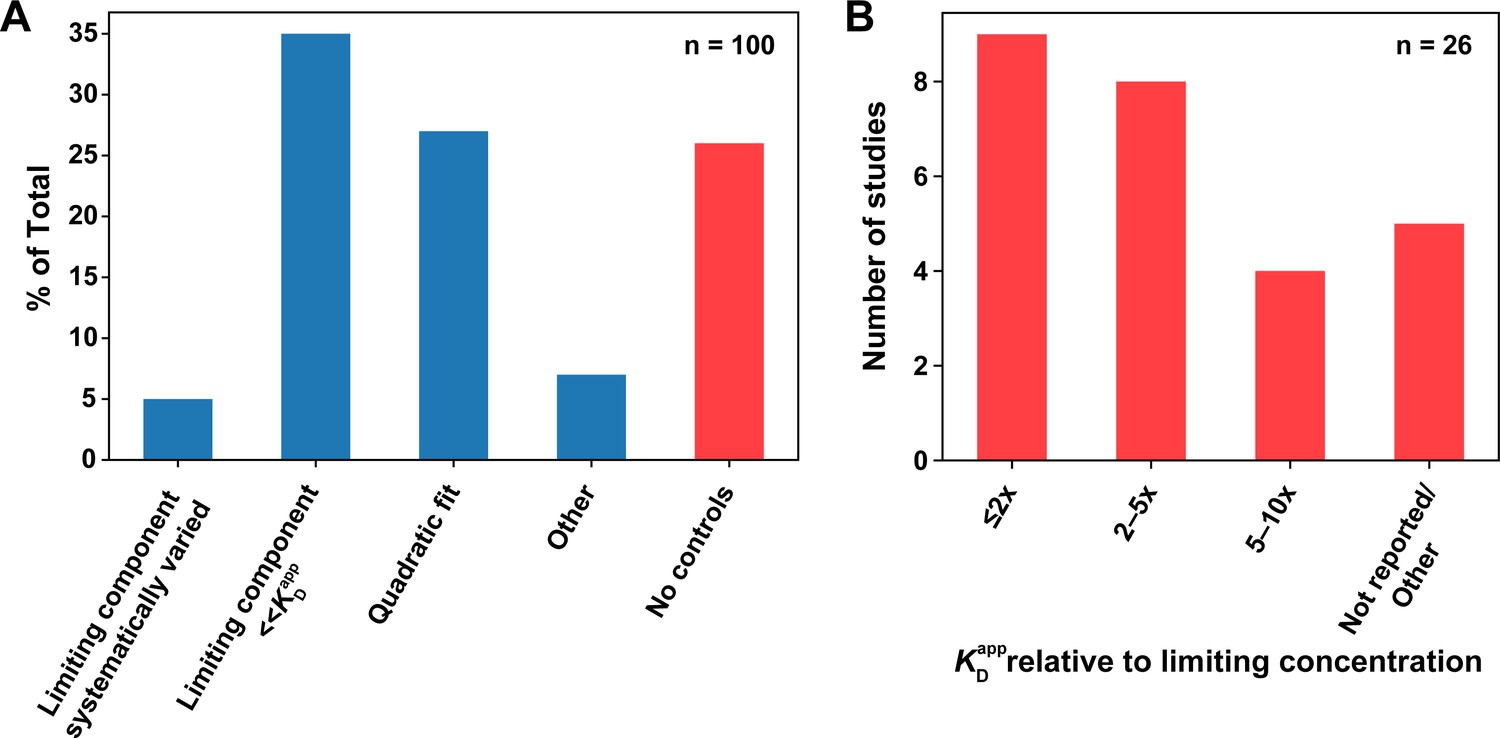
Survey of titration controls in published binding studies.
(A) Percentages of publications that did (blue) or did not (red) control for titration effects. The first category includes studies that systematically varied the limiting component concentration to rule out titration. Studies that reported using an appropriate concentration regime or analysis methods to minimize the effects of titration (second and third column, respectively) were considered titration controlled; nevertheless, we emphasize the importance of performing and reporting the control experiments described herein, instead of relying on concentrations alone (see section 'Avoid the titration regime'). The ‘Other’ category (n = 7) includes a study that reported KD values as upper limits, recognizing possible titration (n = 1), and studies that only used SPR (n = 6), where the concentration of the immobilized species is difficult to estimate, but mass transport is typically controlled for or accounted for during analysis, as indicated in most surveyed studies. (B) Breakdown of studies that did not report controlling for titration. The first three columns denote studies that assumed negligible concentration of the limiting component in their analysis; however, the reported concentrations and KD values were inconsistent with this assumption, with the ratio of the lowest measured KD value to the limiting component concentration indicated. The ‘Not reported/Other’ category includes studies that did not report the limiting component concentration (n = 4), or used the quadratic equation in a titration regime (limiting component concentration in >1000-fold excess over the KD), incompatible with reliable KD determination (n = 1; see below).
Figure 2
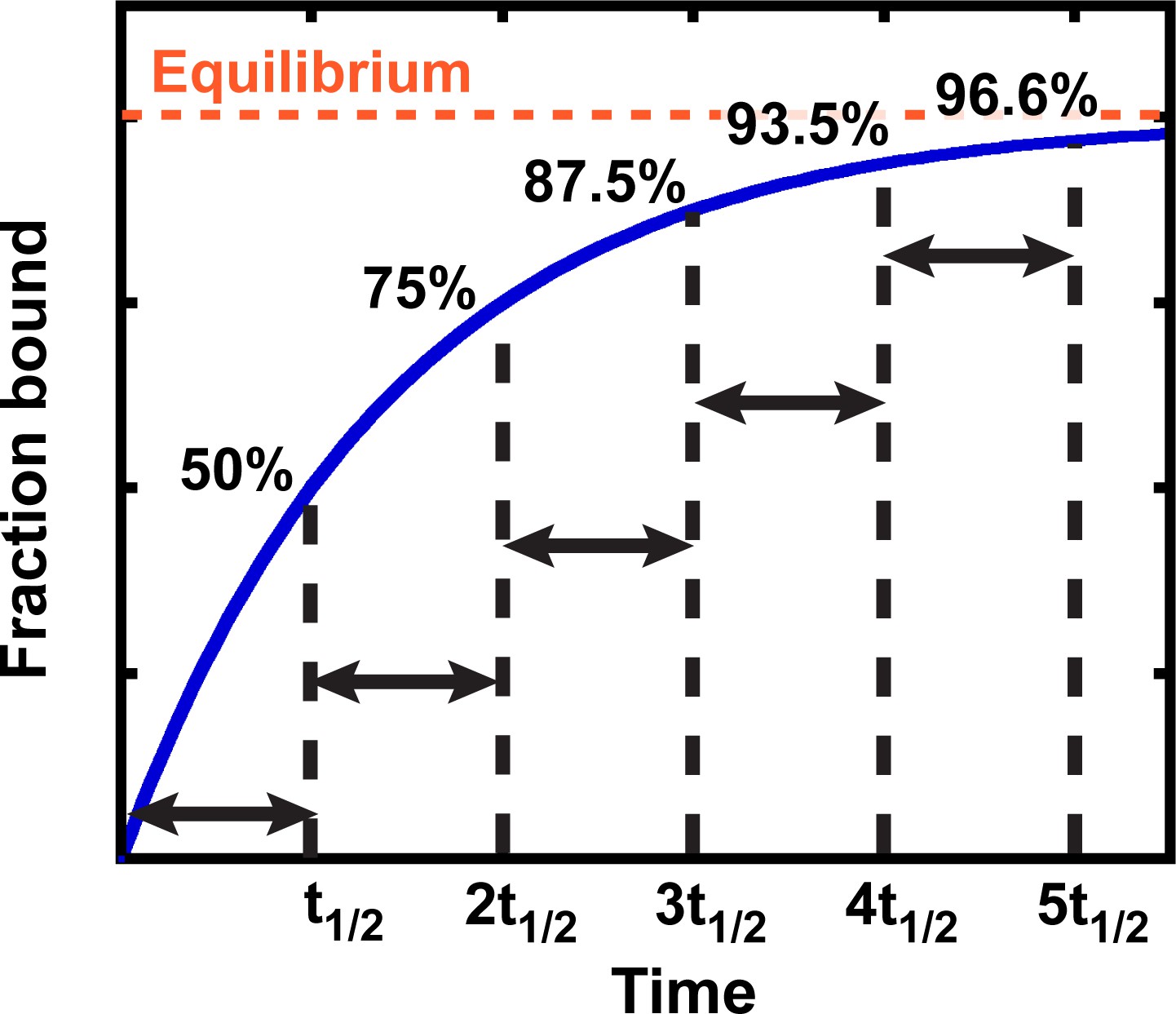
Exponential kinetics used to estimate the time needed for binding equilibration.
Arrows indicate reaction half-life t1/2. Fraction bound is defined by the equation = .
Figure 3
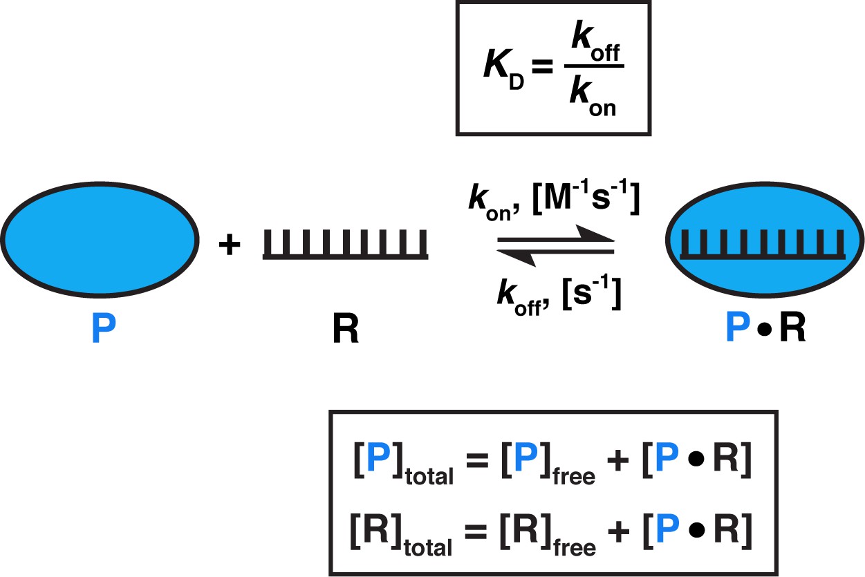
Model for one-step, non-cooperative, 1:1 binding between two molecules.
Protein (P) binding to an RNA (R) molecule is shown for illustrative purposes.
Figure 4 with 1 supplement
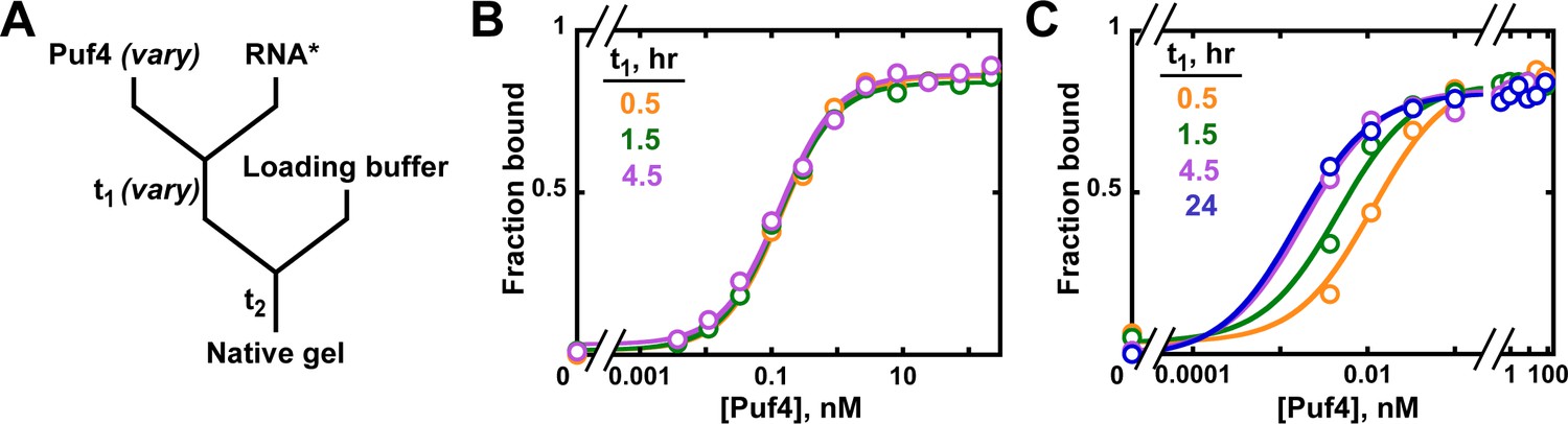
Establishing equilibration in affinity measurements.
(A) Mixing scheme. RNA*: labeled RNA (here—5´-terminally labeled with 32P). In addition to varying equilibration time t1 (main text), the time and conditions between adding the loading buffer and loading (t2) are controlled (see Appendix 2—note 2). (B, C) Concentration dependence of Puf4 binding at 25°C (B) and at 0°C (C) after different incubation times. Data were collected at protein concentrations greater than or equal to the concentration of labeled RNA (0.002–0.016 nM, indicating the lower and upper limit of labeled RNA concentration; see section 'Avoid the titration regime' and Appendix 2—note 4).
Figure 4—figure supplement 1
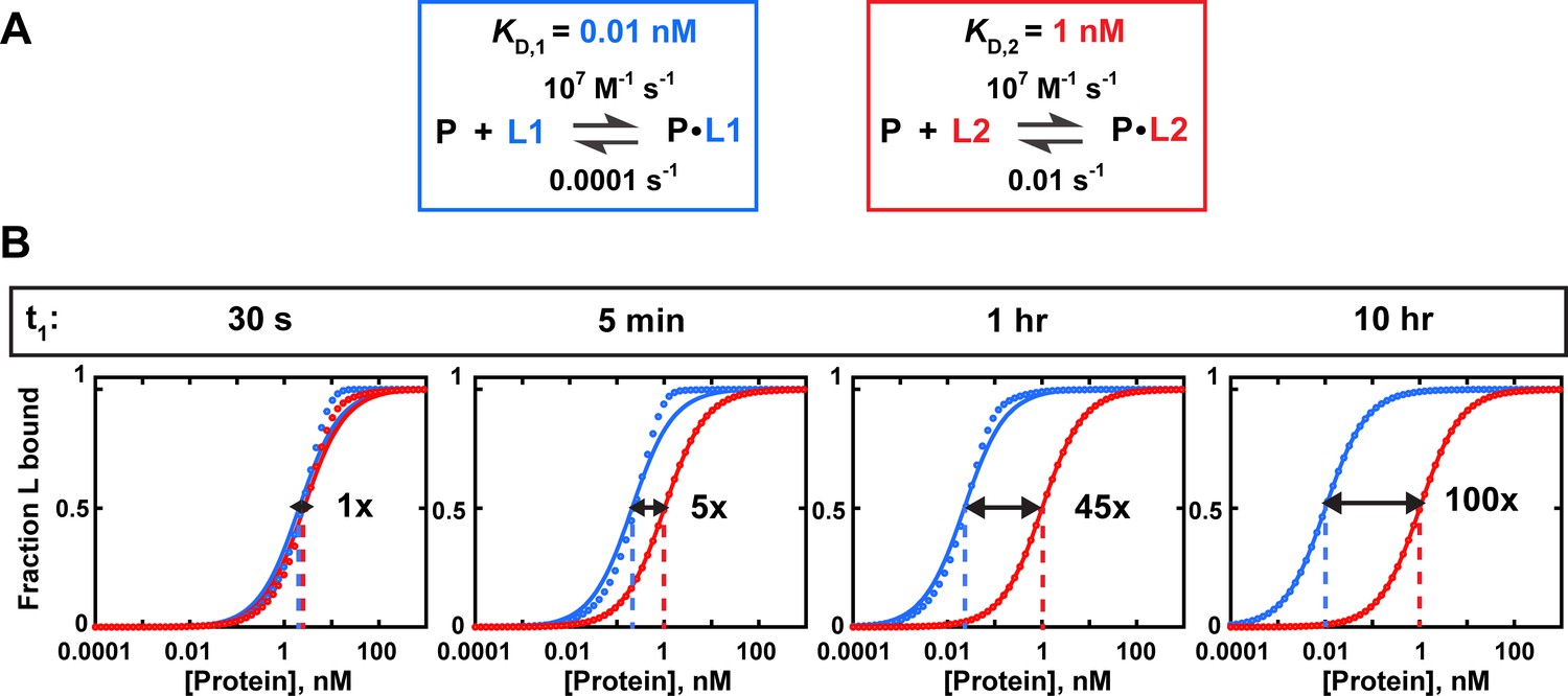
Insufficient equilibration times can lead to incorrect determination of relative affinities.
(A) Binding parameters for protein (P) interactions with two ligands, L1 and L2. The dissociation rate constant (koff) for L1 is 100-fold lower than for L2, such that L1 requires much longer to equilibrate than L2 (Equation 2). (B) Simulated binding data for L1 and L2 with varying incubation times (t1). The binding to each ligand is measured individually with trace amounts of L1 (blue) or L2 (red). Solid lines are fits to an equilibrium binding equation (Equation 4b), with dashed lines indicating the protein concentration at which half of the ligand is bound. Because equilibration of L1 binding is not complete until t1 = 10 hr (while L2 equilibration only takes ~5 min), the observed relative affinity ((rel) = /) is time-dependent and underestimates the true specificity if the incubation time is shorter than ~10 hr. Arrows and numbers indicate (rel) values at each time point. Note the systematic deviations of the simulated data from the fit curve in cases where equilibrium has not been reached. The presence of such deviations in experimental data indicates the need for additional controls to establish equilibration and rule out titration.
Figure 5 with 5 supplements
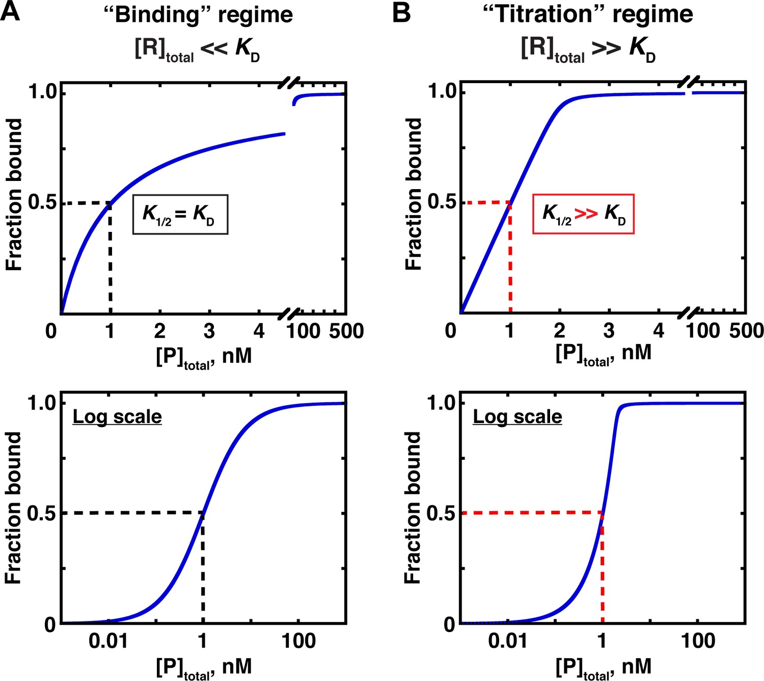
Two concentration regimes.
(A) Binding curve for the model in Figure 3 in the ‘binding’ regime—that is, the trace binding partner concentration ([R]total) is much lower than KD and much lower than [P]total (Equation 4b). Here, the KD is simply the protein concentration at which half of the RNA is bound (K1/2, here corresponding to 1 nM). The same simulated binding curve is shown in linear (top) and log (bottom) plots, as both are useful and common in the literature. (B) Binding curve in the ‘titration’ regime, simulated for an interaction with a KD value of 0.01 nM and an [R]total of 2 nM. Although the K1/2 value in this example is identical to the example in Part A, here it does not equal KD, instead exceeding the real KD value by 100-fold.
Figure 5—figure supplement 1
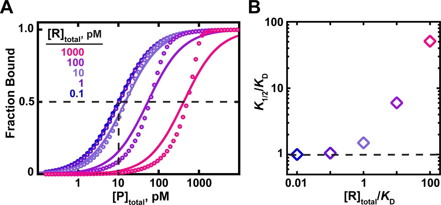
The effects of RNA (ligand) concentration on observed binding.
(A) Circles indicate simulated data for an interaction with a KD = 10 pM in the presence of RNA concentrations ranging from 100-fold below to 100-fold above the KD. Curves indicate fits of the simulated data to a hyperbolic equation (Equation 4b). For RNA concentrations ≤10-fold below the KD, the data are well explained by a hyperbolic fit, and the protein concentration at which half-saturation occurs (K1/2; indicated with dashed lines for the 0.1 pM RNA curve) is consistent with the KD. Higher RNA concentrations lead to increasing deviations from a hyperbolic fit and have increasing K1/2 values as the RNA concentration increases. (B). The relationship between the observed K1/2 enhancement over the true KD (‘K1/2/KD’) and the total RNA concentration relative to KD (‘[R]total/KD’). K1/2 values were derived from the simulated data in part A using Equation 4b.
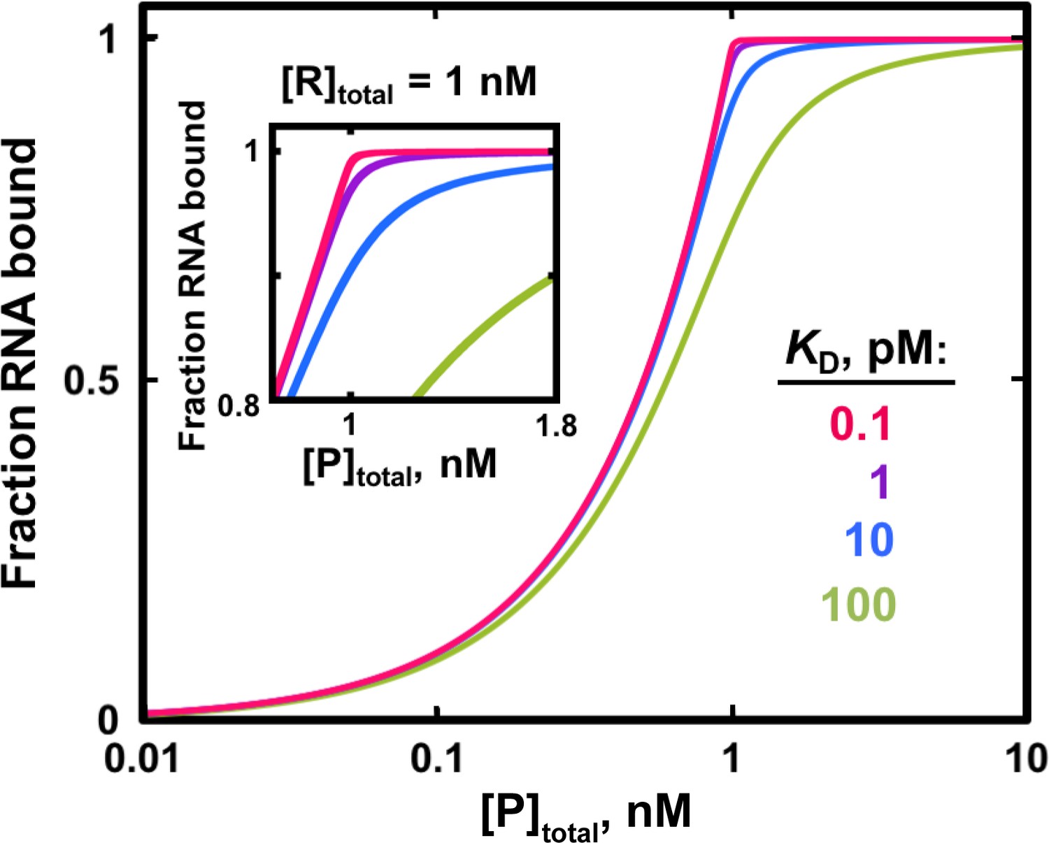
Figure 5—figure supplement 2
Fit to the quadratic binding equation becomes less sensitive to differences in KD when the RNA concentration is in large excess over the KD.
Simulated binding curves for RNA/protein interactions of varying affinities are shown in the presence of 1 nM labeled RNA. In this example, KD = 1 pM (1000-fold lower than [R]total) would be essentially impossible to distinguish from KD = 0.1 pM (10,000-fold lower than [R]total) and from even lower KD values because of the nearly identical binding curves. To accurately measure KD = 10 pM (100-fold lower than [RNA]) it would be critical to have a large number of data points in the narrow protein concentration range that distinguishes this curve from weaker and especially from stronger binders (inset).
Figure 5—figure supplement 3
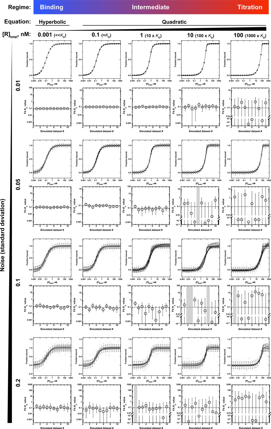
Application of the hyperbolic (Equation 4b) and quadratic (Equation 5) binding equations to simulated binding data with increasing noise levels.
All binding curves are for an RNA-protein interaction with a KD of 0.1 nM, measured in the presence of different RNA concentrations (0.001–100 nM) and with increasing levels of random noise in the fraction bound (standard deviation of 0.01–0.2). Ten datasets were simulated per condition and noise level and were individually fit to Equation 4b (leftmost column) or Equation 5 (the remaining columns) to determine the KD. The binding curves are shown as black lines, and the overlaid white circles indicate the expected fractions bound if the data were not affected by noise, with error bars indicating the standard deviation. The fit KD values for each of the 10 simulated datasets are shown below each set of binding curves, and the error bars indicate the 95% confidence intervals (CIs) of the KD. Gray bars indicate that the KD could not be determined from a quadratic fit. CIs that extend beyond the axis limits indicate that the lower limit of the KD was not defined. Note that with increasing noise and increasing RNA concentration the KD values derived from the quadratic fits become increasingly poorly constrained, particularly the lower CIs. By contrast, using the binding regime and Equation 4b to fit the data (leftmost column) consistently yields well-defined KD values, even with substantial noise.
Figure 5—figure supplement 4
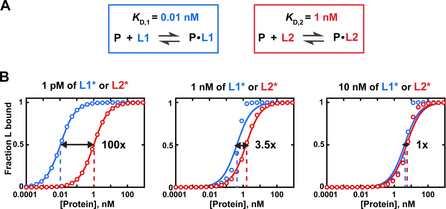
Effects of trace binding partner concentration on apparent relative affinities.
(A) Affinities of protein P for ligands L1 and L2. (B) Simulated equilibrium binding curves. Binding to each ligand is measured individually with different concentrations of labeled ligand (L1* or L2*). Solid lines are fits to Eq. 4b, with dashed lines indicating the protein concentration at which half of the ligand is bound (corresponding to KD in Equation 4b). Arrows and numbers indicate apparent KD(rel) values at each concentration of L ((rel) = /; with and derived using Equation 4b). There is a pronounced dependence of apparent relative affinity on ligand concentration if [L] is not much lower than the KD for the most tightly bound ligand among the ligands being compared. If sufficiently low ligand concentrations are not accessible, Equation 5 should be used and results may be less reliable (see section 'Avoid the titration regime' of main text).
Figure 5—figure supplement 5

Concentration regimes that do not (A) and do (B) affect the determination of equilibrium binding constants.
(A) Labeled RNA concentration is much lower than KD ([R*]total << KD; binding regime). (B) Labeled RNA concentration is greater than KD ([R*]total > KD; intermediate regime). In parts (A) and (B), concentrations are indicated schematically by the number of RNA (R*, red), protein (P, light blue) molecules and RNA-protein complexes (P●R*) shown. In each case, protein concentration is varied (6, 18, 54, 400 arbitrary units), and KD equals 18 (in the same units). The total RNA concentration is 4 (A) and 36 (B). (C) Protein concentration dependence of binding in each of the above regimes. In the binding regime (green, [R*]total << KD from part A), the protein concentration at which half of the RNA is bound corresponds to the KD. In contrast, in the intermediate regime (purple, [R*]total > KD from part B), a greater protein concentration is required to achieve half-saturation (40 vs. 18 arbitrary units). The discrepancy would further increase with higher RNA concentrations, as shown in Figure 5—figure supplement 1. We can understand the origin of this discrepancy as follows. In part (A), the RNA concentration (red) is below the KD value and below the protein concentration (blue), such that the free concentration of the protein is essentially unchanged after RNA binding at both saturating (complete binding of RNA) and sub-saturating protein concentrations. Changing the RNA concentration in this regime would not change the fraction of RNA bound at a given total protein concentration, as long as the [R*]total << KD condition remains met. On the contrary, in part (B), the RNA concentration exceeds the dissociation constant (KD) and is high enough that a large fraction of the total protein is bound by RNA. Thus, the free protein concentration, which determines the extent of binding according to Equation 4a, is depleted and can no longer be approximated by the total protein concentration in Equation 4b to obtain an accurate KD value. On the molecular scale, the lowered free protein results in less binding. Consequently, for a given KD, more protein is required to achieve half-saturation at higher RNA concentration than with a trace concentration of RNA. Intuitively, at a concentration of RNA that is greater than KD there simply isn’t enough protein to occupy half the RNA when the total protein concentration is equal to KD.
Figure 6
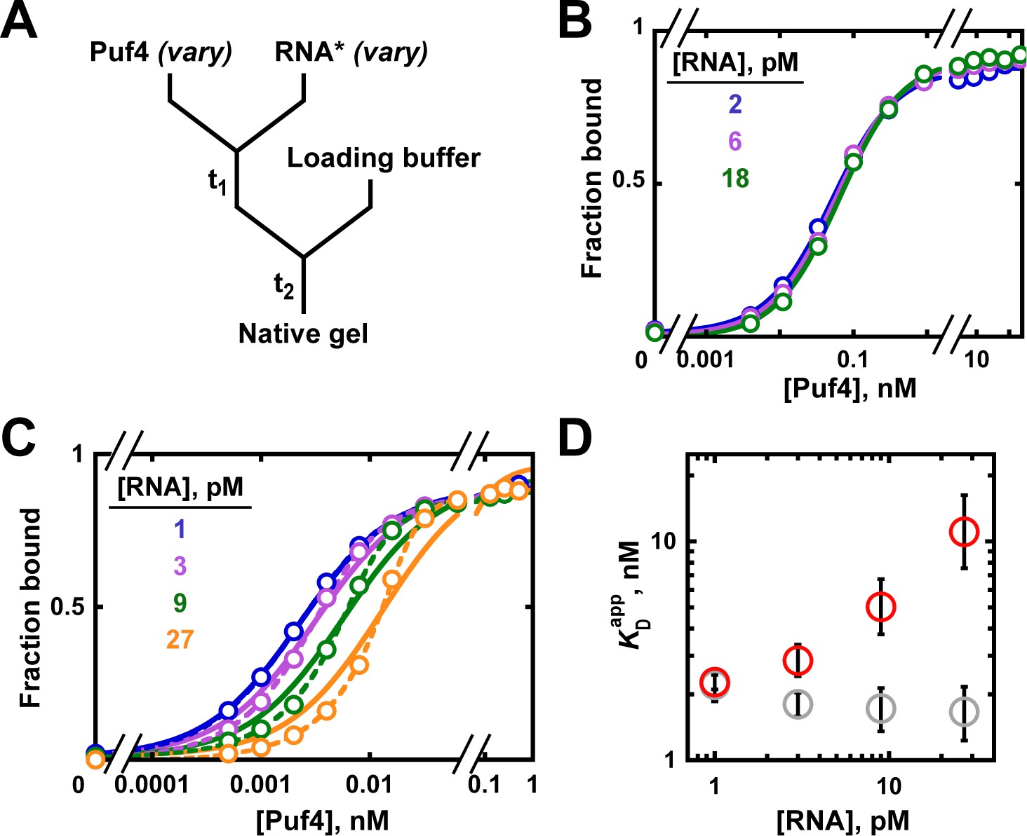
Varying the concentration of the 'trace' binding partner.
(A) Mixing scheme, as in Figure 4A but now with a series of labeled RNA concentrations. (B) Puf4 binding to different concentrations of 32P-labeled RNA at 25°C. For simplicity, only the lower limits of RNA concentration are indicated; the corresponding upper limits were 15–140 pM RNA (see Materials and methods and Appendix 2—note 4). Incubation time t1 was 0.5 hr, as established in Figure 4B. (C) Puf4 binding to different concentrations of 32P-labeled RNA at 0°C. Lower limits of labeled RNA concentration are indicated. Incubation time t1 was 40 hr. Note that these data are not fit well by Equation 4b, which assumes [R*]total << KD (solid lines). Quadratic fits, which do not assume negligible RNA concentration, are shown in dashed lines (Equation 5). (D) Effect of RNA concentration on apparent KD () at 0°C. Red symbols indicate values from a hyperbolic fit (Equation 4b and solid lines in C) and grey symbols indicate values from fits to the quadratic equation (Equation 5). The error bars denote 95% confidence intervals, as determined by fitting the data to the indicated equation in Prism 8.
Figure 7 with 1 supplement
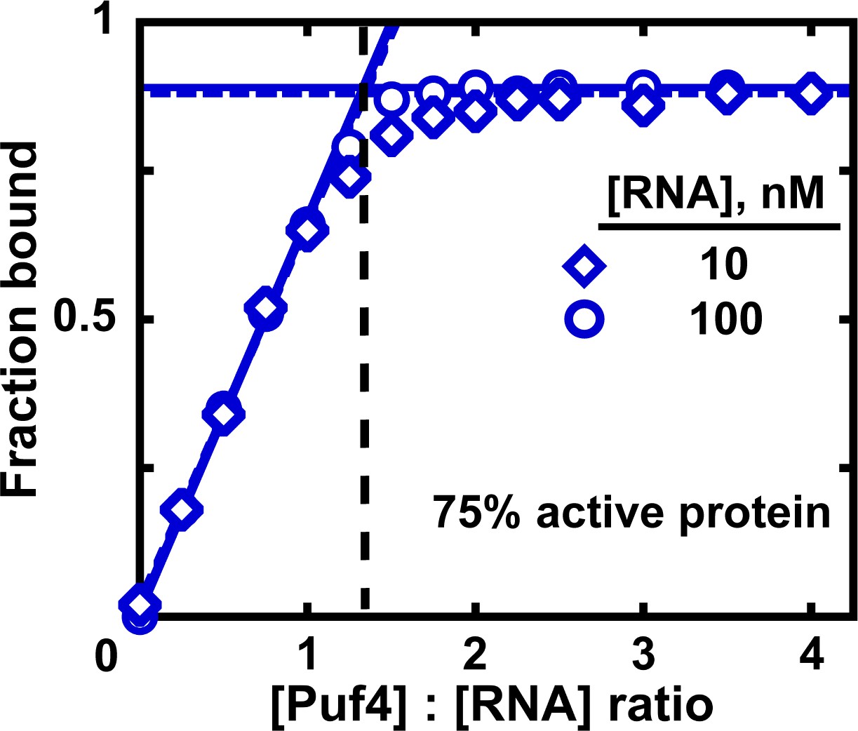
Measuring the fraction of active protein by titration.
The fraction of active protein is derived from the breakpoint, that is, the intersection of linear fits to the low and high-Puf4 concentration data. See Figure 7—figure supplement 1 for an alternative strategy using Equation 5.
Figure 7—figure supplement 1
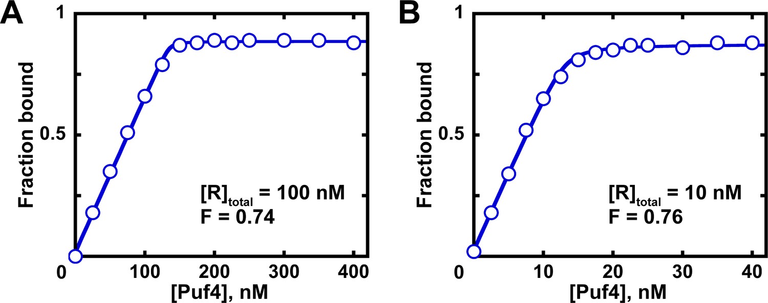
Determination of the fraction of active protein from a quadratic fit.
Fits of titration data at 100 nM (A) and 10 nM (B) RNA to the quadratic equation are shown. The quadratic equilibrium-binding equation (Equation 5) was modified to include a term for the active protein fraction.
(8)
A and O correspond to the amplitude and Y axis offset, respectively; F is the fraction of active protein; was constrained to the known RNA concentration (10 or 100 nM); here, the value was constrained to the known affinity (Table 2). The last constraint is optional, as the value contributes minimally to the fit at these high RNA concentrations and because the exact value may not yet be known at the time of measuring the active protein fraction. The fit fractions of active protein (F) are almost identical to those determined from linear fits of the same data in Figure 7 (~0.75).
Appendix 1—figure 1
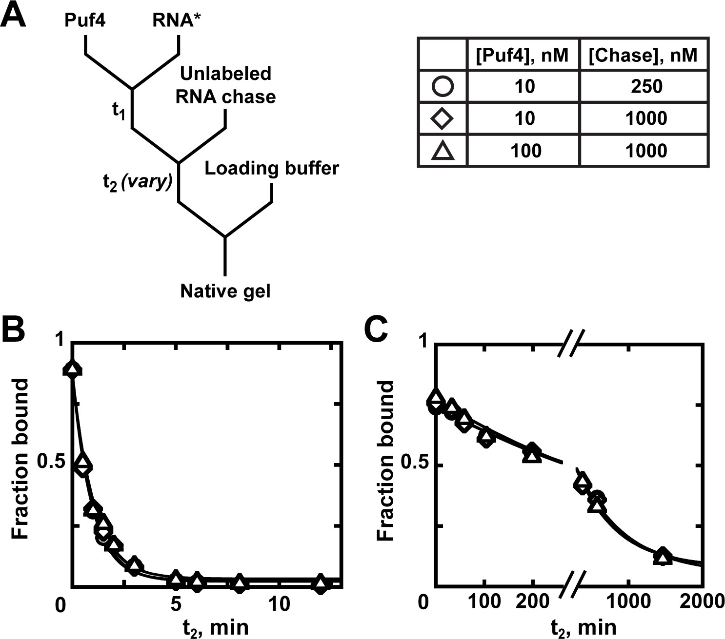
Kinetics of Puf4 dissociation.
(A) Mixing scheme for measuring the dissociation rate constant. After equilibration of a saturating or near-saturating concentration of Puf4 protein with a trace concentration of labeled RNA (t1), a large excess of unlabeled RNA is added, with concomitant dilution of the binding reaction to prevent rebinding after dissociation. (B–C) Time dependence of Puf4 dissociation from its consensus RNA at 25°C (C; koff = (0.014 ± 0.003) s−1) and at 0°C (D; koff = (2.92 ± 0.17) × 10−5 s−1).
Appendix 1—figure 2
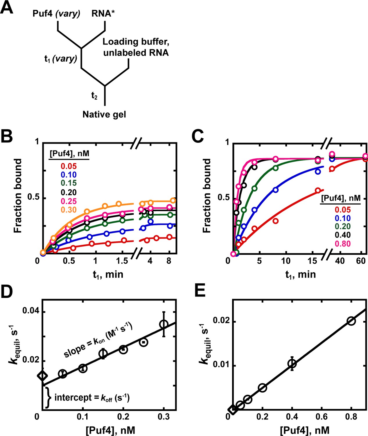
Kinetics of Puf4/RNA association.
(A) Mixing scheme for measuring association rate constants. (B, C) Time dependence of Puf4 association to its consensus RNA at 25°C (B) and 0°C (C). (D, E) Determination of kon from the slope of the Puf4 concentration dependence of equilibration rate constants in parts B and C, respectively (circles). The koff values from Appendix 1—figure 1 are also shown (diamonds) to illustrate the correspondence between the y-intercept and koff (Equation 1). Panels D and E show results from two and one independent experiments, respectively (error bars in E correspond to averages from measurements at two different labeled RNA concentrations).
Appendix 3—figure 1
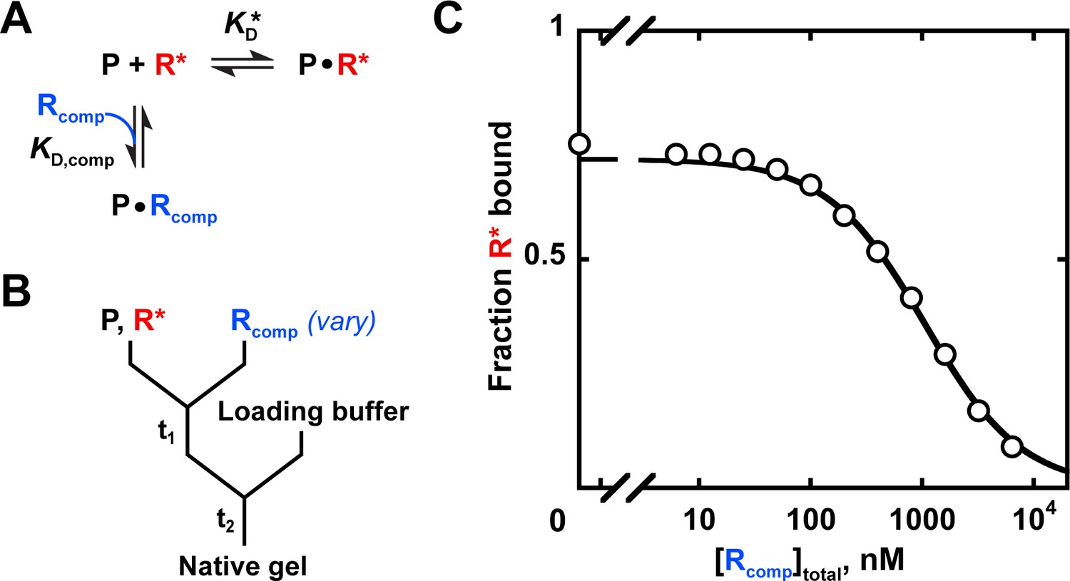
Measuring binding affinity by competition.
(A) Competitive binding reaction scheme. R*: labeled RNA ligand; Rcomp: unlabeled competitor RNA; : protein affinity for R*; : protein affinity for Rcomp. (B) Mixing scheme for a competition measurement. (C) Competition between the U1C point mutant of the Puf4 consensus (Rcomp = CGUAUAUUA) and the labeled consensus RNA (R*= 32P-AUGUGUAUAUUAGU). The data were fit to the following equation (Lin and Riggs, 1972; Weeks and Crothers, 1992):
(9)
A indicates the maximum amplitude, constrained to the fit amplitude of the R* binding curve that is measured in parallel by a direct binding experiment (A = 0.89 for Puf4 binding to R*). O is the y axis offset (background). [R*]total was constrained to the lower limit of the labeled RNA concentration. was constrained to Puf4 affinity for the labeled RNA, as determined by direct measurement in the same experiment (0.105 nM, after accounting for active protein fraction of 75%). [P]total was 0.45 nM, after accounting for active protein fraction. The fit value was 204 nM. Incubation times of 10, 30, and 110 min gave consistent values (190–210 nM), as did lowering the protein concentration by three-fold (180 nM). Equation 9 is applicable only for . For other cases see Wang, 1995.
Appendix 4—figure 1
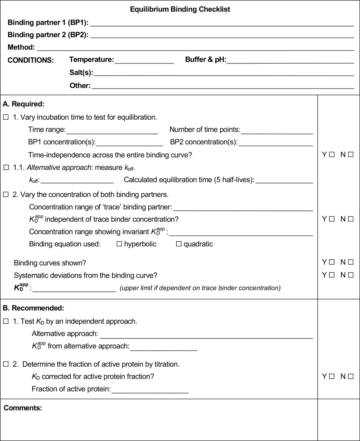
Equilibrium binding checklist template.
Appendix 4—figure 2
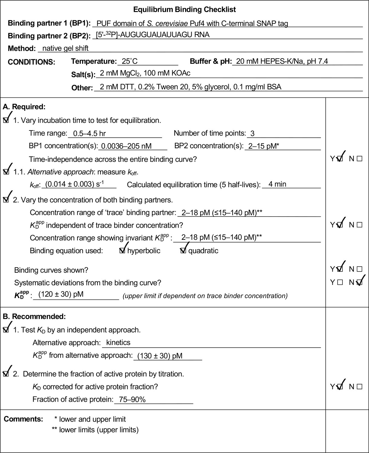
Example of a completed equilibrium binding checklist based on Puf4/RNA binding at 25°C.
Appendix 4—figure 3
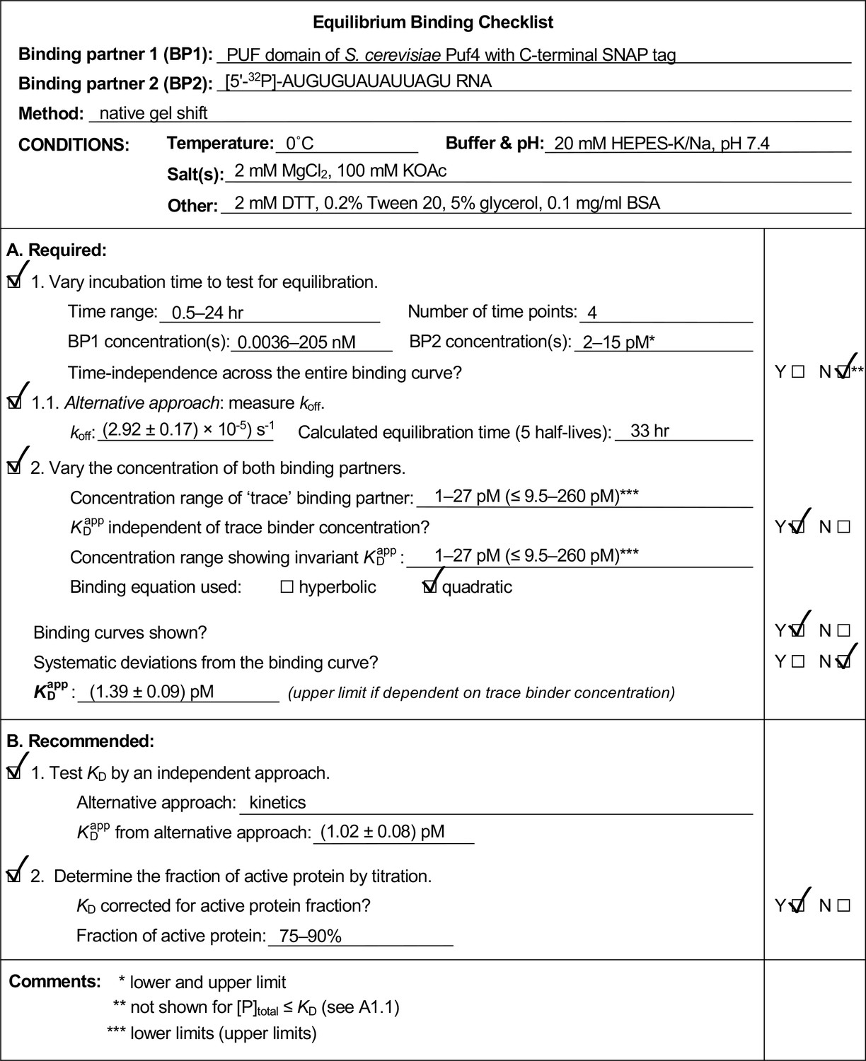
Example of a completed equilibrium binding checklist based on Puf4/RNA binding at 0°C.
Tables
Table 1
Equilibration times (tequil) for different affinities and association rate constants.
| KD | kon, M−1 s−1 | tequil* | |
|---|---|---|---|
| sec | hr | ||
| 1 µM | 108 | 0.04 | |
| 106 | 4 | ||
| 103 | 1 | ||
| 1 nM | 108 | 40 | |
| 106 | 1 | ||
| 103 | 1000 | ||
| 1 pM | 108 | 10 | |
| 106 | 1000 | ||
| 103 | 1,000,000 | ||
-
*tequil was calculated as five half-lives: tequil = 5t1/2 = 5 × 0.693/kequil, where kequil = koff = KD × kon (Equation 2 and Figure 3).
Table 2
Summary of equilibrium and kinetic measurements of Puf4 affinity.
| Equilibrium* | Kinetic | ||||
|---|---|---|---|---|---|
| Temperature,°C | KD(hyperbolic), pM | KD(quadratic), pM | kon, M−1s−1* | koff, s−1 | KD (=koff/kon), pM |
| 0 | ≤1.7 | 1.39 ± 0.09 | (2.85 ± 0.14)×107 | (2.92 ± 0.17)×10−5 | 1.02 ± 0.08 |
| 25 | 120 ± 30 | 120 ± 30 | (1.04 ± 0.14)×108 | 0.014 ± 0.003 | 130 ± 30 |
-
*The values have been normalized by active protein fraction (75–90%). KD(hyperbolic) and KD(quadratic) refer to values derived from fits to Equation 4b and Equation 5, respectively. Errors are defined in Materials and methods.
Additional files
-
Supplementary file 1
Literature survey of 100 RNA/protein binding studies.
- https://cdn.elifesciences.org/articles/57264/elife-57264-supp1-v2.xlsx
-
Supplementary file 2
Literature survey of CRISPR nuclease binding studies, representative of high-affinity interactions.
- https://cdn.elifesciences.org/articles/57264/elife-57264-supp2-v2.xlsx
-
Transparent reporting form
- https://cdn.elifesciences.org/articles/57264/elife-57264-transrepform-v2.docx
Download links
A two-part list of links to download the article, or parts of the article, in various formats.
Downloads (link to download the article as PDF)
Open citations (links to open the citations from this article in various online reference manager services)
Cite this article (links to download the citations from this article in formats compatible with various reference manager tools)
How to measure and evaluate binding affinities
eLife 9:e57264.
https://doi.org/10.7554/eLife.57264


