Figures and data in Mesoscopic-scale functional networks in the primate amygdala

Figures
Tables
Additional files

5 figures, 1 table and 6 additional files

Figures

Figure 1

Download asset Open asset

Behavioral setup and example average traces across all trials on each of the 16 contacts.

All trials were separated by a 3–4 s inter-trial interval (ITI) and preceded by a visual fixation cue presented at the center of a monitor in front of the animal. If the monkey successfully fixated on the cue, the cue was removed and a single stimulus from one of the three sensory modalities (visual, tactile, auditory) was presented. All trials were followed by a brief delay (0.7–1.4 s) before a small consistent amount of juice was delivered. The color code of the peri-event LFP activity corresponds to the estimated location of the recording electrode within the nuclei of the amygdala. The lines with alternating colors refer to contacts located within 200 µm of an anatomical boundary between nuclei. ME = medial, magenta; CE = central, green; AB = accessory basal, yellow; BA = basal, cyan; LA = lateral, orange; non-amygdala contacts are colored black.

Figure 2

Download asset Open asset

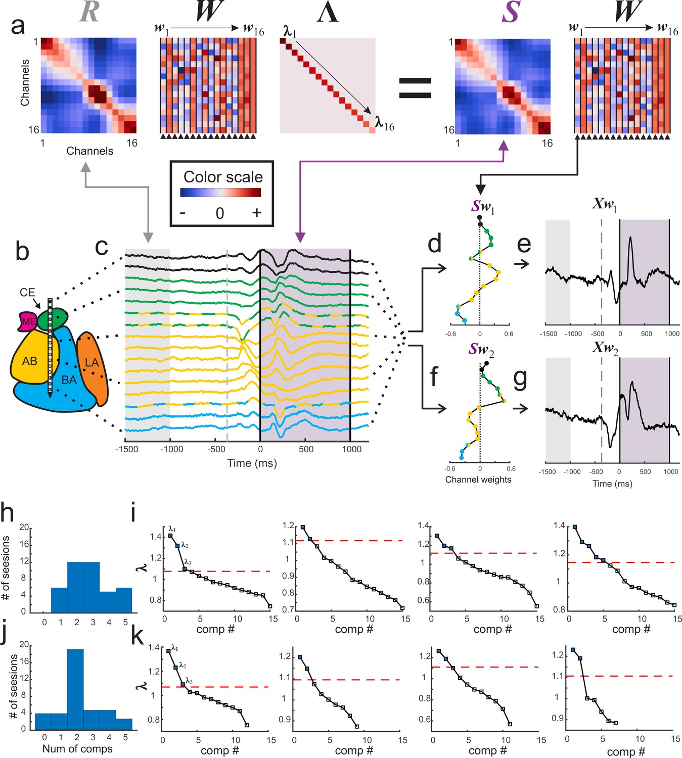
Visualization of GED.

(a) The elements of the equation for generalized eigendecomposition (RWΛ = SW), where R and S are 16x16 covariance matrices (corresponding to the 16 contacts) derived from baseline and stimulus activity respectively. These contact covariance matrices were generated for each trial and then averaged over trials (see Materials and methods). The columns in the W matrix (highlighted by the arrowheads below the plot) contain the eigenvectors. Each eigenvector from the matrix can be written as w_n (indicated by the w₁ → w₁₆ above the plots). The diagonal matrix of eigenvalues is represented by Λ. The individual eigenvalues are denoted by λ₁→λ₁₆ shown along the diagonal. A general color scale for the heatmap images is shown under the left side of the equation. (b) MRI-based reconstruction of recording sites in this session. (c) The average peri-stimulus LFP for each contact (color convention is the same as in Figure 1). Light gray shading represents the baseline period and the gray dotted line denotes fixspot onset (note that these data are aligned to stimulus onset; the baseline and fixspot indicators shown here are for illustrative purposes only). The purple shading marks stimulus delivery. Note that the data in (c) are contained in a time-by-contacts matrix (represented by X in subsequent equations). (d) Example of the component map associated with the largest eigenvalue (created by multiplying the stimulus covariance matrix with an eigenvector and termed Sw₁). (e) The component time series associated with this eigenvalue. This time series (represented as Xw₁) is created by multiplying the LFP data matrix (i.e., X) with the eigenvector in the first column of the (W) matrix (w₁). (**f, g**) the same as for (d) and (e) but associated with the second largest eigenvalue. (h) Histogram of the number of significant components per session when including all contacts regardless of location (i.e., within or outside of the amygdala). (i) Scree plots of the eigenvalues derived from GED from four example sessions when all contacts were included in analysis regardless of location. In the scree plots, the points above the dotted line correspond to the significant eigenvalues. (j) Histogram of the number of significant components per session when only amygdala contacts were included in the analysis. (k) Scree plots of the eigenvalues from the same sessions in (i) but only using amygdala contacts. Note that decreasing the number of contacts decreases the number of total components that GED is able to extract. This does not always result in decreases in the number of significant components (left two panels); however, small (right middle) and occasionally large (far right) decreases in the number of significant components were observed when removing non-amygdala contacts from the analysis.

Figure 3 with 1 supplement

Download asset Open asset

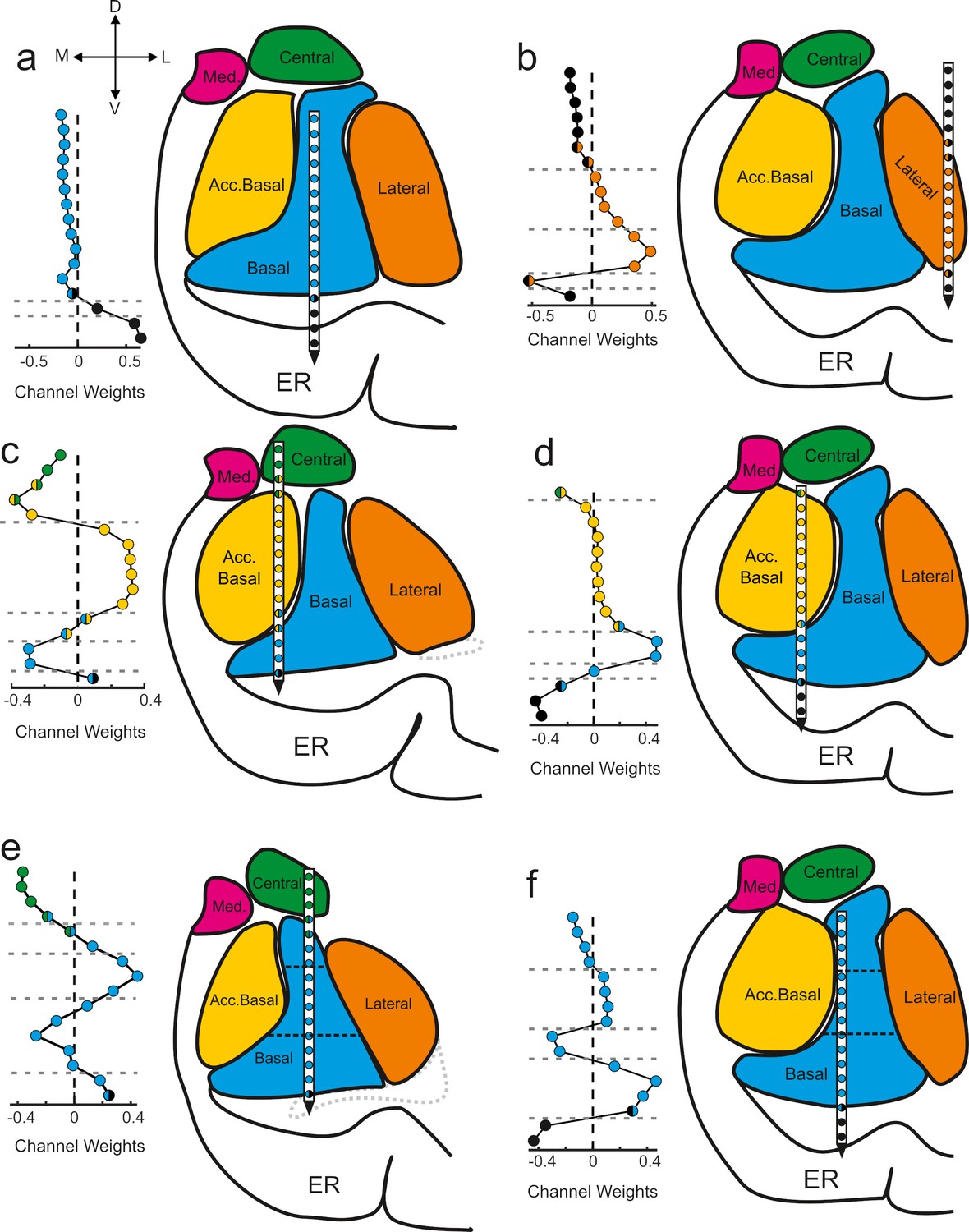
Components map onto anatomical boundaries.

Six examples of how component maps (left) match the MRI-based reconstruction of the electrode array positions (right). On each component map the x axis corresponds to the weight calculated for each contact (i.e., see Sw in Figure 2) of the V-probe and the y axis lists the contacts. In each panel, the colors of the contact weights match their estimated nuclear locations following the same convention as in previous figures. Gray dotted lines in the component map plots denote change points in the contact weights that statistically separate groups of contacts based on their coactivity patterns (see Methods). Ventricles are contoured in light gray dotted lines. Med = medial nucleus; Acc. basal = accessory basal nucleus; ER = entorhinal cortex. (**a–b**) Examples of large transitions in contact weights at boundaries between the amygdala and surrounding tissue, particularly on the ventral contacts. (**c–d**) Examples of component maps in which the statistical clustering (dotted horizontal lines) match the geometry of the nuclear boundaries. (**e–f**) Two examples of component maps in which the statistical boundaries correspond to known subnuclear divisions of the basal nucleus.

Figure 3—figure supplement 1

Download asset Open asset

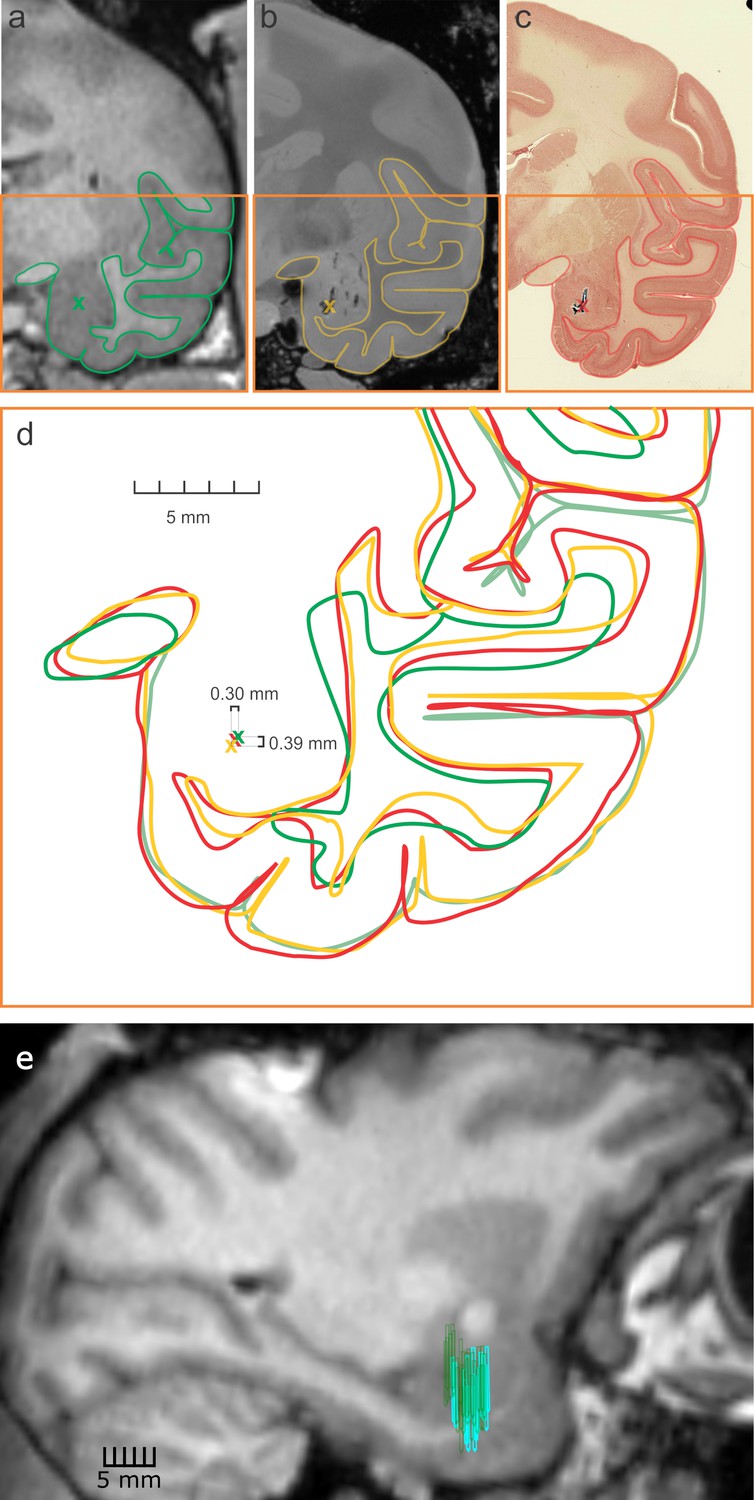
Histological verification of electrode placement.

(a) Coronal slice from a 3T MRI scan of the right hemisphere of the brain of monkey B at the location of a dye injection into the amygdala. The MRI scan was taken after the surgical implant of the recording chamber. The green X indicates the predicted site of a cell stain injected immediately preceding euthanasia and perfusion (4% PFA) of the brain. The targeting of the injection site and the estimated locations of the contacts were both calculated relative to the same stereotaxic coordinates used for initial implantation of the recording chamber. (b) Coronal slice from an ex vivo, high-resolution 7T MRI. The scan was performed on the brain of monkey B ten weeks after perfusion and provided a more detailed visualization of the injection prior to histological processing. The gold X indicates the position of the dye injection. Note that electrode tracks can be seen dorsal and lateral to the injection site. (c) Histological verification of injection site estimates on a neutral-red stain. The red X indicates the position of the dye injection. (d) The estimated locations of the dye injection site along with the boundaries of major temporal lobe structures (contained in the orange boxes in **a–c**) from the three images were overlaid. The numbers around the injection site reconstructions (i.e., the X’s) indicate the distances between the centers of the farthest separated sites (green and gold) in the dorsal-ventral (0.39 mm) and medial-lateral (0.30 mm) axes. These distances show that even when taking the largest differences in estimated injection location, the dorso-lateral and ventral-medial error is less than the space between two contacts on the V-probe. (e) Projection of all estimated array positions from recordings in monkeys B (cyan) and F (green) onto a single sagittal slice from a 3T MRI scan of the brain of monkey B.

Figure 4 with 1 supplement

Download asset Open asset

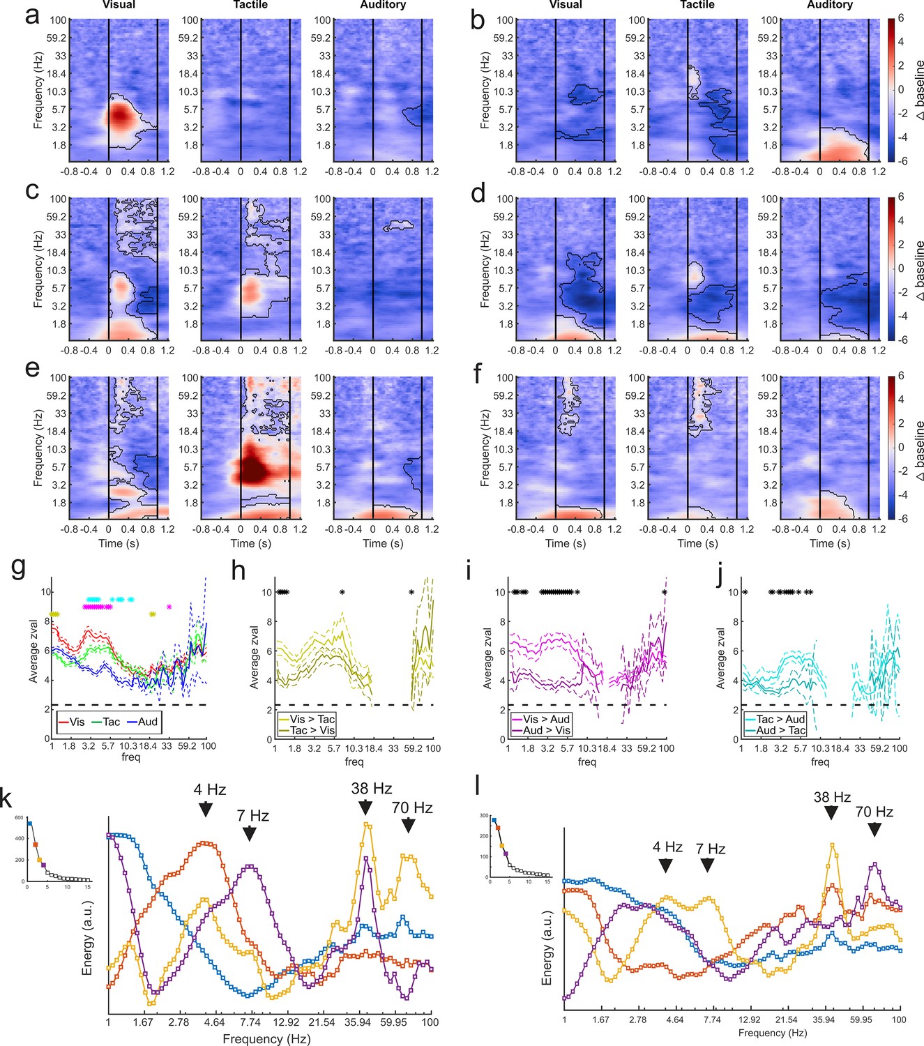
GED-based components show modality-selective but not modality-specific changes in multiple frequency bands.

(**a–f**) Example time-frequency plots created from the GED-based components separated by stimulus modality (i.e., visual, tactile, and auditory). Each time-frequency plot shows the relative difference in power between the baseline and stimulus periods for a GED-based component time series (scale at far right, 1–100 Hz, logarithmic scale). Black contoured lines denote clusters of significant changes in power between baseline and stimulus delivery (see Materials and methods). Solid lines at 0 and 1 s denote the start and end of stimulus delivery. (a) Increase in power centered around 4.5 Hz elicited by visual stimuli. (b) Increase in power across low (1–3 Hz) frequencies elicited by auditory stimuli with minor power changes for visual and tactile stimuli. (c) Moderate increase in power from 1 to 2 and 5–8 Hz for visual stimuli and 4–8 Hz for tactile stimuli. (d) Moderate decreases in power for all stimuli, centered around 4 Hz. (e) Disparate responses to visual, tactile, and auditory stimuli. Note how multiple frequencies bands show time varying increases in power for all three stimuli, however, the time-frequency power around 1 Hz is similar between the sensory modalities. (f) A component with fairly similar responses across sensory modalities but note the lack of high frequency activity for auditory stimuli. (g) Maximum separation of the selectivity for sensory modality occurs below 10 Hz. Solid lines represent the mean z-value within significant clusters at each frequency for each modality (visual = red, tactile = green, auditory = blue). Dotted lines denote mean +/- 5 standard errors of the mean. Gold asterisks denote significant differences between the visual and tactile responses, magenta asterisks denote significant differences between visual and auditory, and cyan asterisks denote differences between visual and auditory (Wilcoxon rank-sum tests, p<0.01). (**h–j**) Pairwise comparisons of selectivity between modalities for components that responded to multiple sensory modalities. Solid lines represent mean and dotted lines represent the mean +/- 5 standard errors of mean. Black asterisks denote significant differences (Wilcoxon rank-sum tests, p<0.01). (k) Spectral profiles were generated from the significant components from all sessions. PCA was then used to extract the prominent features of these profiles (right). Corresponding scree plots shown on the left (see Materials and methods). These plots were created using all available data regardless of estimated location of the contact. The spectral profile and scree plots were color coded according to the rank of the associated component (1st = blue; 2nd = orange; 3rd = yellow; 4th = purple). The power at each frequency is plotted in arbitrary units of energy. Arrows highlight peaks in the spectra that correspond to frequencies that have been extensively studied in other brain regions (i.e., delta, theta, and low and high gamma). (l) Same as in (k) but only using data from contacts that were estimated to be within the amygdala. Figure 4—figure supplement 1 shows how removing non-amygdala contacts can – but does not necessarily – impact spectral profiles in two individual recording sessions.

Figure 4—figure supplement 1

Download asset Open asset

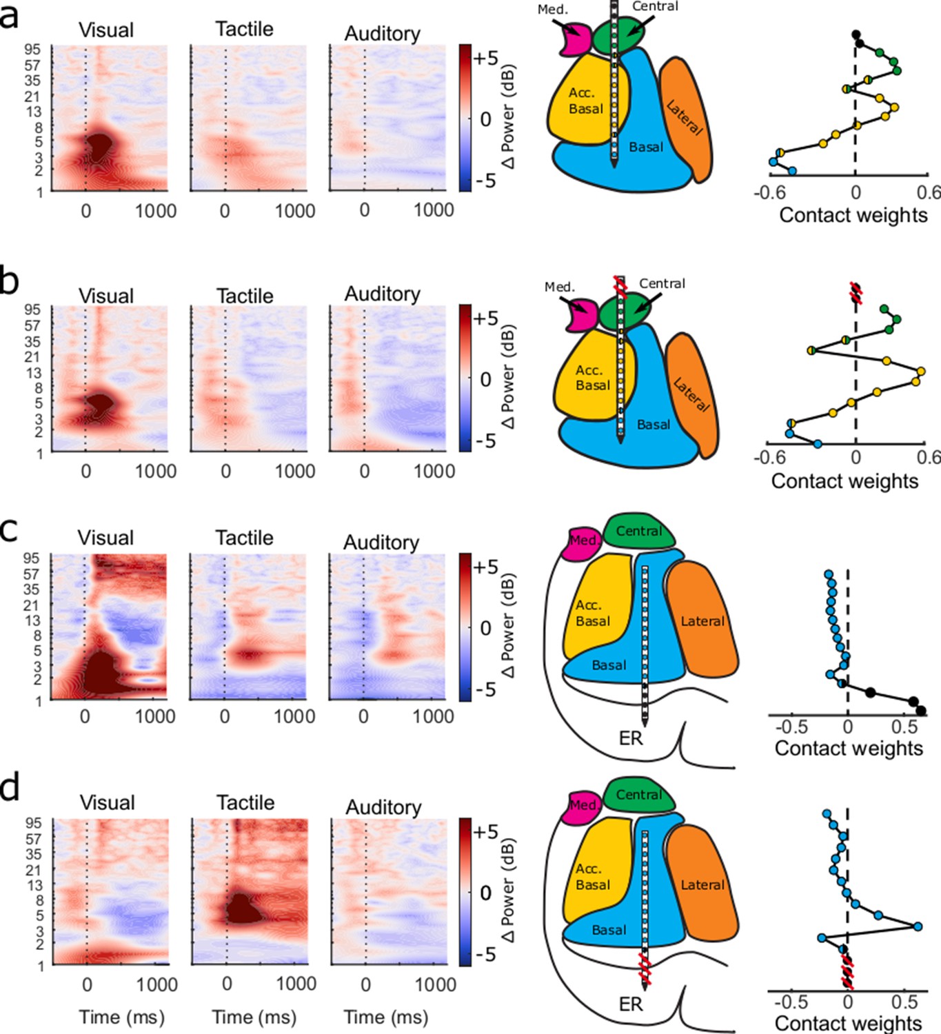
Effects of removing non-amygdala contacts from the GED-based analyses.

The time-frequency plots (left) follow the same convention as in Figure 4, the MRI-based reconstructions (middle) follow the same convention as in Figure 1, and the component map plots (right) follow the same convention as in Figure 2. All results reflect the activity from the component associated with the largest eigenvalue. (a) Results from GED-based analyses from one session generated using LFP collected from all channels regardless of estimated location. (b) Results from the same analyses but when only channels estimated to be located in the amygdala are used (i.e., signal from contacts marked with red lines were not included). Note that there is very little change in the activity of the component (as shown in the time-frequency plots on the left). Likewise, the component map maintains much of its structure, suggesting that activity on the non-amygdala contacts did not influence the component in shown in (a). (c) Results from a different recording session. Note the large changes in power elicited by visual stimuli (particularly between 1–8 Hz and 35+ Hz), the placement of the ventral three contacts in or near the entorhinal cortex, and the component map weights on these central three contacts (relatively large and positive). (d) Results from the same analyses but with the contacts estimated to be ventral to the amygdala removed. Note that the large changes in power in response to visual stimuli are not present in this new component. Instead, large changes in power were elicited by tactile stimuli (mainly between 4–8 Hz). These results demonstrate how removal of non-amygdala contacts can qualitatively have small (**a and b**) or large (**c and d**) impacts on component activity. To assess how these differences manifested across all recordings, we extracted the prominent features of the power spectra across all significant components (Figure 4k and l).

Figure 5

Download asset Open asset

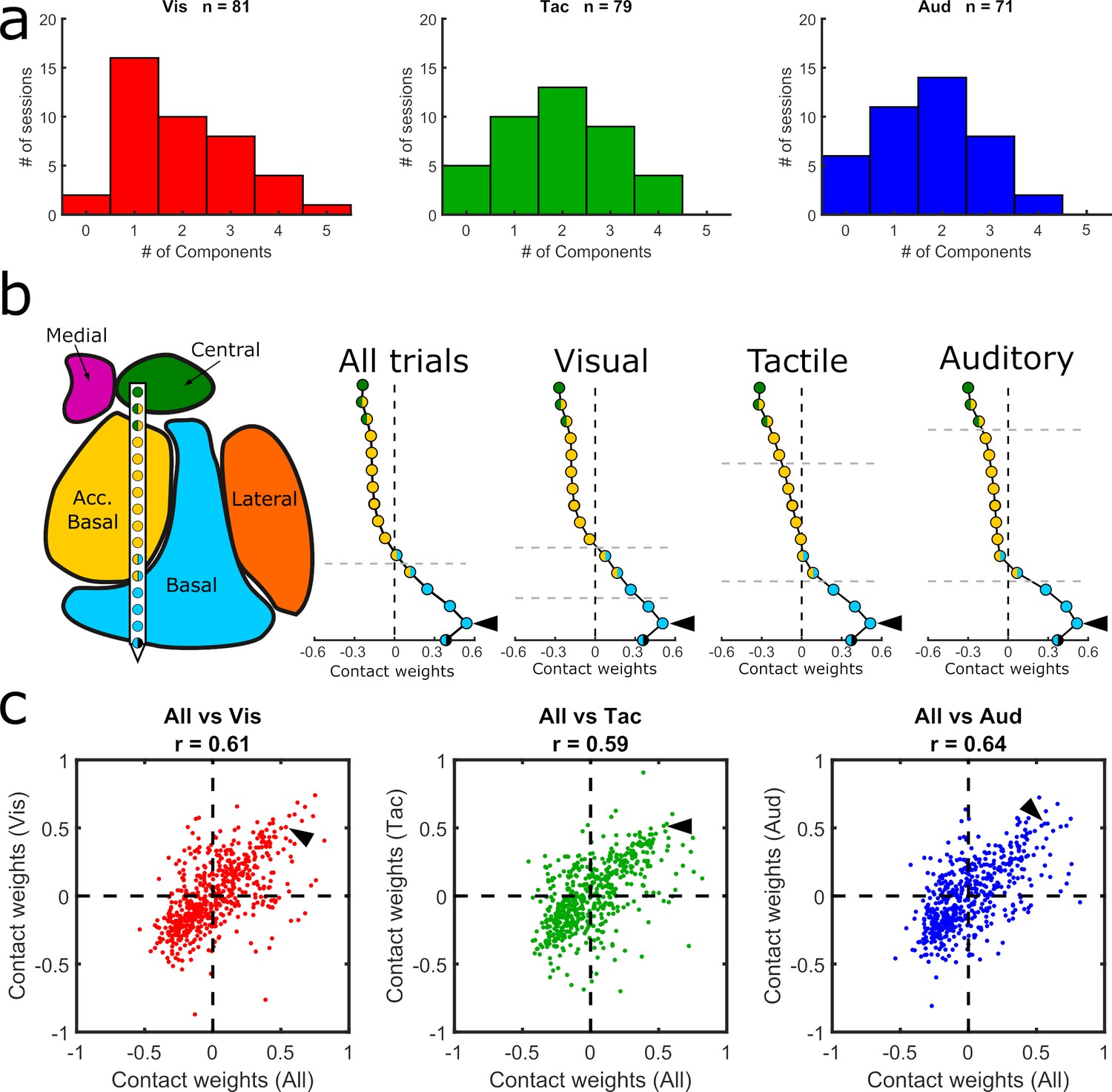
Comparison of GED components across sensory modalities.

(a) Histograms showing the distribution of significant components from visual, tactile, and auditory trials. (b) MRI-based reconstruction of recording sites from an example session (left) and component maps (right) generated from data collected in the same example session using all trials (left) and only visual, tactile, or auditory trials (last three plots in the row). All component maps shown in panel b are based on the first component resulting from each analysis. (c) Pairwise correlations between component maps generated using all trials (x-axis) vs. component maps generated from modality-specific components (y-axis). Each dot shows the paired map projections onto one electrode from one component. Arrowheads in (b) show how the value from a single contact in each of the component maps projected into the scatter plots in (c).

Tables

Table 1

Only visual components significantly map onto anatomical boundaries.

Only the first and second visual component maps matched the anatomical boundaries when correcting for multiple comparisons (paired t-tests, Bonferroni corrected for 12 comparisons, p=0.05/12 = 0.004). C.I. indicates the 95% confidence interval.

	Component #1	Component #2	Component #3	Component #4
Visual	t(38)=3.75 p=0.00059 C.I. = [0.4, 1.56]	t(22)=3.74 p=0.0011 C.I. = [0.57, 1.98]	t(12)=0.25 p=0.81 C.I. = [−0.54, 0.68]	t(4)=−0.054 p=0.62 C.I. = [−1.80, 1.22]
Tactile	t(35)=0.63 p=0.53 C.I. = [−0.34, 0.65]	t(25)=1.97 p=0.06 C.I. = [−0.02, 0.97]	t(12)=1.42 p=0.18 C.I. = [−0.27, 1.29]	t(3)=1.87 p=0.16 C.I. = [−1.03, 3.97]
Auditory	t(34)=−2.46 p=0.019 C.I. = [−0.76,–0.07]	t(23)=−0.74 p=0.47 C.I. = [−0.58, 0.27]	t(9)=−0.02 p=0.99 C.I. = [−0.96, 0.94]	t(1)=−0.97 p=0.51 C.I. = [−14.15, 12.14]