Walking Drosophila navigate complex plumes using stochastic decisions biased by the timing of odor encounters
- Department of Molecular, Cellular and Developmental Biology, Yale University, United States
- Swartz Foundation Fellow, Yale University, United States
- Interdepartmental Neuroscience Program, Yale University, United States
- Department of Physics, Yale University, United States
Figures
Figure 1 with 3 supplements
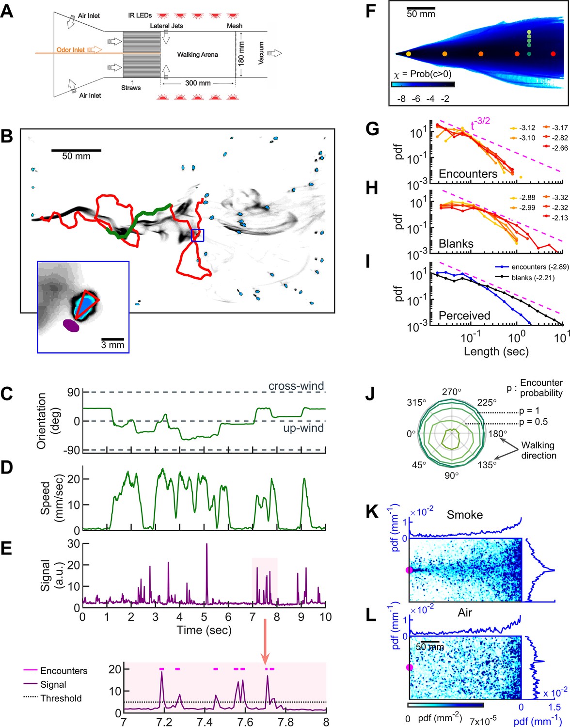
Simultaneous visualization of odor and fly behavior.
(A) Experimental apparatus. The main flow (150 mm/s) is perturbed by lateral jets (1500 mm/s) that alternate stochastically with a characteristic time scale of 100 ms. (B) Walking arena with flies (blue), odor intensity (gray), and a representative trajectory of a navigating fly (red). Green: the portion of the trajectory plotted in C-E. Note that since the odor environment is fluctuating, the image in B only represents the environment at a random time point. Blue rectangle: the area shown in the inset. Inset: blue: fly; gray: odor intensity; red triangle: orientation of the fly; purple: the virtual antenna in which the odor intensity is averaged as a proxy for the signal perceived by the fly. Simultaneous orientation (C), speed (D), and perceived stimulus (E) of the fly while it is navigating in the intermittent plume (green portion of the trajectory in B). Dashed lines in C indicate up-wind and cross-wind orientations. Orientation and speed were smoothed with a 100 ms sliding box filter. The shaded area in E (top) is plotted at a larger scale (bottom) with the sensory threshold (dotted line) used to identify the odor encounters (magenta lines above the signal trace in purple; see also Figure 1—figure supplement 2 and Materials and methods). (F) The fraction of time that odor concentration is above the sensory threshold (i.e. intermittency) at fixed locations. Image intensity is median-filtered (square filter size 2.3 mm), and the likelihood that the intensity is above the sensory threshold, averaged over all frames of the video. Red dots: positions of encounter and blank duration distributions plotted in G-H. Green dots: positions of encounter probability distributions plotted in J. (G-H) Distributions of encounter and blank durations, respectively, at positions color-coded in F. The pink dash line shows the expected from theory for turbulent flow (Celani et al., 2014). Exponents of the power law fit to the tail of the distributions are indicated with the same color code as in F. (I) Odor encounter and blank durations perceived by navigating flies. Values in the parenthesis indicate the exponent of the power law fit to the tail of the distribution. (J) Probability (r axis) to have an odor encounter within 1 s while walking with a speed of 10 mm/s, starting from positions color-coded in F, as a function of walking direction (theta axis). (K) Probability distribution functions (pdf) of fly positions in the arena for the complex smoke plume as in A (n = 1073 trajectories). (L) Same without smoke but with the same complex wind pattern as in K (n = 502). Magenta: location of the source. Blue curves: marginal pdfs.
Figure 1—figure supplement 1
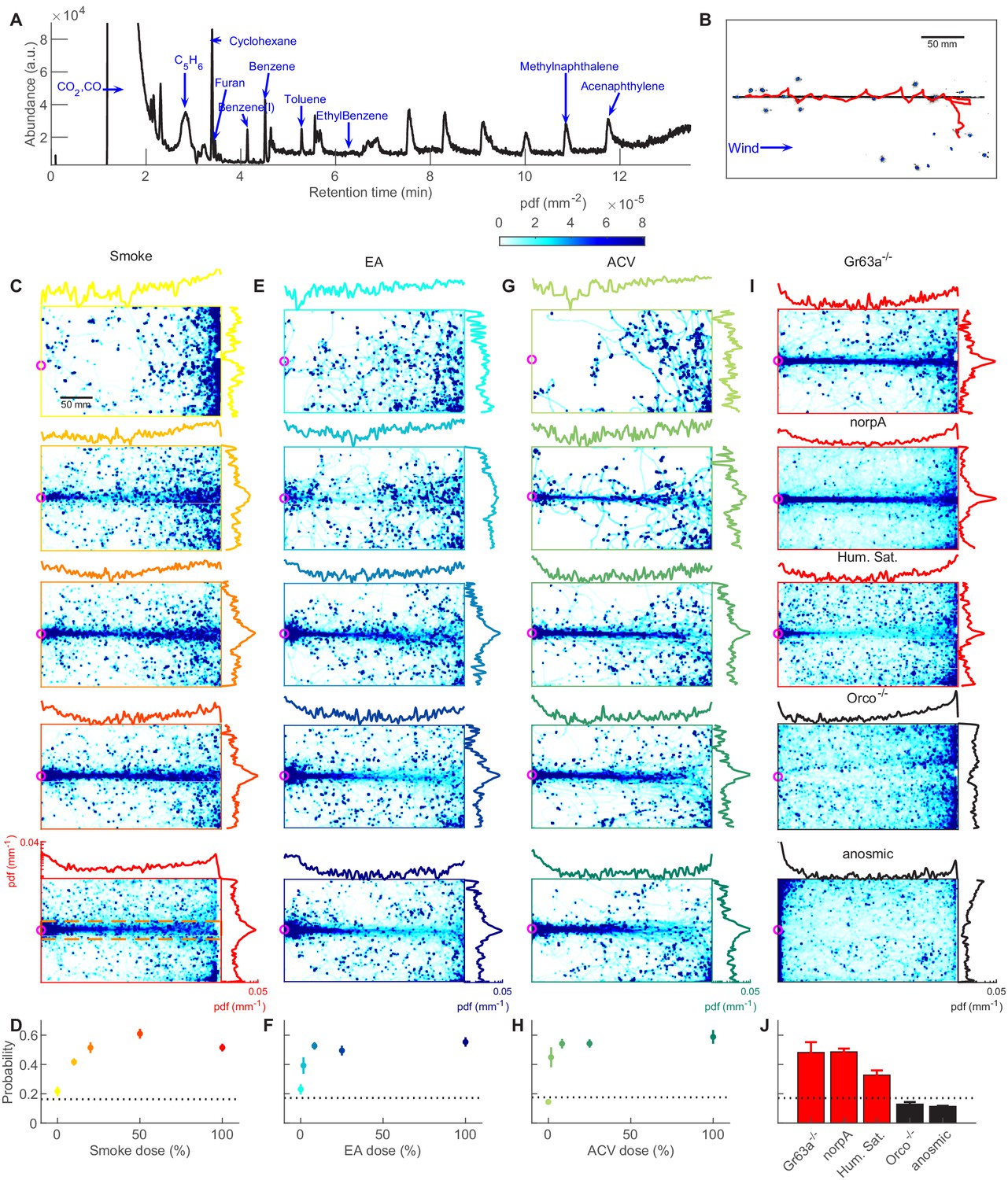
Attraction to smoke is olfactory and dose-dependent, closely mimicking to ethyl acetate and apple cider vinegar.
(A) GC-MS measurement of smoke. Many volatiles belonging to various chemical groups such as alcohols, ketones, and aldehydes are present in the smoke. (B) A snapshot of flies (blue), navigating straight smoke plume (gray) in laminar flow (blue arrow, lateral jets were turned off) with a representative trajectory of a navigating fly (red). (C) Probability distribution functions (pdf) of fly positions in the arena for wild-type CS flies navigating straight plumes (as in B) of smoke with increasing doses (top to bottom, n = 871, 1714, 1600, 1996, 4421 trajectories). Marginal pdfs in the x- or y-direction are plotted on a log scale on the exterior. (D) Integral of pdfs over the ribbon region (orange box, illustrated in the bottom plot of C) as a function of smoke dose. The dashed line represents chance probability. (E–F) Same as C-D but for ethyl acetate (EA, n = 369, 363, 907, 1351, 1604). (G–H) Same as C-D but for apple cider vinegar (ACV, n = 176, 212, 829, 1067, 1332). Dose values reported in C-H are the odor concentration of the straight plume released into the arena from the center straw (3 mm diameter). (I) PDFs in straight smoke plumes (dose 100%) for mutant flies, and at humidity saturation for wild-type CS flies. Mutant flies: Gr63a-/- (n = 1581); norpA (n = 4480); Orco-/- (n = 2420); anosmic (Gr63a-/-, Orco-/-, Ir8a-/-, Ir25a-/-; n = 3992). High humidity: (86.0 ± 3.9%; n = 2772). (J) Pdf integrated over the ribbon region (same region used in F-H) for control experiments.
Figure 1—figure supplement 2
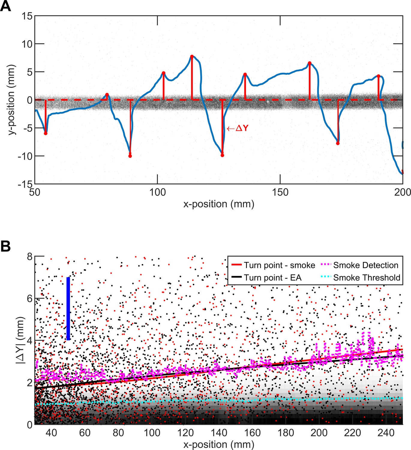
The average turning position of flies in straight plume agrees with smoke intensity.
(A) A representative trajectory of a fly walking around straight smoke plume or ribbon (lateral jets were turned off). Gray: smoke intensity. Blue: the trajectory of the fly. Red dots: points where fly makes a turn toward ribbon. Red line: the distance between ribbon center and turning point (i.e. ΔY). (B) Comparison of smoke diffusivity to turning points of flies in straight plumes of smoke and EA. Red (black) dots: Turning points in straight smoke (EA) plume. Red (black) curves: data smoothed with the lowess method, with the option of resistance to the outliers. Blue bar: Length representing the size of the fly (3 mm) as a guide for the reader. Pink curve: iso-line of smoke intensity at 0.1 (a.u.). Cyan curve: iso-line of smoke intensity at 5 (a.u.) which is the value used for encounter detection.
Figure 1—figure supplement 3
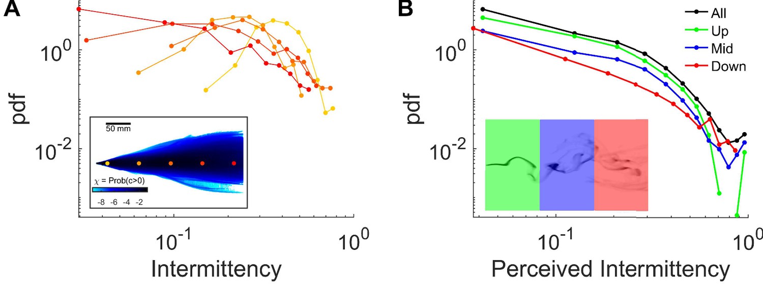
Intermittency in the complex plume.
(A) Distribution of intermittencies at fixed locations, same color codes as in the inset (same as Figure 1F), across the arena in a complex smoke plume. Intermittency is calculated by estimating the fraction of time that smoke intensity is above the sensory threshold over a 2 s sliding window. Inset: (same as Figure 1F) Intermittency at fixed locations: The fraction of time that odor concentration is above the sensory threshold B Intermittency is perceived by flies navigating in a complex plume. Intermittency is calculated as in A using the traces of smoke signal perceived by the flies as they navigated the complex plumes (same data as in Figure 1K). Colors indicate the different regions of the behavioral arena where the flies where located as shown in the inset. Black: all regions, green: between 0 and 100 mm down-wind from the source, blue: between 100 and 200 mm, red: between 200 and 300.
Figure 2 with 1 supplement
Navigation within intermittent complex odor plumes comprises walk-stop transitions and upwind orientation.
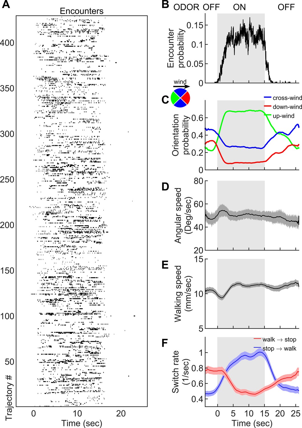
(A) The odor encounters experienced by flies navigating the intermittent smoke plume as in Figure 1B (see also Video 3). While the wind is continuously perturbed by the lateral jets, the odor is turned on/off in 15 s blocks (gray shading). Rows indicate independent trajectories (n = 429) obtained from 267 flies. (B-F) Quantities averaged over all trajectories in A as a function of time. (B) Probability of having an encounter. (C) Probability of being in up-wind (green), cross-wind (blue), and down-wind (red) orientations estimated in 90-degree quadrants as shown in the circle with the same color codes. C-E include only time points for which the fly was walking (v > 2 mm/s). (D) Angular speed. (E) Walking speed. (F) Walk-to-stop (red) and stop-to-walk (blue) switching rates. All quantities in B-F are smoothed with a 5 s sliding box filter. Error bars indicate SEM.
Figure 2—figure supplement 1
Smoke elicits behavior similar to natural odorants.
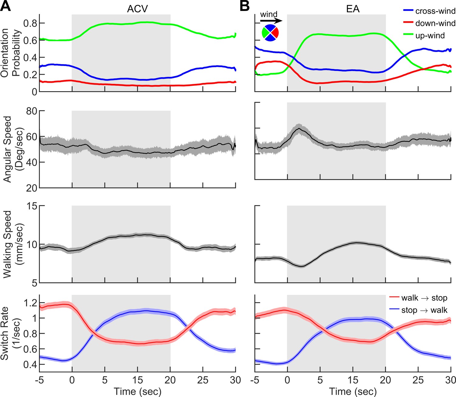
Behavior of flies navigating in the intermittent plumes of A apple cider vinegar (ACV) and B ethyl acetate (EA) as in Figure 2 where the wind is perturbed continuously with random lateral jets whereas the odor is turned on/off over 15 s periods. Quantities averaged over all trajectories in A-B (n = 1830 trajectories for ACV and n = 1809 for EA) as a function of time. 1st row: Probability of being in up-wind (green), cross-wind (blue), and down-wind (red) orientations estimated in 90-degree quadrants as shown in the circle with the same color codes. 2s row: Angular speed, 3rd row: Walking speed, 4th row: Walk-to-stop (red) and stop-to-walk (blue) switching rates. Quantities in all four rows are smoothed with a 5 s sliding box filter. Error bars indicate SEM. Gray area indicates the period that odor injection, into the arena, is turned while the wind is constantly perturbed with lateral jets as in Figure 2.
Figure 3 with 1 supplement
Flies use encounter frequency to bias orientation upwind.
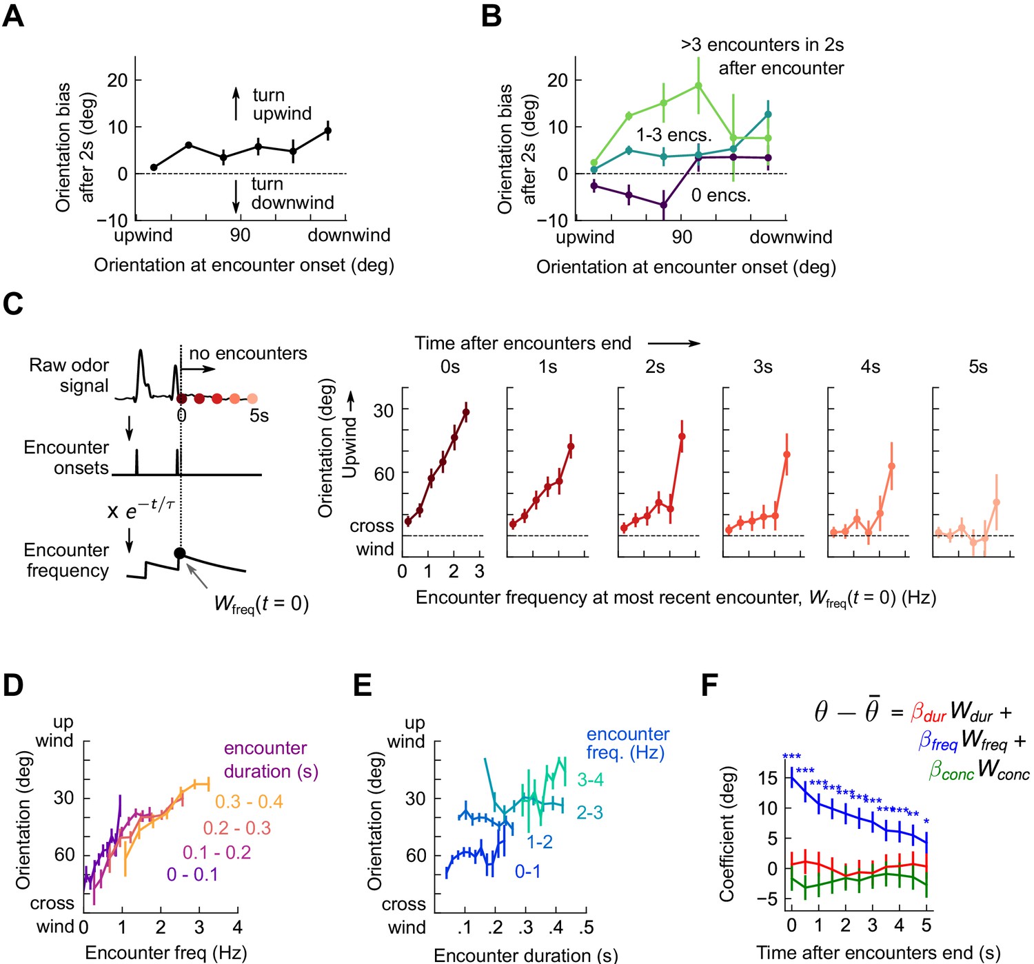
(A) Orientation 2 s after an encounter, as a function of orientation at encounter onset (n=5040). The mean orientation change for random times is subtracted out. (B) Same data, now binned by the number of subsequent encounters in the 2 s window. (C) Orientation as a function of encounter frequency at the most recent encounter, , for various times after encounters have been interrupted. Encounter frequency is defined by convolving the binary vector of encounter onsets with an exponential filter of timescale τ = 2 s. defines the time of the most recent encounter, and the individual plots show fly orientation as a function of the encounter frequency at this time, . Orientation biases strongly upwind with frequency and this correlation vanishes after ~5 s. (D) Orientation versus encounter frequency when encounter duration is held fixed within a small range, for various ranges. (E) Orientation versus encounter duration when encounter frequency held fixed within a small range. (F) Estimated regression coefficients for a trilinear fit of fly orientation to encounter frequency, encounter duration, and signal intensity. Each of the independent variables has been standardized. Coefficients are plotted for various times after encounters are interrupted (as in C). Statistical significances using a 2-tailed t-test are shown next to curves; if no stars are shown, the coefficients are not statistically distinct from 0. The data indicate that orientation correlated with encounter frequency but not encounter duration or signal intensity.
Figure 3—figure supplement 1
Encounter-elicited orientation change in time.
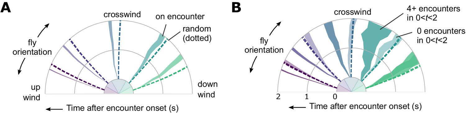
(A) Orientation 2 s window following an encounter (n = 5040), for fly orientations binned in 0–30, 30–60, 60–120, 120–150, and 150–180 degrees, where 0 is upwind and 180 is downwind. Time progresses radially outward. Orientations for random (non-encounter elicited) times are indicated by the dashed lines. (B) Same data, now binned by number of subsequent encounters in the 2 s window.
Figure 4 with 1 supplement
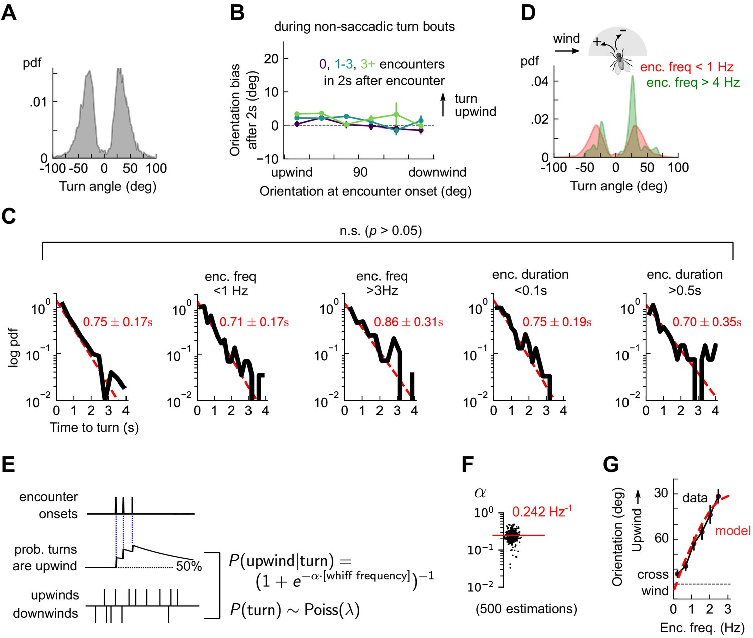
Odor encounters bias turn direction but not turn rate or turn magnitude.
(A) Distribution of change in orientation following a turn. The discreteness of turn angle (two narrow peaks in pdf) was verified to be insensitive to the threshold used to determine turns (Figure 4—figure supplement 1). (B) Cumulative change in orientation over non-turning bouts (‘straight’ segments) 2 s after an encounter, versus orientation at encounter onset (compare with Figure 3B). Data are partitioned into encounters followed by 0, 1-3, or 4+ subsequent encounters in the following 2 s. (C) Leftmost plot: Distribution of time until a turn. Red line: maximum likelihood fit to an exponential distribution, with mean 0.75±0.17 s (distribution generated by bootstrapping). Remaining plots: Same, now for times at which encounter frequency is low (<1Hz; 2nd plot) or high (>3Hz; 3rd plot), or times at which encounter duration is low (<100 ms; 4th plot) or high (>500 ms; 5th plot). Fits are 0.71±0.17 s, 0.86±0.31 s, 0.75±0.19 s, 0.70±0.35 s, respectively, none of which are statistically distinct from the data for all turns (p > 0.05, 2-tailed t-test). (D) Distribution of turn angles during low (< 1 Hz) or high (> 4 Hz) encounter frequency bouts (compare A). (E) Model of fly turning. Turn events obey a Poisson process with timescale τT=0.75s (C). Turn direction is chosen randomly at each turn time, where the probability that the turn is directed upwind is modeled by (Materials and methods). is therefore a sigmoidal function of the frequency of odor encounters , where the gain parameter represents the steepness of the sigmoid. (F) Distribution of gain parameter , estimated for 500 distinct subsets of the data. The distribution is highly peaked, indicating its robustness. The median estimate of is 0.242 Hz−1. (G) Upwind orientation versus encounter frequency for data (black) and model prediction (red).
Figure 4—figure supplement 1
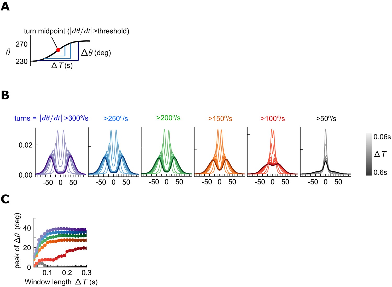
Quantification of turn detection.
(A) Turns occur when the angular speed crosses a threshold. The total change in orientation is the change in angle over some time window centered on the turn time. (B) Distributions of orientation change for various time windows (shades) about the turn midpoint, for various thresholds (colors). For all thresholds > 150 deg/s, orientation change increases with window at first, but then the distributions remain steady, maintaining a bimodal structure. (C) Location of peak for different turn thresholds, as a function of window length . For all thresholds > 150 deg/s, peak remains constant for sufficient .
Figure 5 with 2 supplements
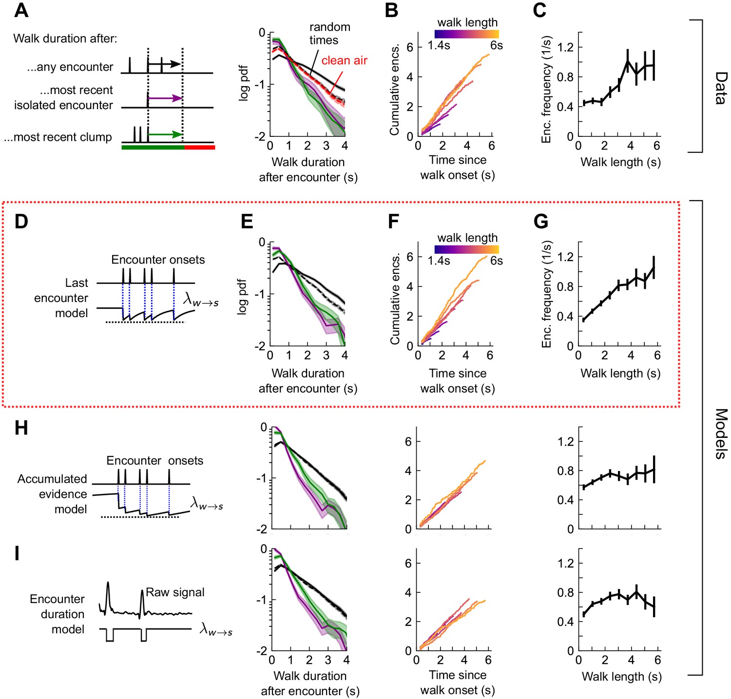
Stop decisions are stochastic events whose rate is modulated by the timing of the most recent encounter.
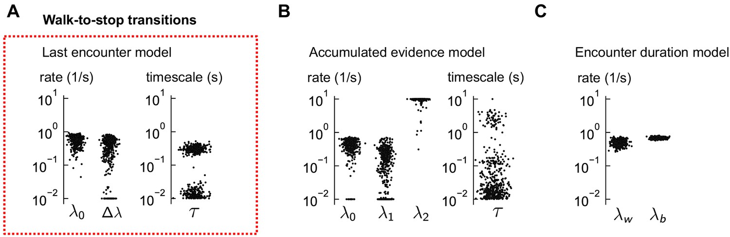
(A) Distribution of walking duration following any odor encounter, or the most recent encounter or clump before a stop. Dashed: distribution for randomly chosen times. Red dashed: clean air control. (B) Cumulative encounter counts since walk onset, for various walk durations. (C) Average encounter frequency versus duration of walk bout. (D) In the last encounter model, stop decisions are modeled as a Poisson process with an inhomogeneous rate , where resets to a fixed value at every encounter, then decays back to baseline. This is modeled by , where is the time since the most recent encounter (Materials and methods for details). Median of estimated parameters are , Δλ=-0.61s-1, τs=0.25s (Figure 5—figure supplement 2). (E-G) Analogs of A-D using data generated by the model. (H) Analogs of E-G for the accumulated evidence model. In this model, decreases at every encounter, but remains at a lower value when encounters are more closely spaced. We model this with . (I) Analogs of E-G for the encounter duration model, in which switches between a low value during encounters and a higher value during blanks.
Figure 5—figure supplement 1
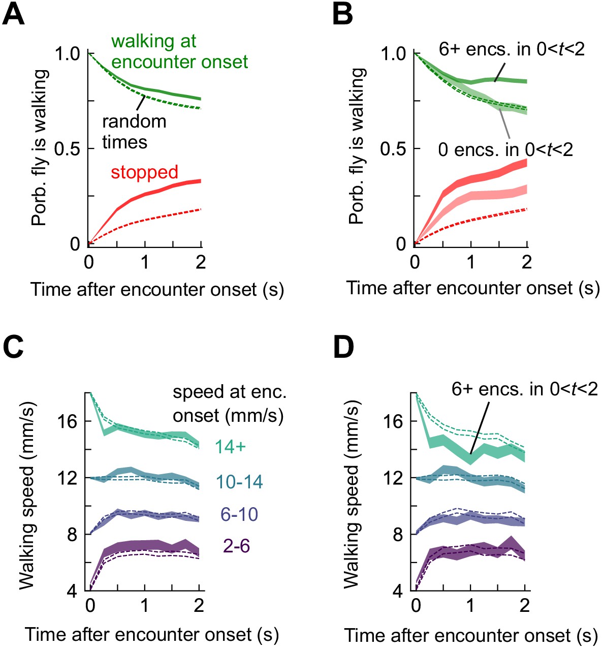
Stop and walk decisions depend on encounter timing.
(A) Probability of walking (green) and being stopped (red) in a 2 s window following an odor encounter (solid) or at random times (dashed). (B) Same, for encounters with zero subsequent encounters (lighter shade) or > 5 subsequent encounters (darker shade) in the following 2 s. (C) Walking speed in a 2 s window following encounters, binned by the speed at encounter onset. Dotted lines indicate randomly chosen times. (D) Same, for six or more subsequent encounters in the 2 s window.
Figure 5—figure supplement 2
Distributions of estimated parameters for walk-to-stop models.
(A) The estimated parameters for the last encounter model of walk-to-stop transitions, using 500 distinct subsets of the data. The red box indicates that this model was the best fit to the data (Figure 5D-G). Occasionally, the global minimum of the nonconvex cost function cannot be found and the optimization terminates near the parameter bounds, rendering the parameter distributions bimodal. (B–C) Same for the other two models, which did not explain the data. In some cases, the minimum consistently lies at the boundary (e.g. in the accumulated evidence model), suggesting that the model is poor. In both models, the predictions were poor (Figure 5H-I).
Figure 6 with 1 supplement
Walk decisions are stochastic events whose rate accumulates evidence from recent encounters.
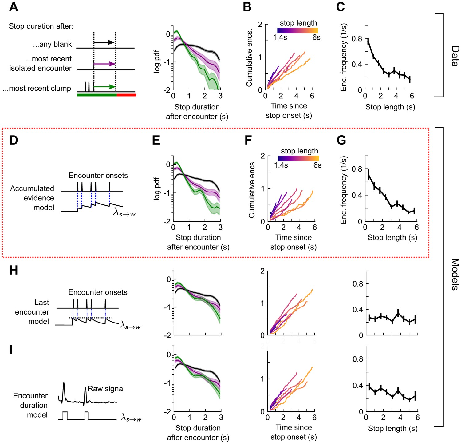
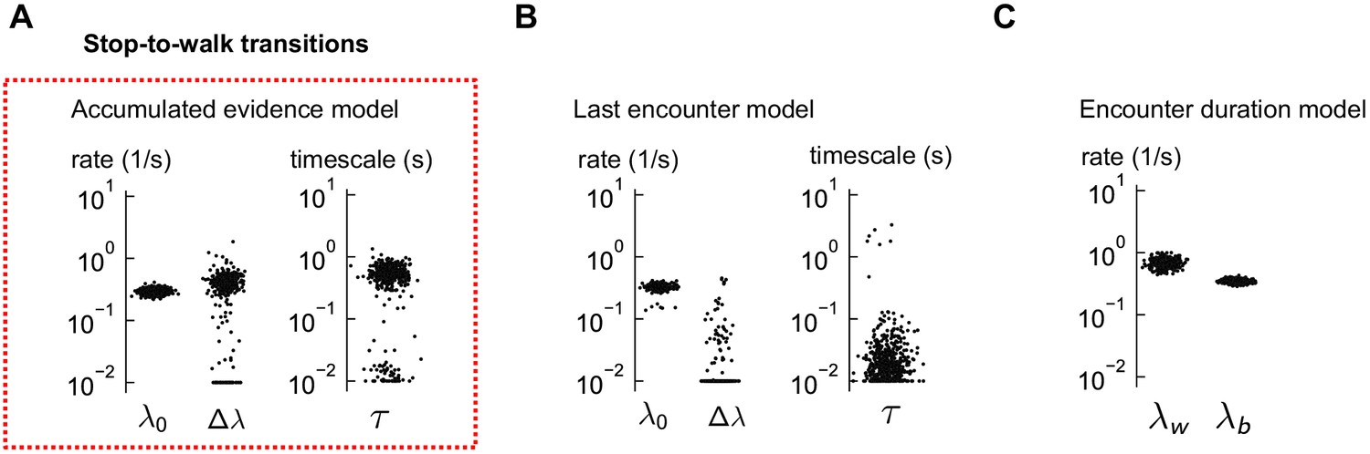
(A) Distribution of stop duration following any encounter, or the most recent encounter or clump before a walk. (B) Cumulative encounter counts since walk onset, for various stop durations. (C) Average encounter frequency versus duration of stop bout. (D) In the accumulated evidence model of walk decisions, increases at every encounter onset, before decaying to baseline. This is modeled by . Median of estimated parameters are λ0=0.29s-1, Δλ=0.41s-1, τw=0.52s (Figure 6—figure supplement 1). (E-G) Analogs of A-C using data generated by the model. (H) Analogs of E-G for the last encounter model, in which the walk rate increases to a fixed value at each encounter before decaying to baseline. (I) Analogs of E-G for the encounter duration model, in which switches between a high value during encounters and low value during blanks.
Figure 6—figure supplement 1
Distributions of estimated parameters for stop-to-walk models.
(A) The estimated parameters for the accumulated evidence model of stop-to-walk transitions, using 500 distinct subsets of the data. (B–C) Same for the other two models, which did not explain the data well. In the last encounter model, the parameter was consistently estimated at its bound (effectively zero). In both models, the predictions were poor (Figure 6H-I).
Figure 7
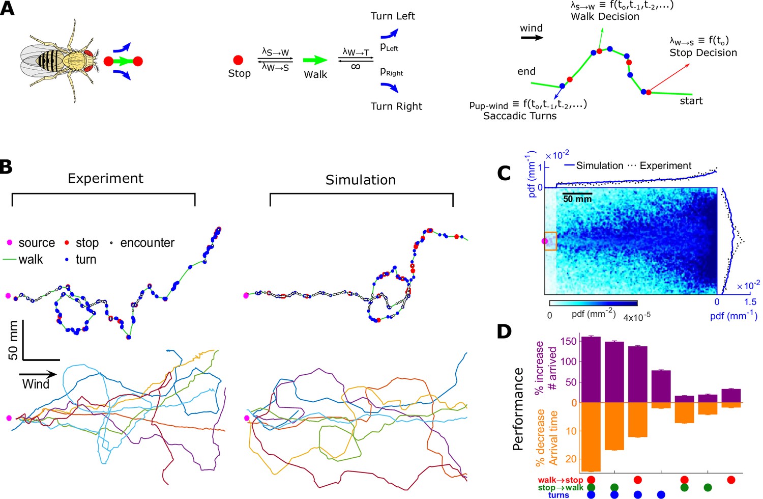
Agent-based simulation reveals navigational performance is significantly improved by encounter-modulated turn and walk decisions.
(A) Agent-based simulation. Left: An agent has four behavioral states: stops, walks, and saccadic turns either left or right. Middle: Diagram of behavioral transitions. Right: Hypothetical trajectory of a virtual fly. Stop-to-walk rates and upwind turn probability depend on encounter history, whereas walk-to-stop rates depend only on the time of the last encounter. (B) Comparison of trajectories of real flies to those of virtual navigators in the complex plume. Top row: Representative trajectories. Bottom row: seven exemplary trajectories that reached within a 15 mm radius of the source. (C) Pdf of virtual flies (n = 10000 trajectories). Magenta: location of the source; blue curves: marginal pdfs over x- and y-direction for the simulation; dotted-black curves: marginal pdfs for the real flies (reproduced from Figure 1K). Very close to the source, the plume becomes ribbon-like, and real flies navigate this region by zigzagging around the slowly meandering ribbon as we have found in static ribbons (Figure 1—figure supplement 1B). In addition, flies tend to aggregate near the front of the arena near the odor inlet once reaching the source region. Since our models describe the navigation strategy in the interior of the plume, rather than this anterior near-source region, we have excluded the front 20 mm of the arena from the marginals. Red rectangle: borders used to determine whether a synthetic navigator reached to the source. (D) Purple: a fractional increase in the number of virtual flies that arrived at the source (borders of red box in C, same width in the y-direction as the one used in our static plumes [Figure 1—figure supplement 1C] and a length of 20 mm in the x-direction), , where NC is the number of control flies that arrived at the source, and Ni is the number of flies arrived at the source for simulation condition i. Simulation conditions i (x-axis) are distinguished by which behavioral components (turn, walk, and stop decisions) were removed. Stop and walk decisions were removed by setting the corresponding transition rate to their averages over all navigators in the full model (left-most bar). Turn decisions were removed by setting the upwind turn probability to its average. Orange: a fractional decrease in the arrival time, , where T is the time to arrive to source. n = 762, 726, 694, 522, 341, 350, 389 trajectories. Error bars represent the SEM calculated by bootstrapping the data 30 times with replacement.
Videos
Video 1
Starved wild-type (CS) female flies navigating in the intermittent smoke plume.
Video 2
Simultaneous quantification of odor stimulus and fly behavior.
Starved wild-type (CS) female flies navigating in the intermittent smoke plume. The trajectory of a single fly (same as in Figure 1A) is displayed with its speed, orientation, and perceived signal. Green and blue dashed lines in the orientation panel represent up-wind and cross-wind orientations, respectively.
Video 3
Starved wild-type (CS) female flies navigating in the intermittent smoke plume.
The smoke valve is turned on/off at 15 s blocks while the wind is kept fluctuating.
Tables
Key resources table
| Reagent type (species) or resource | Designation | Source or reference | Identifiers | Additional information |
|---|---|---|---|---|
| Strain Drosophila melanogaster | Canton-S (CS) | John Carlson | NA | |
| Strain Drosophila melanogaster | Gr63A (w*;+;Gr63A-/-) | Bloomington Drosophila Stock Center | Bloomington: RRID:BDSC_9941 | Jones et al., 2007 |
| Strain Drosophila melanogaster | norpA7 | Bloomington Drosophila Stock Center | Bloomington: RRID:BDSC_5685 | Bloomquist et al., 1988 https://doi.org/10.1016/S0092-8674(88)80017-5(47) |
| Strain Drosophila melanogaster | Orco (w;+;orco[2]) | John Carlson | NA | https://doi.org/10.1038/nature11712 Su et al., 2012 |
| Strain Drosophila melanogaster | Anosmic (Ir8a[1]; Ir25A[2]; Gr63A[1],Orco[1]) | Richard Benton | NA | Ramdya et al., 2015 https://doi.org/10.1038/nature14024 |
| Chemical compound | Ethyl acetate | MilliporeSigma | CAT # 270989 | CAS # 141-78-6 |
| Chemical compound | Apple cider vinegar | Heinz | NA | |
| Software | Matlab, R2018a | MathWorks, Natick, MA | RRID:SCR_001622 | https://www.mathworks.com/products/new_products/release2018a.html |
| Software | Anaconda Distribution | Anaconda Inc, Austin, TX | NA | https://www.anaconda.com/ |
| Software | Python, 3.6.5 | Python Software Foundation | RRID:SCR_008394 | https://www.python.org/downloads/release/python-365/ |
| Other | Fly food | Archon Scientific, Durham, NC | NA | http://archonscientific.com/ |
| Other | Smoke wick | Regin Inc Oxford, CT, USA | S220 | Commercial wick to generate smoke |
Additional files
Download links
A two-part list of links to download the article, or parts of the article, in various formats.
Downloads (link to download the article as PDF)
Open citations (links to open the citations from this article in various online reference manager services)
Cite this article (links to download the citations from this article in formats compatible with various reference manager tools)
Walking Drosophila navigate complex plumes using stochastic decisions biased by the timing of odor encounters
eLife 9:e57524.
https://doi.org/10.7554/eLife.57524


