Tools and Resources

Plant Biology

Accurate and versatile 3D segmentation of plant tissues at cellular resolution

Heidelberg Collaboratory for Image Processing, Heidelberg University, Germany
EMBL, Germany
School of Life Sciences Weihenstephan, Technical University of Munich, Germany
Centre for Organismal Studies, Heidelberg University, Germany
Department of Comparative Development and Genetics, Max Planck Institute for Plant Breeding Research, Germany
School of Life Sciences, University of Warwick, United Kingdom

Jul 29, 2020

https://doi.org/10.7554/eLife.57613

Open access
Copyright information

Figures
Tables
Additional files

14 figures, 11 tables and 4 additional files

Figures

Figure 1

Download asset Open asset

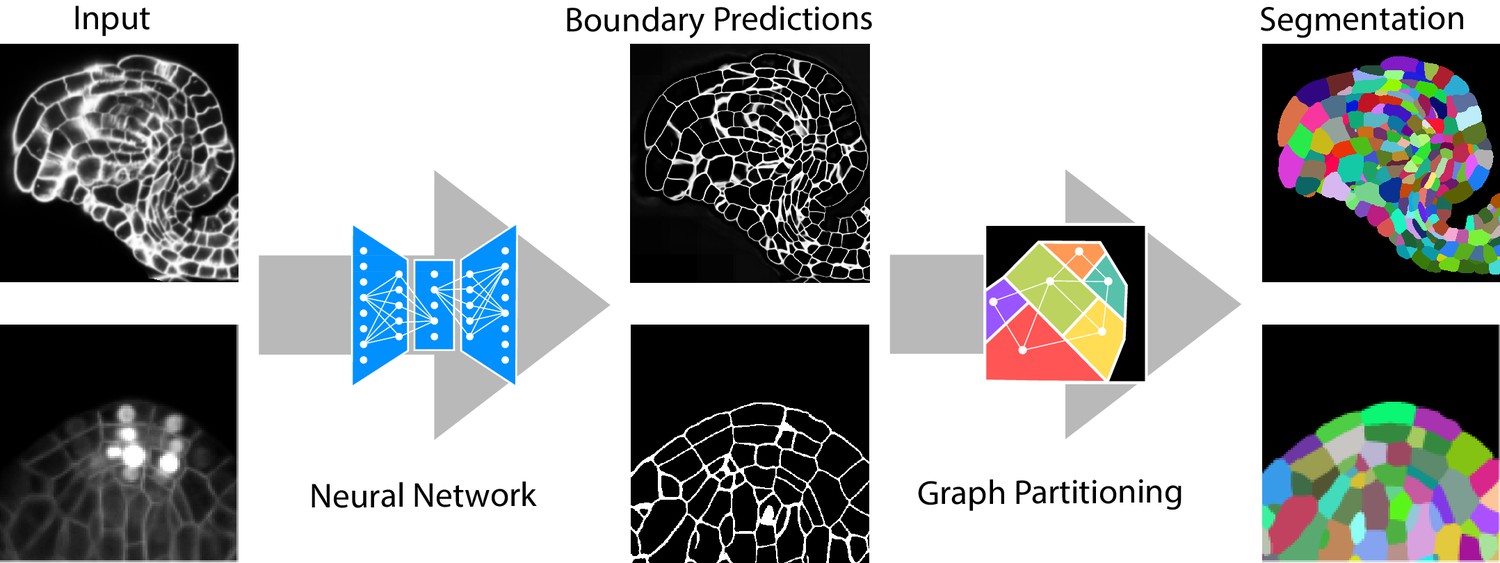
Segmentation of plant tissues into cells using PlantSeg.

First, PlantSeg uses a 3D UNet neural network to predict the boundaries between cells. Second, a volume partitioning algorithm is applied to segment each cell based on the predicted boundaries. The neural networks were trained on ovules (top, confocal laser scanning microscopy) and lateral root primordia (bottom, light sheet microscopy) of *Arabidopsis thaliana*.

Figure 2

Download asset Open asset

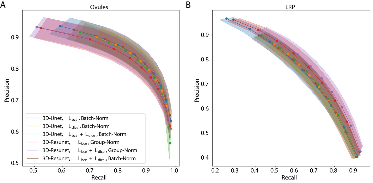
Precision-recall curves for different CNN variants on the ovule (A) and lateral root primordia (LRP) (B) datasets.

Six training procedures that sample different type of architecture (3D U-Net *vs.* 3D Residual U-Net), loss function (BCE *vs.* Dice *vs.* BCE-Dice) and normalization (Group-Norm *vs.* Batch-Norm) are shown. Those variants were chosen based on the accuracy of boundary prediction task: three best performing models on the ovule and three best performing models on the lateral root datasets (see Appendix 5—table 1 for a detailed summary). Points correspond to averages of seven (ovules) and four (LRP) values and the shaded area represent the standard error. For a detailed overview of precision-recall curves on individual stacks we refer to Appendix 4—figure 1. Source files used to generate the plot are available in the Figure 2—source data 1.

Figure 2—source data 1 Source data for precision/recall curves of different CNN variants in Figure 2. The archive contains: 'pmaps_root' - directory containing precision/recall values computed on the test set from the Lateral Root dataset. 'pmaps_ovules' - directory with precision/recall values computed on the test set from the Ovules dataset. 'fig2_precision_recall.ipynb' - Jupyter notebook to generate the plots.: https://cdn.elifesciences.org/articles/57613/elife-57613-fig2-data1-v2.zip
Download elife-57613-fig2-data1-v2.zip

Figure 3

Download asset Open asset

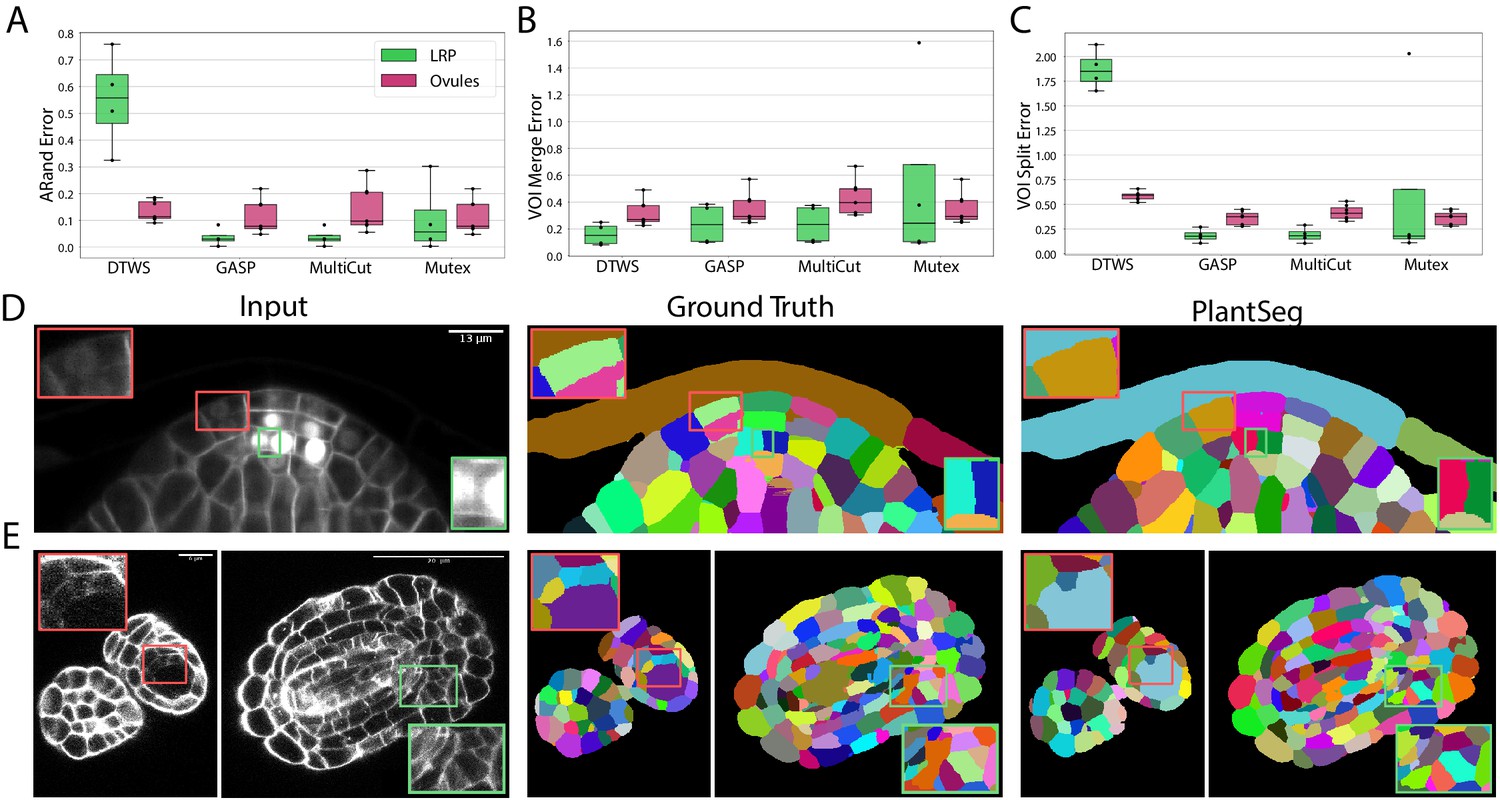
Segmentation using graph partitioning.

(**A–C**) Quantification of segmentation produced by Multicut, GASP, Mutex watershed (Mutex) and DT watershed (DT WS) partitioning strategies. The Adapted Rand error (A) assesses the overall segmentation quality whereas *VOI*_merge (B) and *VOI*_split (C) assess erroneous merge and splitting events (lower is better). Box plots represent the distribution of values for seven (ovule, magenta) and four (LRP, green) samples. (**D, E**) Examples of segmentation obtained with PlantSeg on the lateral root (D) and ovule (E) datasets. Green boxes highlight cases where PlantSeg resolves difficult cases whereas red ones highlight errors. We obtained the boundary predictions using the *generic-confocal-3d-unet* for the ovules dataset and the *generic-lightsheet-3d-unet* for the root. All agglomerations have been performed with default parameters. 3D superpixels instead of 2D superpixels were used. Source files used to create quantitative results shown in (**A–C**) are available in the Figure 3—source data 1.

Figure 3—source data 1 Source data for panes A, B and C in Figure 3. The archive contains CSV files with evaluation metrics computed on the Lateral Root and Ovules test sets. 'root_final_16_03_20_110904.csv' - evaluation metrics for the Lateral Root, 'ovules_final_16_03_20_113546.csv' - evaluation metrics for the Ovules, 'fig3_evaluation_and_supptables.ipynb' - Juputer notebook for generating panes A, B, C in Figure 3 as well as Appendix 5—table 2.: https://cdn.elifesciences.org/articles/57613/elife-57613-fig3-data1-v2.zip
Download elife-57613-fig3-data1-v2.zip

Figure 4

Download asset Open asset

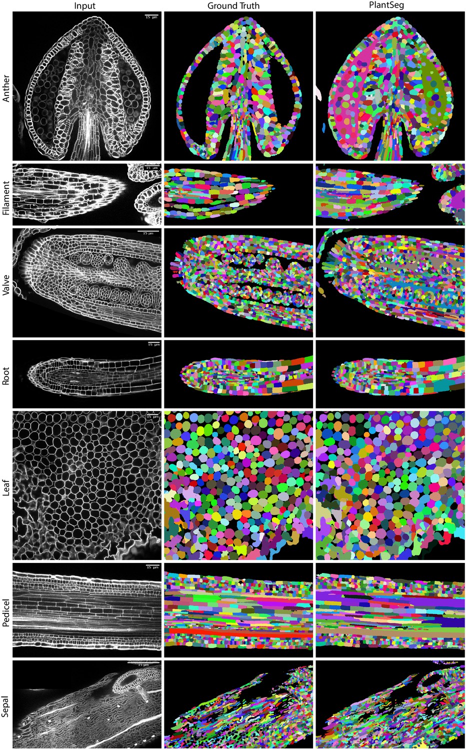
PlantSeg segmentation of different plant organs of the 3D Digital Tissue Atlas dataset, not seen in training.

The input image, ground truth and segmentation results using PlantSeg are presented for each indicated organ.

Figure 5

Download asset Open asset

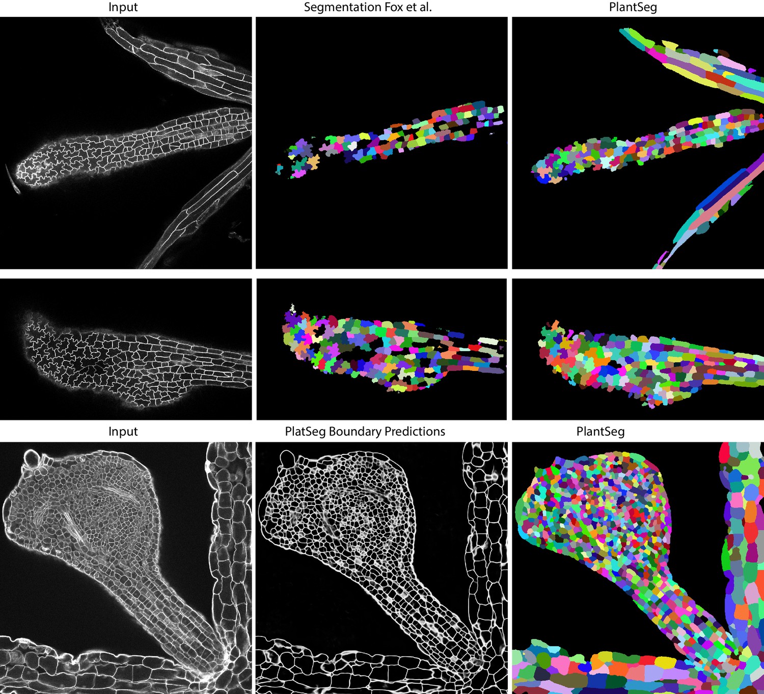
Qualitative results on the highly lobed epidermal cells from Fox et al., 2018.

First two rows show the visual comparison between the SimpleITK (middle) and PlantSeg (right) segmentation on two different image stacks. PlantSeg’s results on another sample is shown in the third row. In order to show pre-trained networks’ ability to generalized to external data, we additionally depict PlantSeg’s boundary predictions (third row, middle). We obtained the boundary predictions using the *generic-confocal-3d-unet* and segmented using GASP with default values. A value of 0.7 was chosen for the under/over segmentation factor.

Figure 6

Download asset Open asset

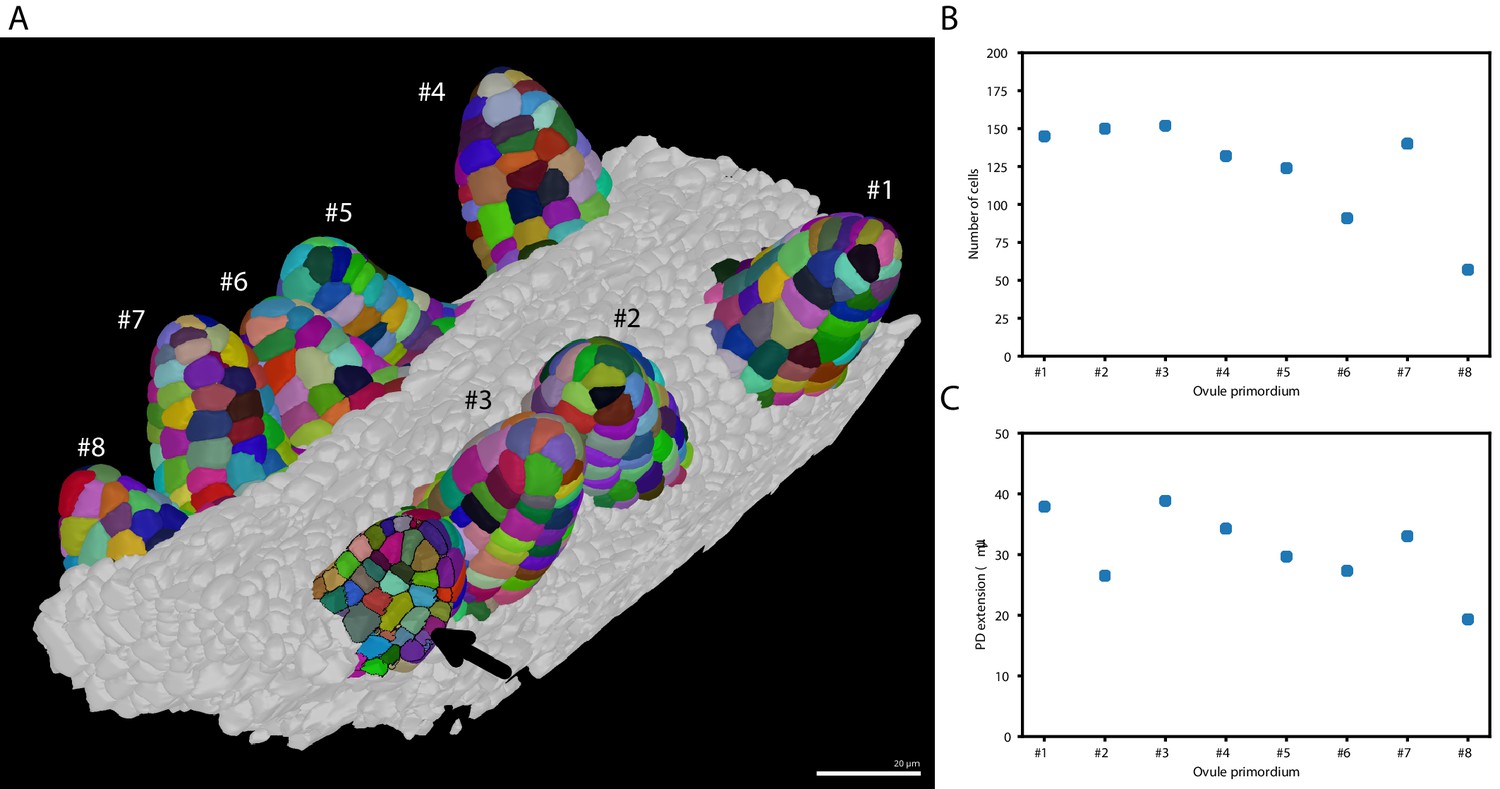
Ovule primordium formation in *Arabidopsis thaliana*.

(A) 3D reconstructions of individually labeled stage 1 primordia of the same pistil are shown (stages according to Schneitz et al., 1995). The arrow indicates an optical mid-section through an unlabeled primordium revealing the internal cellular structure. The raw 3D image data were acquired by confocal laser scanning microscopy according to Tofanelli et al., 2019. Using MorphographX Barbier de Reuille et al., 2015, quantitative analysis was performed on the three-dimensional mesh obtained from the segmented image stack. Cells were manually labeled according to the ovule specimen (from #1 to $# 8$ ). (**B, C**) Quantitative analysis of the ovule primordia shown in (A). (B) shows a graph depicting the total number of cells per primordium. (C) shows a graph depicting the proximal-distal (PD) extension of the individual primordia (distance from the base to the tip). Scale bar: 20 µm. Source files used for creation of the scatter plots (**B, C**) are available in the Figure 6—source data 1.

Figure 6—source data 1 Source data for panes B and C in Figure 6. The archive contains: 'ovule-results.csv' - number of cells and extension for different ovule primordium, 'ovule-scatter.ipynb' - Jupyter notebook for generating panes B and C.: https://cdn.elifesciences.org/articles/57613/elife-57613-fig6-data1-v2.zip
Download elife-57613-fig6-data1-v2.zip

Figure 7

Download asset Open asset

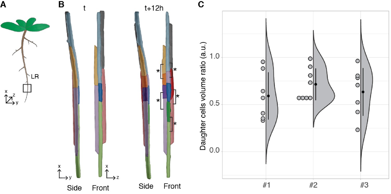
Asymmetric cell division of lateral root founder cells.

(A) Schematic representation of *Arabidopsis thaliana* with lateral roots (LR). The box depicts the region of the main root that initiates LRs. (B) 3D reconstructions of LR founder cells seen from the side and from the front at the beginning of recording (t) and after 12 hr (*t+12*). The star and brackets indicate the two daughter cells resulting from the asymmetric division of a LR founder cell. (C) Half-violin plot of the distribution of the volume ratio between the daughter cells for three different movies (#1, #2 and #3). The average ratio of 0.6 indicates that the cells divided asymmetrically. Source files used for analysis and violin plot creation are available in Figure 7—source data 1.

Figure 7—source data 1 Source data for asymmetric cell division measurements in Figure 7. A detailed description of how to generate the pane C can be found in 'Figure 7C.pdf'.: https://cdn.elifesciences.org/articles/57613/elife-57613-fig7-data1-v2.zip
Download elife-57613-fig7-data1-v2.zip

Figure 8

Download asset Open asset

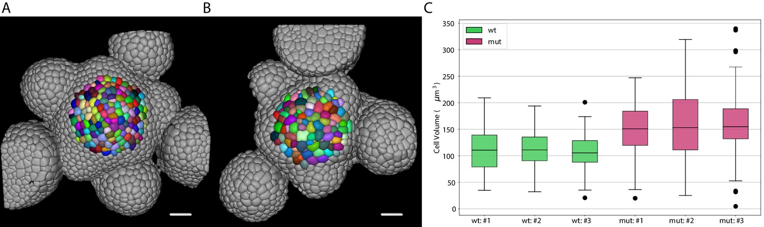
Volume of epidermal cell in the shoot apical meristem of Arabidopsis.

Segmentation of epidermal cells in *wildtype* (A) and *bce* mutant (B). Cells located at the center of the meristem are colored. Scale bar: 20 µm. (C) Quantification of cell volume (µm³) in three different *wildtype* and *bce* mutant specimens. Source files used for cell volume quantification are available in the Figure 8—source data 1.

Figure 8—source data 1 Source data for volume measurements of epidermal cells in the shoot apical meristem (Figure 8). Volume measurements can be found in 'cell_volume_data.csv'. 'fig8_mutant.ipynb' contains the script to generate the plot in pane C.: https://cdn.elifesciences.org/articles/57613/elife-57613-fig8-data1-v2.zip
Download elife-57613-fig8-data1-v2.zip

Figure 9

Download asset Open asset

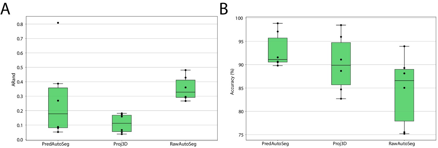
Leaf surface segmentation results.

Reported are the ARand error (A) that assesses the overall segmentation quality and the accuracy (B) measured as percentage of correctly segmented cells (by manual assessment of a trained biologist). For more detailed results, see Appendix 5—table 3.

Figure 9—source data 1 Source data for leaf surface segmentation in Figure 9. The archive contains: 'final_mesh_evaluation - Sheet1.csv' - CSV file with evaluation scores computed on individual meshes, 'Mesh_boxplot.pdf' - detailed steps to reproduce the graphs, 'Mesh_boxplot.ipynb' - python script for generating the graph.: https://cdn.elifesciences.org/articles/57613/elife-57613-fig9-data1-v2.zip
Download elife-57613-fig9-data1-v2.zip

Figure 10

Download asset Open asset

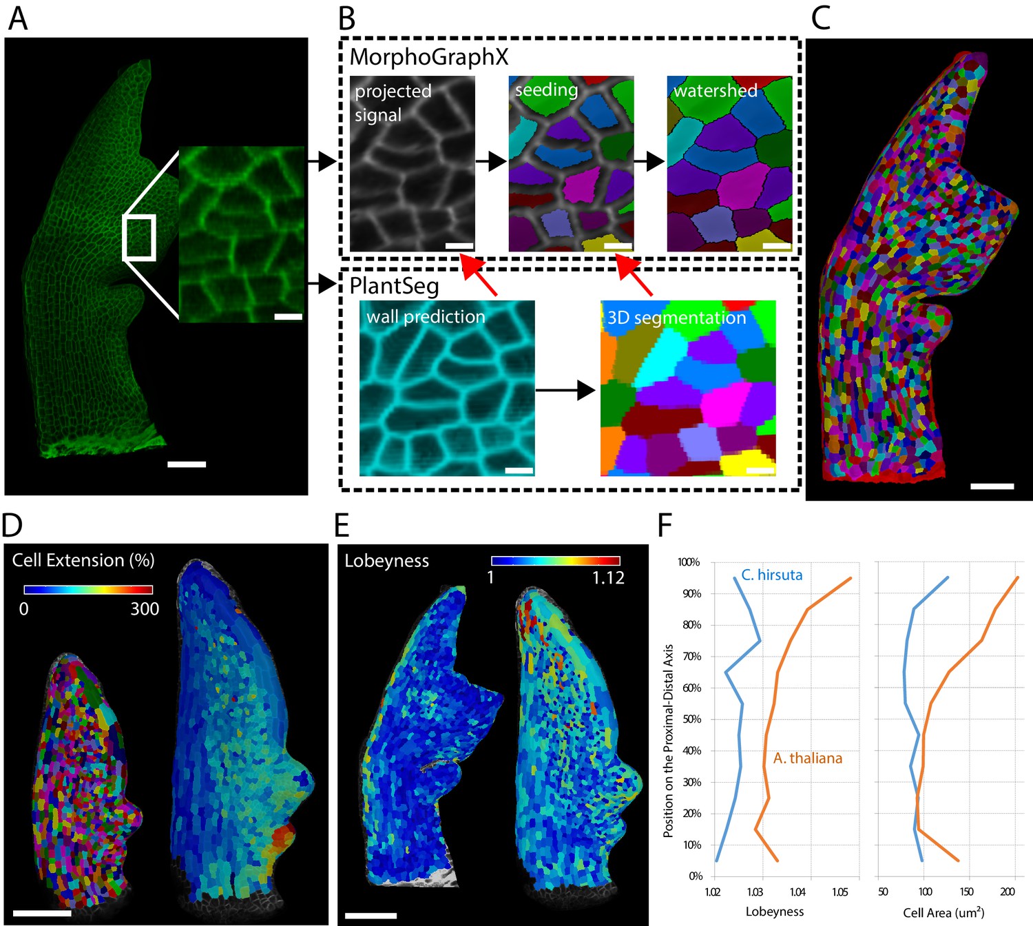
Creation of cellular segmentations of leaf surfaces and downstream quantitative analyses.

(**A–C**) Generation of a surface segmentation of a *C. hirsuta* leaf in MorphoGraphX assisted by PlantSeg. (A) Confocal image of a 5-day-old *C. hirsuta* leaf (leaf number 5) with an enlarged region. (B) Top: Segmentation pipeline of MorphoGraphX: a surface mesh is extracted from the raw confocal data and used as a canvas to project the epidermis signal. A seed is placed in each cell on the surface for watershed segmentation. Bottom: PlantSeg facilitates the segmentation process in two different ways (red arrows): By creating clean wall signals which can be projected onto the mesh instead of the noisy raw data and by projecting the labels of the 3D segmentation onto the surface to obtain accurate seeds for the cells. Both methods reduce segmentation errors with the first method to do so more efficiently. (C) Fully segmented mesh in MorphoGraphX. (**D–F**) Quantification of cell parameters from segmented meshes. (D) Heatmap of cell growth in an *A. thaliana* 8th-leaf 4 to 5 days after emergence. (E) Comparison of cell lobeyness between *A. thaliana* and *C. hirsuta* 600 µm-long leaves. (F) Average cell lobeyness and area in *A. thaliana* and *C. hirsuta* binned by cell position along the leaf proximal-distal axis. Scale bars: 50 µm (**A, C**), 100 µm (**D, E**), 5 µm (inset in A, (B). Source files used for generating quantitative results (**D–F**) are available in Figure 10—source data 1.

Figure 10—source data 1 Source data for pane F in Figure 10 (cell area and lobeyness analysis). 'Figure 10-source data 1.xlsx' contains all the measurements used to generate the plot in pane F.: https://cdn.elifesciences.org/articles/57613/elife-57613-fig10-data1-v2.xlsx
Download elife-57613-fig10-data1-v2.xlsx

Appendix 1—figure 1

Download asset Open asset

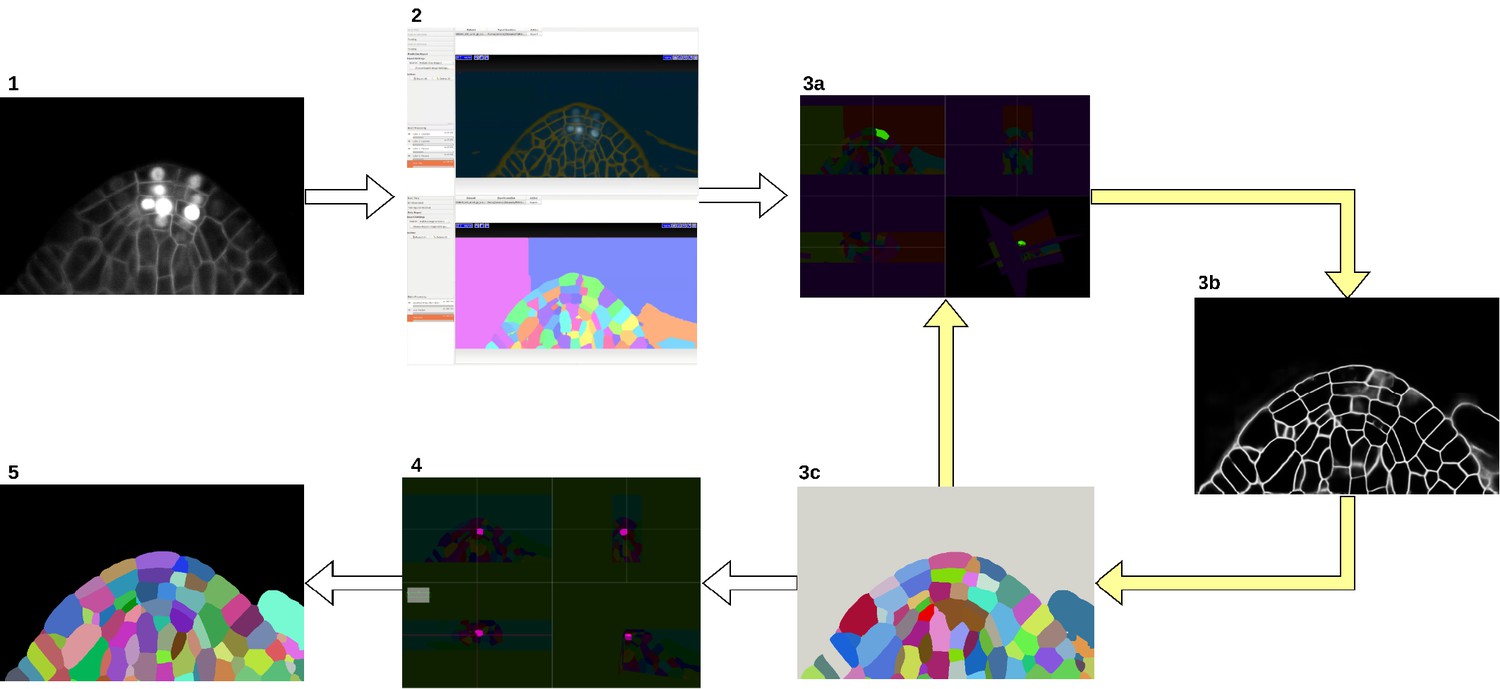
Groundtruth creation process.

Starting from the input image (1), an initial segmentation is obtained using ilastik Autocontext followed by the ilastik multicut workflow (2). Paintera is used to proofread the segmentation (3a) which is used for training a 3D UNet for boundary detection (3b). A graph partitioning algorithm is used to segment the volume (3 c). Steps 3a, 3b and 3 c are iterated until a final round of proofreading with Paintera (4) and the generation of satisfactory final groundtruth labels (5).

Appendix 3—figure 1

Download asset Open asset

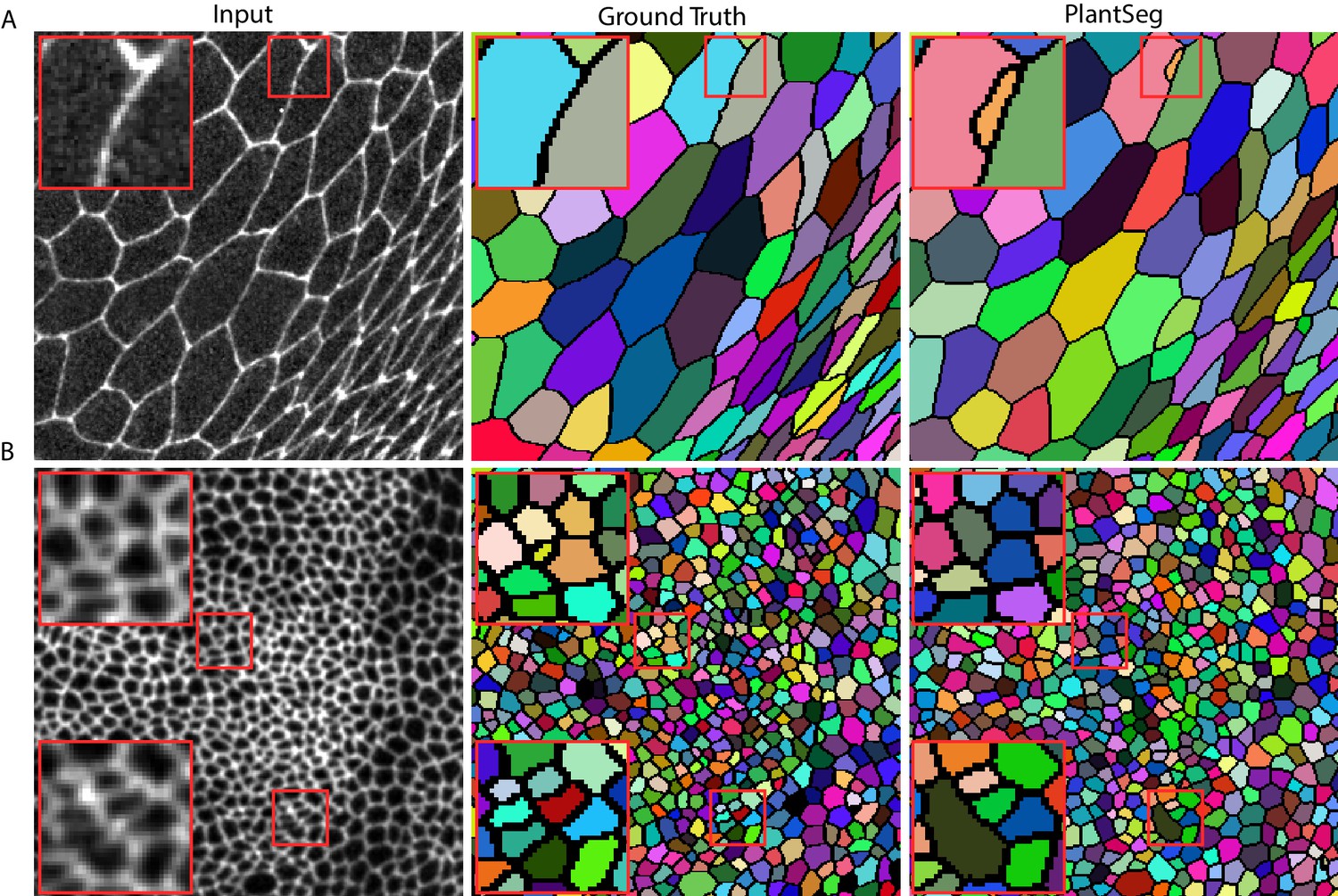
Qualitative results on the Epithelial Cell Benchmark.

From top to bottom: Peripodial cells (A), Proper disc cells (B). From left to right: raw data, groundtruth segmentation, PlantSeg segmentation results. PlantSeg provides accurate segmentation of both tissue types using only the networks pre-trained on the *Arabidopsis* ovules dataset. Red rectangles show sample over-segmentation (A) and under-segmentation (B) errors. Boundaries between segmented regions are introduced for clarity and they are not present in the pipeline output.

Appendix 4—figure 1

Download asset Open asset

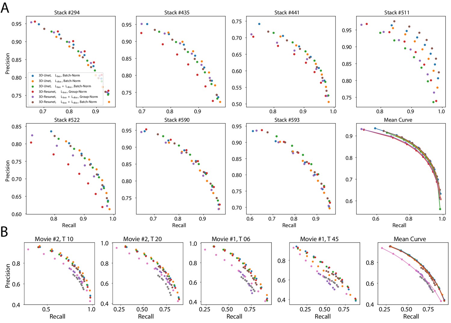
Precision-recall curves on individual stacks for different CNN variants on the ovule (A) and lateral root primordia (B) datasets.

Efficiency of boundary prediction was assessed for seven training procedures that sample different type of architecture (3D U-Net *vs.* 3D Residual U-Net), loss function (BCE *vs.* Dice *vs.* BCE-Dice)) and normalization (Group-Norm (GN) *vs.* Batch-Norm (BN)). The larger the area under the curve, the better the precision. Source files used to generate the precision-recall curves are available in the Appendix 4—figure 1—source data 1.

Appendix 4—figure 1—source data 1 Source data for precision/recall curves of different CNN variants evaluated on individual stacks. 'pmaps_root' contains precision/recall values computed on the test set from the Lateral Root dataset, 'pmaps_ovules' contains precision/recall values computed on the test set from the Ovules dataset, 'fig2_precision_recall.ipynb' is a Jupyter notebook generating the plots.: https://cdn.elifesciences.org/articles/57613/elife-57613-app4-fig1-data1-v2.zip
Download elife-57613-app4-fig1-data1-v2.zip

Appendix 6—figure 1

Download asset Open asset

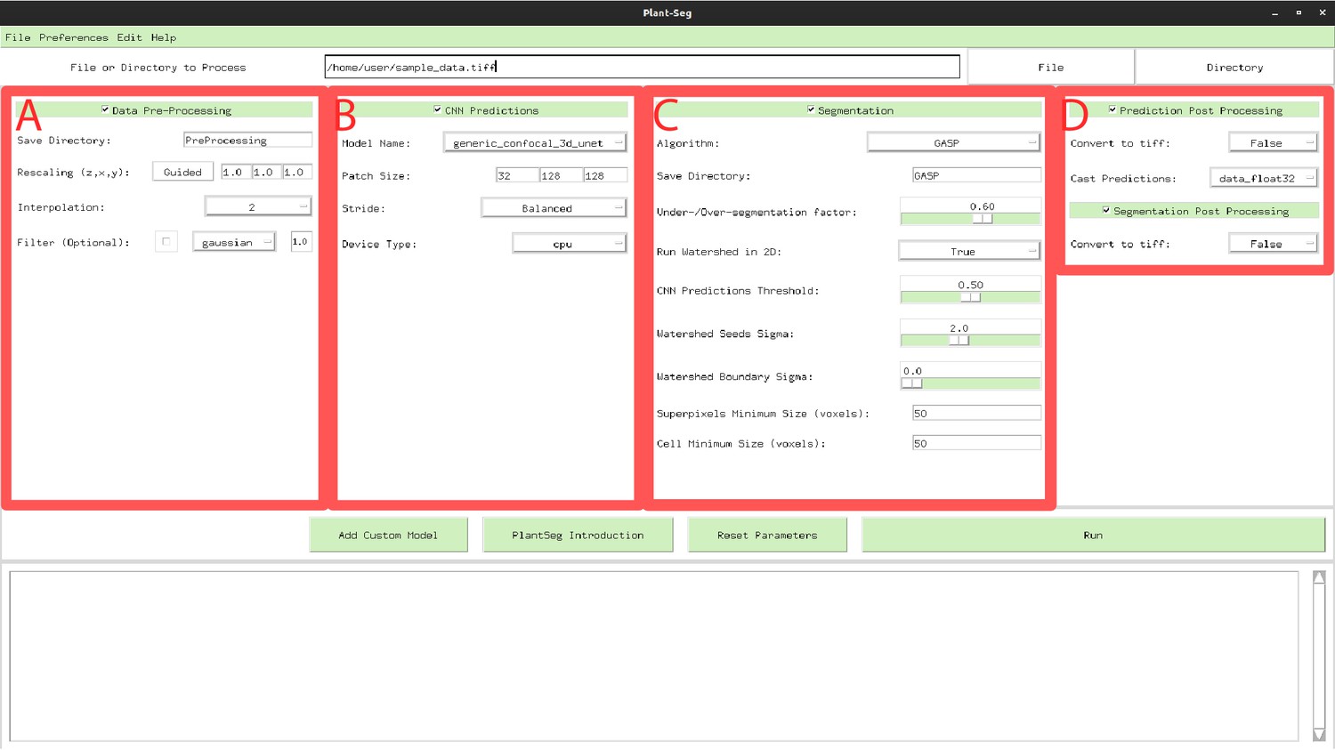
PlantSeg GUI.

The interface allows to configure all execution steps of the segmentation pipeline, such as: selecting the neural network model and specifying hyperparameters of the partitioning algorithm. Appendix 6—table 1 describes the Pre-processing (A) parameters. Appendix 6—table 2 provides parameters guide for the CNN Predictions and Post-processing (**B, D**). Hyperparameters for Segmentation and Post-processing (**C, D**) are described in Appendix 6—table 3.

Tables

Table 1

Quantification of PlantSeg performance on the 3D Digital Tissue Atlas, using PlantSeg .

The Adapted Rand error (ARand) assesses the overall segmentation quality whereas VOI_merge and VOI_split assess erroneous merge and splitting events. The petal images were not included in our analysis as they are very similar to the leaf and the ground truth is fragmented, making it difficult to evaluate the results from the pipeline in a reproducible way. Segmented images are computed using GASP partitioning with default parameters (left table) and fine-tuned parameters described in Appendix 7: Empirical Example of parameter tuning (right table).

Dataset	PlantSeg (default parameters)			PlantSeg (tuned parameters)
Dataset	ARand	VOI_split	VOI_merge	ARand	VOI_split	VOI_merge
Anther	0.328	0.778	0.688	0.167	0.787	0.399
Filament	0.576	1.001	1.378	0.171	0.687	0.487
Leaf	0.075	0.353	0.322	0.080	0.308	0.220
Pedicel	0.400	0.787	0.869	0.314	0.845	0.604
Root	0.248	0.634	0.882	0.101	0.356	0.412
Sepal	0.527	0.746	1.032	0.257	0.690	0.966
Valve	0.572	0.821	1.315	0.300	0.494	0.875

Appendix 3—table 1

Epithelial Cell Benchmark results.

We compare PlantSeg to four other methods using the standard SEG metric (Maška et al., 2014) calculated as the mean of the Jaccard indices between the reference and the segmented cells in a given movie (higher is better). Mean and standard deviation of the SEG score are reported for peripodial (three movies) and proper disc (five movies) cells. Additionally we report the scores of PlantSeg pipeline executed with a network trained explicitly on the epithelial cell dataset (last row).

Method	Peripodial	Proper disc
MALA	0.907 0.029	0.817 0.009
FFN	0.879 0.035	0.796 0.013
MLT-GLA	0.904 0.026	0.818 0.010
TA	-	0.758 0.009
PlantSeg	0.787 0.063	0.761 0.035
PlantSeg (trained)	0.885 0.056	0.800 0.015

Appendix 5—table 1

Ablation study of boundary detection accuracy.

Accuracy of boundary prediction was assessed for twelve training procedures that sample different type of architecture (3D U-Net vs. 3D Residual U-Net), loss function (BCE vs. Dice vs. BCE-Dice) and normalization (Group-Norm vs. Batch-Norm). All entries are evaluated at a fix threshold of 0.5. Reported values are the means and standard deviations for a set of seven specimen for the ovules and four for the lateral root primordia. Source files used to create the table are available in the Appendix 5—table 1—source data 1.

Network and resolution	Accuracy (%)	Precision	Recall	F 1
Ovules
3D-Unet, L_bce, Group-Norm	97.9 1.0	0.812 0.083	0.884 0.029	0.843 0.044
3D-Unet, L_bce, Batch-Norm	98.0 1.1	0.815 0.084	0.892 0.035	0.849 0.047
3D-Unet, L_dice, Group-Norm	97.6 1.0	0.765 0.104	0.905 0.023	0.824 0.063
3D-Unet, L_dice, Batch-Norm	97.8 1.1	0.794 0.084	0.908 0.030	0.844 0.048
3D-Unet, $L_{b c e} + L_{d i c e}$ , Group-Norm	97.8 1.1	0.793 0.086	0.907 0.026	0.843 0.048
3D-Unet, $L_{b c e} + L_{d i c e}$ , Batch-Norm	97.9 0.9	0.800 0.081	0.898 0.025	0.843 0.041
3D-Resunet, L_bce, Group-Norm	97.9 0.9	0.803 0.090	0.880 0.021	0.837 0.050
3D-Resunet, L_bce, Batch-Norm	97.9 1.0	0.811 0.081	0.881 0.031	0.841 0.042
3D-Resunet, L_dice, Group-Norm	95.9 2.6	0.652 0.197	0.889 0.016	0.730 0.169
3D-Resunet, L_dice, Batch-Norm	97.9 1.1	0.804 0.087	0.894 0.035	0.844 0.051
3D-Resunet, $L_{b c e} + L_{d i c e}$ , Group-Norm	97.8 1.1	0.812 0.085	0.875 0.026	0.839 0.044
3D-Resunet, $L_{b c e} + L_{d i c e}$ , Batch-Norm	98.0 1.0	0.815 0.087	0.892 0.035	0.848 0.050
Lateral Root Primordia
3D-Unet, L_bce, Group-Norm	97.1 1.0	0.731 0.027	0.648 0.105	0.684 0.070
3D-Unet, L_bce, Batch-Norm	97.2 1.0	0.756 0.029	0.637 0.114	0.688 0.080
3D-Unet, L_dice, Group-Norm	96.1 1.1	0.587 0.116	0.729 0.094	0.644 0.098
3D-Unet, L_dice, Batch-Norm	97.0 0.9	0.685 0.013	0.722 0.103	0.700 0.056
3D-Unet, $L_{b c e} + L_{d i c e}$ , Group-Norm	96.9 1.0	0.682 0.029	0.718 0.095	0.698 0.060
3D-Unet, $L_{b c e} + L_{d i c e}$ , Batch-Norm	97.0 0.8	0.696 0.012	0.716 0.101	0.703 0.055
3D-Resunet, L_bce, Group-Norm	97.3 1.0	0.766 0.039	0.668 0.089	0.712 0.066
3D-Resunet, L_bce, Batch-Norm	97.0 1.1	0.751 0.042	0.615 0.116	0.673 0.086
3D-Resunet, L_dice, Group-Norm	96.5 0.9	0.624 0.095	0.743 0.092	0.674 0.083
3D-Resunet, L_dice, Batch-Norm	97.0 0.9	0.694 0.019	0.724 0.098	0.706 0.055
3D-Resunet, $L_{b c e} + L_{d i c e}$ , Group-Norm	97.2 1.0	0.721 0.048	0.735 0.076	0.727 0.059
3D-Resunet, $L_{b c e} + L_{d i c e}$ , Batch-Norm	97.0 0.9	0.702 0.024	0.703 0.105	0.700 0.063

Appendix 5—table 1—source data 1 Source data for the ablation study of boundary detection accuracy in Source data for the average segmentation accuracy of different segmentation algorithms in Appendix 5—table 1. 'pmaps_root' contains evaluation metrics computed on the test set from the Lateral Root dataset, 'pmaps_ovules' contains evaluation metrics computed on the test set from the Ovules dataset, 'fig2_precision_recall.ipynb' is a Jupyter notebook generating the plots.: https://cdn.elifesciences.org/articles/57613/elife-57613-app5-table1-data1-v2.zip
Download elife-57613-app5-table1-data1-v2.zip

Appendix 5—table 2

Average segmentation accuracy for different segmentation algorithms.

The average is computed from a set of seven specimen for the ovules and four for the lateral root primordia (LRP), while the error is measured by standard deviation. The segmentation is produced by multicut, GASP, mutex watershed (Mutex) and DT watershed (DTWS) clustering strategies. We additionally report the scores given by the lifted multicut on the LRP dataset. The Metrics used are the Adapted Rand error to asses the overall segmentation quality, the VOI_merge and VOI_split respectively assessing erroneous merge and splitting events (lower is better for all metrics). Source files used to create the table are available in the Appendix 5—table 2—source data 1.

Segmentation	ARand	VOI_split	VOI_merge
Ovules
DTWS	0.135 0.036	0.585 0.042	0.320 0.089
GASP	0.114 0.059	0.357 0.066	0.354 0.109
MultiCut	0.145 0.080	0.418 0.069	0.429 0.124
Mutex	0.115 0.059	0.359 0.066	0.354 0.108
Lateral Root Primordia
DTWS	0.550 0.158	1.869 0.174	0.159 0.073
GASP	0.037 0.029	0.183 0.059	0.237 0.133
MultiCut	0.037 0.029	0.190 0.067	0.236 0.128
Lifted Multicut	0.040 0.039	0.162 0.068	0.287 0.207
Mutex	0.105 0.118	0.624 0.812	0.542 0.614

Appendix 5—table 2—source data 1 Source data for the average segmentation accuracy of different segmentation algorithms in Appendix 5—table 2. The archive contains CSV files with evaluation metrics computed on the Lateral Root and Ovules test sets. 'root_final_16_03_20_110904.csv' - evaluation metrics for the Lateral Root, 'ovules_final_16_03_20_113546.csv' - evaluation metrics for the Ovules.: https://cdn.elifesciences.org/articles/57613/elife-57613-app5-table2-data1-v2.zip
Download elife-57613-app5-table2-data1-v2.zip

Appendix 5—table 3

Average segmentation accuracy on leaf surfaces.

The evaluation was computed on six specimen (data available under: https://osf.io/kfx3d) with the segmentation methodology presented in section Analysis of leaf growth and differentiation. The Metrics used are: the ARand error to asses the overall segmentation quality, the VOI_merge and VOI_split assessing erroneous merge and splitting events respectively, and accuracy (Accu.) measured as percentage of correctly segmented cells (lower is better for all metrics except accuracy). For the Proj3D method a limited number of cells (1.04% mean across samples) was missing due to segmentation errors and required manual seeding. While it is not possible to quantify the favorable impact on the ARand and VOIs scores, we can assert that the Proj3D accuracy has been overestimated by approximately 1.04%.

Segmentation	ARand	VOI_split	VOI_merge	Accu. (%)	ARand	VOI_split	VOI_merge	Accu. (%)
	Sample 1 (Arabidopsis, Col0_07 T1)				Sample 2 (Arabidopsis, Col0_07 T2)
PredAutoSeg	0.387	0.195	0.385	91.561	0.269	0.171	0.388	89.798
Proj3D	0.159	0.076	0.273	82.700	0.171	0.078	0.279	84.697
RawAutoSeg	0.481	0.056	0.682	75.527	0.290	0.064	0.471	75.198
	Sample 3 (Arabidopsis, Col0_03 T1)				Sample 4 (Arabidopsis, Col0_03 T2)
PredAutoSeg	0.079	0.132	0.162	90.651	0.809	0.284	0.944	90.520
Proj3D	0.065	0.156	0.138	88.655	0.181	0.228	0.406	91.091
RawAutoSeg	0.361	0.101	0.412	88.130	0.295	0.231	0.530	85.037
	Sample 5 (Cardamine, Ox T1)				Sample 6 (Cardamine, Ox T2)
PredAutoSeg	0.087	0.162	0.125	98.858	0.052	0.083	0.077	97.093
Proj3D	0.051	0.065	0.066	95.958	0.037	0.060	0.040	98.470
RawAutoSeg	0.429	0.043	0.366	93.937	0.267	0.033	0.269	89.288

Appendix 6—table 1

Parameters guide for Data Pre-processing.

Menu A in Figure 1.

Process type	Parameter name	Description	Range	Default
Data Pre-processing	Save Directory	Create a new sub folder where all results will be stored.	text	‘PreProcessing’
	Rescaling (z, y, z)	The rescaling factor can be used to make the data resolution match the resolution of the dataset used in training. Pressing the ‘Guided’ button in the GUI a widget will help the user setting up the right rescaling	tuple	$[1.0, 1.0, 1.0]$
	Interpolation	Defines order of the spline interpolation. The order 0 is equivalent to nearest neighbour interpolation, one is equivalent to linear interpolation and two quadratic interpolation.	menu	2
	Filter	Optional: perform Gaussian smoothing or median filtering on the input. Filter has an additional parameter that set the sigma (gaussian) or disc radius (median).	menu	Disabled

Appendix 6—table 2

Parameters guide for CNN Predictions and Post-processing.

Menu B and D in Appendix 6—figure 1.

Process type	Parameter name	Description	Range	Default
CNN Prediction	Model Name	Trained model name. Models trained on confocal (model name: ‘generic_confocal_3D_unet’) and lightsheet (model name: ‘generic_confocal_3D_unet’) data as well as their multi-resolution variants are available: More info on available models and importing custom models can be found in the project repository.	text	‘generic_confocal…’
	Patch Size	Patch size given to the network. A bigger patches cost more memory but can give a slight improvement in performance. For 2D segmentation the Patch size relative to the z axis has to be set to 1.	tuple	$[32, 128, 128]$
	Stride	Specifies the overlap between neighboring patches. The bigger the overlap the the better predictions at the cost of additional computation time. In the GUI the stride values are automatically set, the user can choose between: Accurate (50% overlap between patches), Balanced (25% overlap between patches), Draft (only 5% overlap between patches).	menu	Balanced
	Device Type	If a CUDA capable gpu is available and setup correctly, ‘cuda’ should be used, otherwise one can use ‘cpu’ for cpu only inference (much slower).	menu	‘cpu’
Prediction Post-processing	Convert to tiff	If True the prediction is exported as tiff file.	bool	False
	Cast Predictions	Predictions stacks are generated in ‘float32’. Or ‘uint8’ can be alternatively used to reduce the memory footprint.	menu	‘data_float32’

Appendix 6—table 3

Parameters guide for Segmentation.

Menu C and D in Appendix 6—figure 1.

Process type	Parameter name	Description	Range	Default
Segmentation	Algorithm	Defines which algorithm will be used for segmentation.	menu	‘GASP’
	Save Directory	Create a new sub folder where all results will be stored.	text	‘GASP’
	Under/Over seg. fac.	Define the tendency of the algorithm to under of over segment the stack. Small value bias the result towards under-segmentation and large towards over-segmentation.	(0.0…1.0)	0.6
	Run Watersed in 2D	If True the initial superpixels partion will be computed slice by slice, if False in the whole 3D volume at once. While slice by slice drastically improve the speed and memory consumption, the 3D is more accurate.	bool	True
	CNN Prediction Threshold	Define the threshold used for superpixels extraction and Distance Transform Watershed. It has a crucial role for the watershed seeds extraction and can be used similarly to the ‘Unde/Over segmentation factor’ to bias the final result. An high value translate to less seeds being placed (more under segmentation), while with a low value more seeds are placed (more over segmentation).	(0.0…1.0)	0.5
	Watershed Seeds Sigma	Defines the amount of smoothing applied to the CNN predictions for seeds extraction. If a value of 0.0 used no smoothing is applied.	float	2.0
	Watershed Boundary Sigma	Defines the amount of Gaussian smoothing applied to the CNN predictions for the seeded watershed segmentation. If a value of 0.0 used no smoothing is applied.	float	0.0
	Superpixels Minimum Size	Superpixels smaller than the threshold (voxels) will be merged with a the nearest neighbour segment.	integer	50
	Cell Minimum Size	Cells smaller than the threshold (voxels) will be merged with a the nearest neighbour cell.	integer	50
Segmentation Post-processing	Convert to tiff	If True the segmentation is exported as tiff file.	bool	False

Appendix 7—table 1

Comparison between the generic confocal CNN model (default in PlantSeg), the closest confocal model in terms of xy plant voxels resolution ds3 confocal and the combination of ds3 confocal and rescaling (in order to mach the training data resolution a rescaling factor of $(3, 1, 1)$ zxy has been used).

The later combination showed the best overall results. To be noted that ds3 confocal was trained on almost isotropic data, while the 3D Digital Tissue Atlas is not isotropic. Therefore poor performances without rescaling are expected. Segmentation obtained with GASP and default parameters

Dataset	Generic confocal (Default)			ds3 confocal			ds3 confocal + rescaling
Dataset	ARand	VOI_split	VOI_merge	ARand	VOI_split	VOI_merge	ARand	VOI_split	VOI_merge
Anther	0.328	0.778	0.688	0.344	1.407	0.735	0.265	0.748	0.650
Filament	0.576	1.001	1.378	0.563	1.559	1.244	0.232	0.608	0.601
Leaf	0.075	0.353	0.322	0.118	0.718	0.384	0.149	0.361	0.342
Pedicel	0.400	0.787	0.869	0.395	1.447	1.082	0.402	0.807	1.161
Root	0.248	0.634	0.882	0.219	1.193	0.761	0.123	0.442	0.592
Sepal	0.527	0.746	1.032	0.503	1.293	1.281	0.713	0.652	1.615
Valve	0.572	0.821	1.315	0.617	1.404	1.548	0.586	0.578	1.443
Average	0.389	0.731	0.927	0.394	1.289	1.005	0.353	0.600	0.915

Appendix 7—table 2

Comparison between the results obtained with three different over/under segmentation factor $(0.5, 0.6, 0.7)$ .

The effect of tuning this parameter is mostly reflected in the VOIs scores. In this case the best result have been obtained by steering the segmentation towards the over segmentation.

ds3 confocal + rescaling
Dataset	Over/under factor 0.5			Over/under factor 0.6 (Default)			Over/under factor 0.7
Dataset	ARand	VOI_split	VOI_merge	ARand	VOI_split	VOI_merge	ARand	VOI_split	VOI_merge
Anther	0.548	0.540	1.131	0.265	0.748	0.650	0.215	1.130	0.517
Filament	0.740	0.417	1.843	0.232	0.608	0.601	0.159	0.899	0.350
Leaf	0.326	0.281	0.825	0.149	0.361	0.342	0.117	0.502	0.247
Pedicel	0.624	0.585	2.126	0.402	0.807	1.161	0.339	1.148	0.894
Root	0.244	0.334	0.972	0.123	0.442	0.592	0.113	0.672	0.485
Sepal	0.904	0.494	2.528	0.713	0.652	1.615	0.346	0.926	1.211
Valve	0.831	0.432	2.207	0.586	0.578	1.443	0.444	0.828	1.138
Average	0.602	0.441	1.662	0.353	0.600	0.915	0.248	0.872	0.691

Appendix 7—table 3

Comparison between 2D vs 3D super pixels.

From out experiments, segmentation quality is almost always improved by the usage of 3D super pixels. On the other side, the user should be aware that this improvement comes at the cost of a large slow-down of the pipeline (roughly × 4.5 on our system Intel Xenon E5-2660, RAM 252 Gb).

ds3 confocal + rescaling
Over/under factor 0.7
Dataset	Super Pixels 2D (Default)				Super Pixels 3D
Dataset	ARand	VOI_split	VOI_merge	time (s)	ARand	VOI_split	VOI_merge	time (s)
Anther	0.215	1.130	0.517	600	0.167	0.787	0.399	2310
Filament	0.159	0.899	0.350	120	0.171	0.687	0.487	520
Leaf	0.117	0.502	0.247	800	0.080	0.308	0.220	3650
Pedicel	0.339	1.148	0.894	450	0.314	0.845	0.604	2120
Root	0.113	0.672	0.485	210	0.101	0.356	0.412	920
Sepal	0.346	0.926	1.211	770	0.257	0.690	0.966	3420
Valve	0.444	0.828	1.138	530	0.300	0.494	0.875	2560
Average	0.248	0.872	0.691	500	0.199	0.595	0.566	2210

Additional files

Transparent reporting form: https://cdn.elifesciences.org/articles/57613/elife-57613-transrepform-v2.pdf
Download elife-57613-transrepform-v2.pdf
Appendix 4—figure 1—source data 1 Source data for precision/recall curves of different CNN variants evaluated on individual stacks. 'pmaps_root' contains precision/recall values computed on the test set from the Lateral Root dataset, 'pmaps_ovules' contains precision/recall values computed on the test set from the Ovules dataset, 'fig2_precision_recall.ipynb' is a Jupyter notebook generating the plots.: https://cdn.elifesciences.org/articles/57613/elife-57613-app4-fig1-data1-v2.zip
Download elife-57613-app4-fig1-data1-v2.zip
Appendix 5—table 1—source data 1 Source data for the ablation study of boundary detection accuracy in Source data for the average segmentation accuracy of different segmentation algorithms in Appendix 5—table 1. 'pmaps_root' contains evaluation metrics computed on the test set from the Lateral Root dataset, 'pmaps_ovules' contains evaluation metrics computed on the test set from the Ovules dataset, 'fig2_precision_recall.ipynb' is a Jupyter notebook generating the plots.: https://cdn.elifesciences.org/articles/57613/elife-57613-app5-table1-data1-v2.zip
Download elife-57613-app5-table1-data1-v2.zip
Appendix 5—table 2—source data 1 Source data for the average segmentation accuracy of different segmentation algorithms in Appendix 5—table 2. The archive contains CSV files with evaluation metrics computed on the Lateral Root and Ovules test sets. 'root_final_16_03_20_110904.csv' - evaluation metrics for the Lateral Root, 'ovules_final_16_03_20_113546.csv' - evaluation metrics for the Ovules.: https://cdn.elifesciences.org/articles/57613/elife-57613-app5-table2-data1-v2.zip
Download elife-57613-app5-table2-data1-v2.zip