Reconstruction of natural images from responses of primate retinal ganglion cells
- Department of Physics, Stanford University, United States
- Department of Bioengineering, Stanford University, United States
- Department of Neurosurgery, Stanford School of Medicine, United States
- Department of Ophthalmology, Stanford University, United States
- Hansen Experimental Physics Laboratory, Stanford University, United States
- Department of Electrical Engineering, Stanford University, United States
- Santa Cruz Institute for Particle Physics, University of California, Santa Cruz, United States
Figures
Figure 1
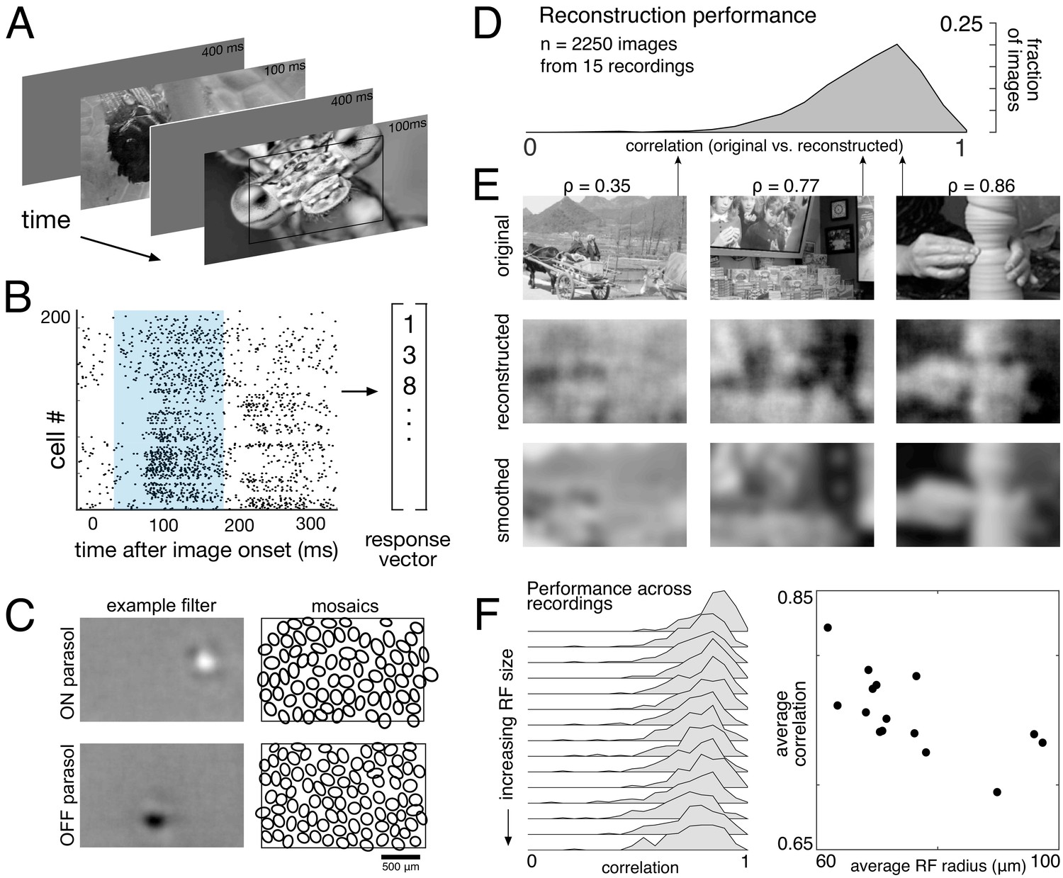
Linear reconstruction from ON and OFF parasol cell responses.
(A) Visual stimulus: static images from the ImageNet database were displayed for 100 ms, with 400 ms of gray between. The thin black rectangle indicates the central image region shown in C and E. (B) Example population response: each entry corresponds to the number of spikes from one RGC in a 150 ms window (shown in blue) after the image onset. (C) Left: Examples of reconstruction filters for an ON (top) and OFF (bottom) parasol cell. Right: RF locations for the entire population of ON (top) and OFF (bottom) parasol cells used in one recording. (D) Reconstruction performance (correlation) across all recordings. (E) Example reconstructions for three representative scores (middle row), compared to original images (top row) and smoothed images (bottom row), from the same recording and at the same scale as shown in C. (F) Reconstruction performance across 15 recordings. Left: Distributions of scores across images for each recording, ordered by average receptive field (RF) size. Right: Average reconstruction performance vs. average RF radius (ρ=−0.7). Source files for D and F are available in Figure 1—source data 1.
-
Figure 1—source data 1
Linear reconstruction from ON and OFF parasol cell responses.
This zip file contains the code and data for Figure 1D and F, which show the distribution of reconstruction scores across recordings, as well as the relationship between reconstruction performance and receptive field (RF) size.
- https://cdn.elifesciences.org/articles/58516/elife-58516-fig1-data1-v2.zip
Figure 2
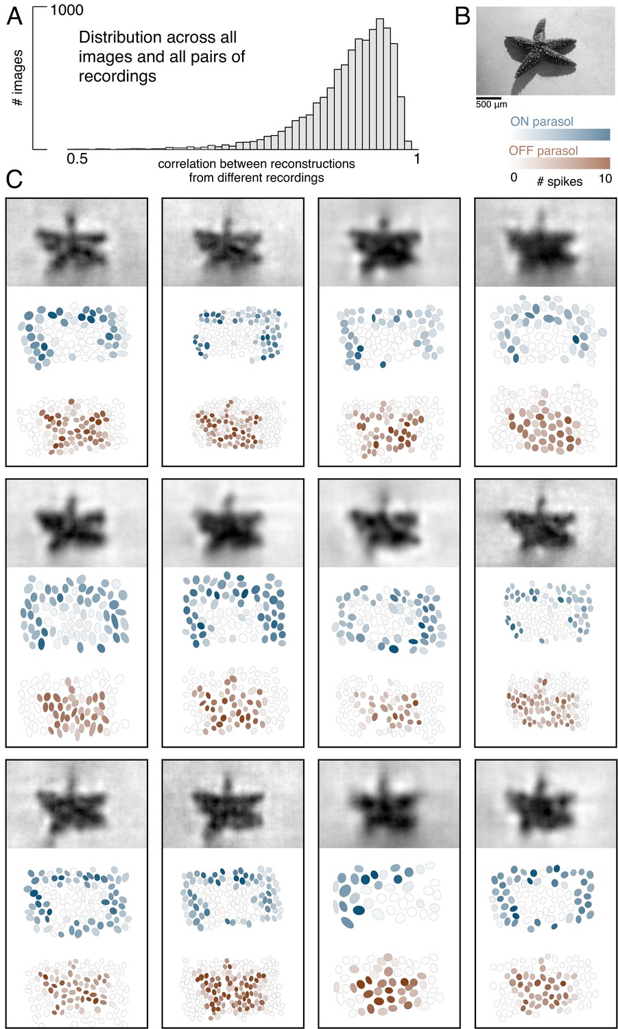
Visual representation across retinas.
(A) Distribution of correlation between reconstructed images from different recordings, across 150 images and 66 pairs of recordings. (B) Example image. (C) Across 12 recordings, reconstructed images (top, averaged across trials), ON (middle, blue) and OFF (bottom, orange) parasol responses, shown as the mosaic of Gaussian RF fits shaded by the spike count in response to this image. Source files for A are available in Figure 2—source data 1.
-
Figure 2—source data 1
Visual representation across retinas.
This zip file contains the code and data for Figure 2A, which shows the similarity of reconstructed images across separate recordings.
- https://cdn.elifesciences.org/articles/58516/elife-58516-fig2-data1-v2.zip
Figure 3
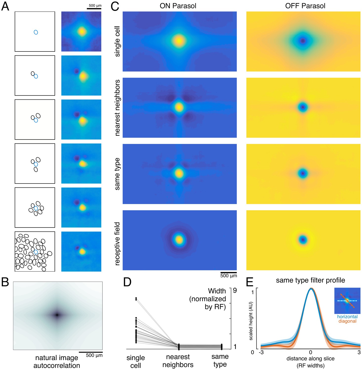
Effect of the population on the visual message.
(A) The reconstruction filter of a single cell as more neighboring cells are included in the reconstruction. Left: receptive fields (RFs) of cells in reconstruction, with the primary cell indicated in blue. Right: Filter of the primary cell. (B) Autocorrelation structure of the natural images used here. (C) Average ON (left) and OFF (right) parasol cell filters for a single recording. From top to bottom: reconstruction from a single cell, reconstruction from that cell plus all nearest neighbors, reconstruction from that cell plus all cells of the same type, and that cell’s RF. (D) Filter width, normalized by the RF width. (E) Profiles of the same type filters in the horizontal (orange) and diagonal (blue) directions. Average (bold) +/- standard deviation (shaded region) across recordings. Source files for D and E are available in Figure 3—source data 1.
-
Figure 3—source data 1
Effect of the population on the visual message.
This zip file contains the code and data for Figure 3D and E, which show how the visual message changes depending on other RGCs. This includes the widths and profiles of the reconstruction filters.
- https://cdn.elifesciences.org/articles/58516/elife-58516-fig3-data1-v2.zip
Figure 4
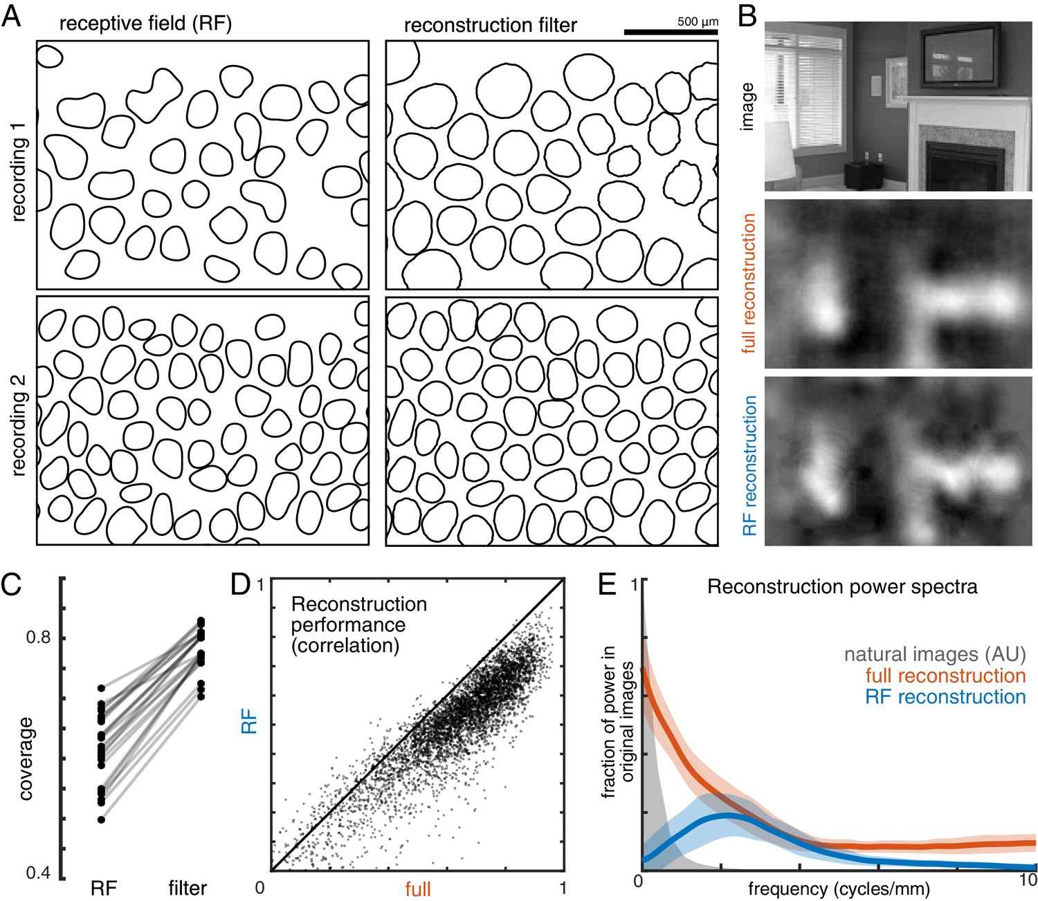
Effect of visual message on reconstruction.
(A) Receptive field (RF, left) and reconstruction filter (right) contours for two sample recordings. (B) Reconstruction of an image (top) using the full, fitted filters (middle) and using scaled RFs (bottom). (C) Comparison of RF and filter coverage for ON and OFF parasol cells across 12 recordings. (D) Comparison of reconstruction performance using scaled RFs or using full, fitted filters, across n = 4800 images from eight recordings. (E) Power in the reconstructed images (as a fraction of power in the original image) using fitted filters (orange) or scaled RFs (blue). Average (bold) +/- standard deviation (shaded region) across eight recordings. The original power structure of the natural images is shown in gray and has arbitrary units. Source files for C, D, and E are available in Figure 4—source data 1.
-
Figure 4—source data 1
Effect of the visual message on reconstruction.
This zip file contains the code and data for Figure 4C, D and E, which compare the full and receptive field (RF) reconstructions. This includes the coverage values for the RFs, the filters, and the expanded RFs, as well as the full and RF reconstruction scores, and the power spectra of the full and RF reconstructions.
- https://cdn.elifesciences.org/articles/58516/elife-58516-fig4-data1-v2.zip
Figure 5
Effect of other cell types on the visual message.
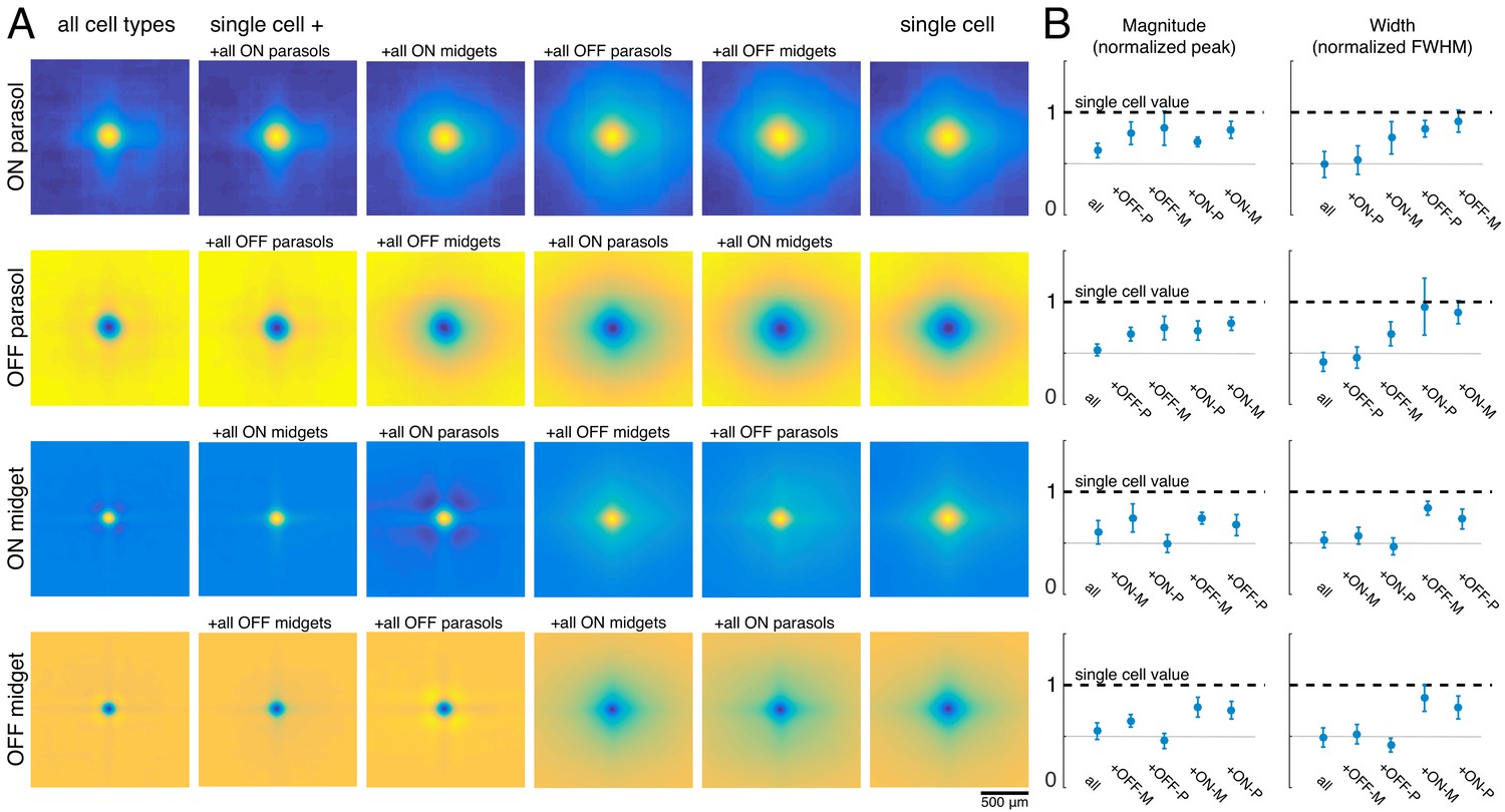
(A) Average reconstruction filters for ON parasol (top row), OFF parasol (second row), ON midget (third row), and OFF midget (bottom row) cells for one recording. Left to right: including all cell types, all cells of the same type, all cells of the same polarity but opposite class, all cells of the opposite polarity but the same class, all cells of opposite polarity and class, and no other cell types. (B) Comparison of magnitude (left) and width (right) of average reconstruction filters across conditions, normalized by the features of the single-cell filter. Average +/- standard deviation across recordings is plotted (parasol: n = 11 recordings, midget: n = 5 recordings). Rows correspond to cell types as in A. Source files for B are available in Figure 5—source data 1.
-
Figure 5—source data 1
Effect of other cell types on the visual message.
This zip file contains the code and data for Figure 5B, which compares the magnitude and width of the filters when other cell types are included in the reconstruction.
- https://cdn.elifesciences.org/articles/58516/elife-58516-fig5-data1-v2.zip
Figure 6
Contributions of ON and OFF parasol cells.
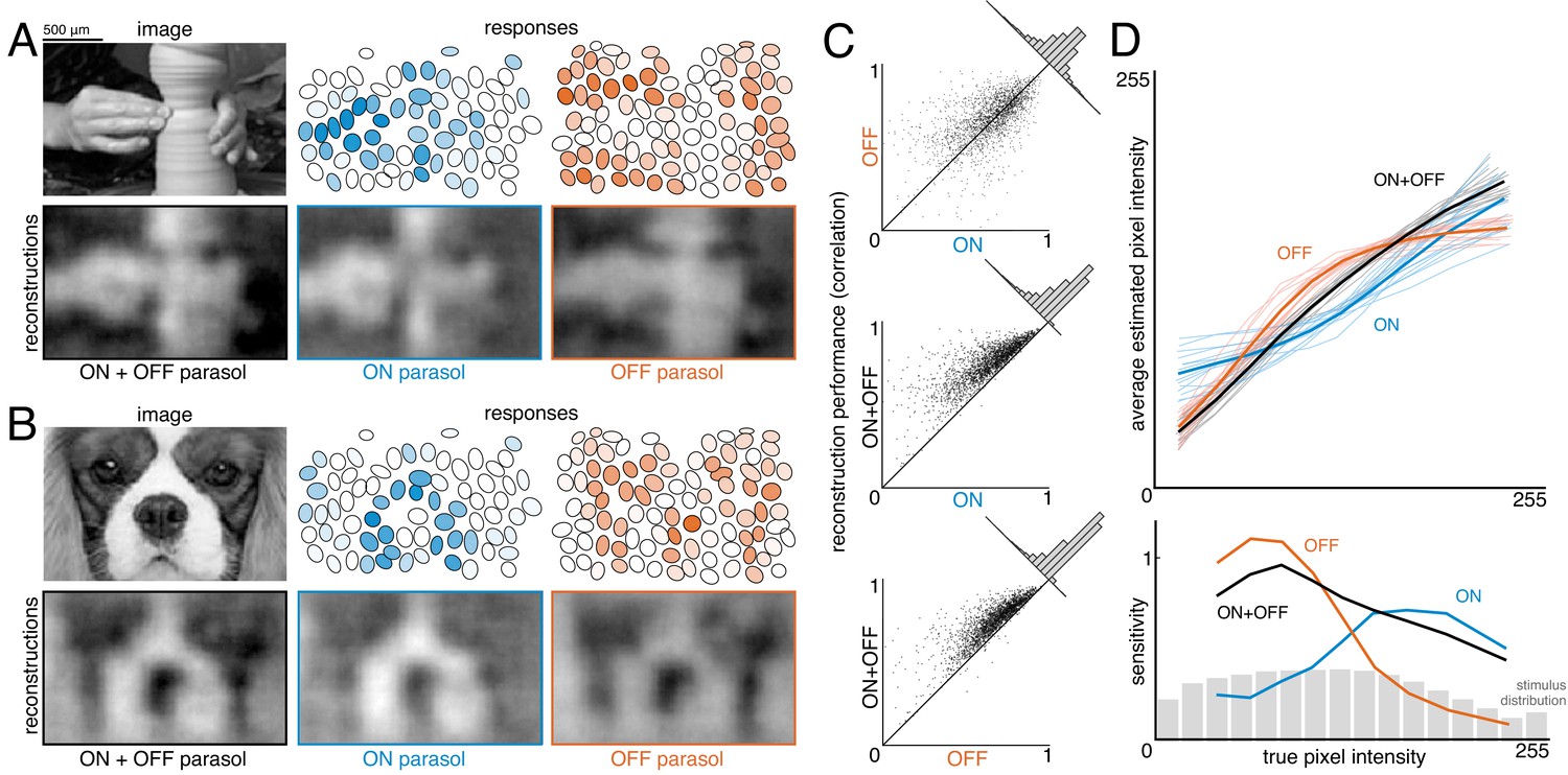
(A,B) Example images, responses, and reconstructions from ON and OFF parasol cells. Top left: original image. Top right: Parasol cell mosaics shaded by their response value (ON - blue, middle, OFF - orange, right). Bottom left: reconstruction from both cell types. Bottom right: reconstruction from just ON (blue, middle) or just OFF (orange, right) parasol cells. (C) Reconstruction performance for ON vs. OFF (top), both vs. ON (middle), and both vs. OFF (bottom), with n = 2250 images from 15 recordings. (D) Average estimated pixel intensity (top) and sensitivity (bottom, defined as Δaverage estimated pixel intensity/Δtrue pixel intensity) vs. true pixel intensity for ON (blue), OFF (orange), and both (black). Individual recordings are shown in the top plot, with the average in bold. Source files for C and D are available in Figure 6—source data 1.
-
Figure 6—source data 1
Contributions of ON and OFF parasol cells.
This zip file contains the code and data for Figure 6C and D, which compare the reconstructions from ON and OFF parasol cell responses. This data includes the performance scores for reconstructions from ON and OFF parasol cell responses, as well as the binned true and estimated pixel values.
- https://cdn.elifesciences.org/articles/58516/elife-58516-fig6-data1-v2.zip
Figure 7
Contributions of the parasol and midget cell classes.
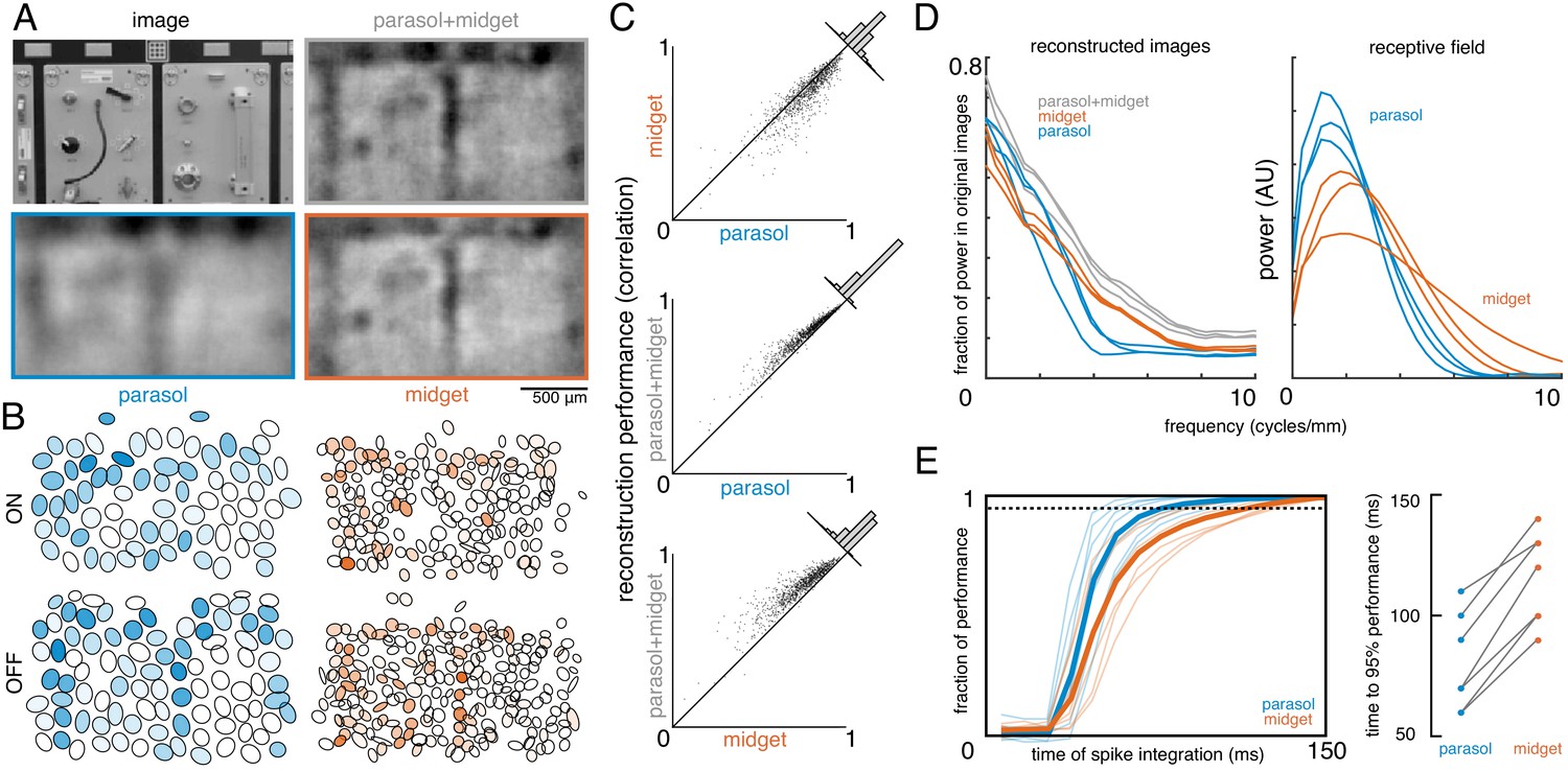
(A) Example image and reconstructions for parasol and midget cells. Top left: original image. Top right: reconstruction with parasol and midget cells (gray). Bottom left: reconstruction with only parasol cells (blue). Bottom right: reconstruction with only midget cells (orange). (B) Cell type mosaics shaded by their response values, for ON (top) and OFF (bottom) parasol cells (left, blue) and midget cells (right, orange). (C) Reconstruction performance for midget vs. parasol (top), both vs. parasol (middle), and both vs. midget (bottom). (D) Power in the reconstructed images as a fraction of power in the original image (left) and receptive fields (right) for parasol cells (blue), midget cells (orange), and both types (gray) for each of three recordings. (E) Left: Fraction of peak reconstruction performance with increasing spike integration times for parasol (blue) and midget (orange) cells, with averages across recordings shown in bold. Dotted line indicates 95% performance. Right: Time to 95% performance for parasol and midget reconstructions across seven recordings. Source files for C, D, and E are available in Figure 7—source data 1.
-
Figure 7—source data 1
Contributions of the parasol and midget cell classes.
This zip file contains the code and data for Figure 7C, D and E, which compare the reconstructions from parasol and midget cell responses. This data includes the performance scores for reconstructions from parasol and midget cell responses, as well as the power spectra of the resulting images, and the time required to reach 95% reconstruction performance.
- https://cdn.elifesciences.org/articles/58516/elife-58516-fig7-data1-v2.zip
Figure 8
Effect of noise correlations.
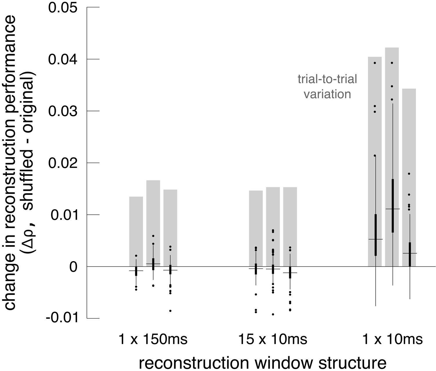
The change in reconstruction performance (Δρ) when using shuffled data for three scenarios: one 150 ms window, fifteen 10 ms windows, and one 10 ms window. Black bars show median +/- interquartile range for three recordings (each shown separately). Gray bars show the standard deviation in the reconstruction performance across trials. Source files are available in Figure 8—source data 1.
-
Figure 8—source data 1
Effect of noise correlations.
This zip file contains the code and data for Figure 8, which shows the effects of noise correlations on reconstruction performance.
- https://cdn.elifesciences.org/articles/58516/elife-58516-fig8-data1-v2.zip
Figure 9
Nonlinear reconstruction.
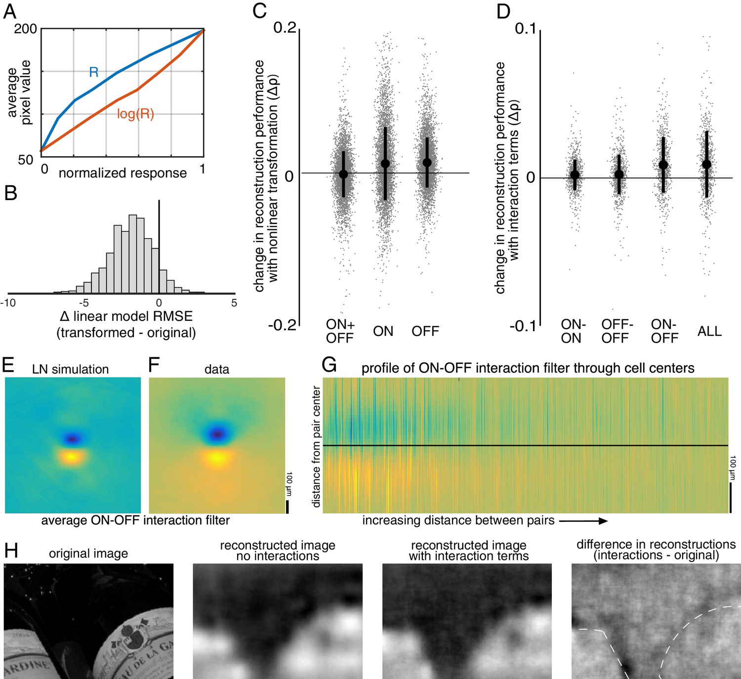
(A) Average pixel value in receptive field center vs. original response (blue) and transformed response (orange). (B) Distribution (across n = 2225 cells from 15 recordings) of the change in RMSE of a linear model (mapping from response to pixel value) when using the transformed response. (C) Change in reconstruction performance (correlation) when using transformed responses (log(R)) for reconstruction with either ON and OFF parasol cells, only ON parasol cells, or only OFF parasol cells. Individual images (n = 300 from each of the 15 recordings) are plotted in gray with jitter in the x-direction. The black bars represent mean +/- standard deviation, and the standard error is smaller than the central dot. (D) Change in reconstruction performance (correlation) when including interaction terms. Individual images (n = 300 from each of the three recordings) are plotted in gray with jitter in the x-direction. The black bars represent mean +/- standard deviation, and the standard error is smaller than the central dot. (E,F) Average reconstruction filters corresponding to ON-OFF type interactions, centered and aligned along the cell-to-cell axis, for simulation (E) and data (F). (G) 1D Profiles of all ON-OFF interaction filters through the cell-to-cell axis, sorted by distance between the pair. (H) Example image (left), reconstructions with and without interaction terms (middle), and difference between the reconstructions, with dotted lines indicating edges (right). Source files for B, C, and D are available in Figure 9—source data 1.
-
Figure 9—source data 1
Nonlinear reconstruction.
This zip file contains the code and data for Figures 9B, C and D, which show the effects of using a static nonlinear transformation, and of including nonlinear interaction terms.
- https://cdn.elifesciences.org/articles/58516/elife-58516-fig9-data1-v2.zip
Figure 10
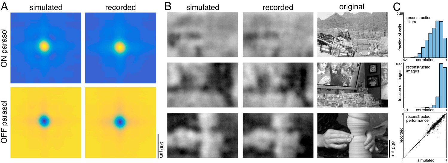
Comparison to simulated spikes.
(A) Average reconstruction filters calculated from spikes simulated using linear-nonlinear models (left) or recorded (right). (B) Images reconstructed from simulated (left) or recorded (middle) spikes, compared to the original images (right). (C) Comparison of reconstructions with recorded and simulated spike counts: filters (top; ρ=0.84 +/- 0.09 across 2225 parasol cells from 15 recordings), reconstructed images (middle; ρ=0.93 +/- 0.04 across n = 2250 images from 15 recordings), and performance (bottom; simulated: ρ=0.79 +/- 0.11; recorded: ρ=0.78 +/- 0.11; Δρ=−0.003 +/- 0.03; across 2250 images from 15 recordings). Source files for C are available in Figure 10—source data 1.
-
Figure 10—source data 1
Comparison to simulated spikes.
This zip file contains the code and data for Figure 10C, which compares reconstruction using recorded and simulated RGC responses.
- https://cdn.elifesciences.org/articles/58516/elife-58516-fig10-data1-v2.zip
Figure 11
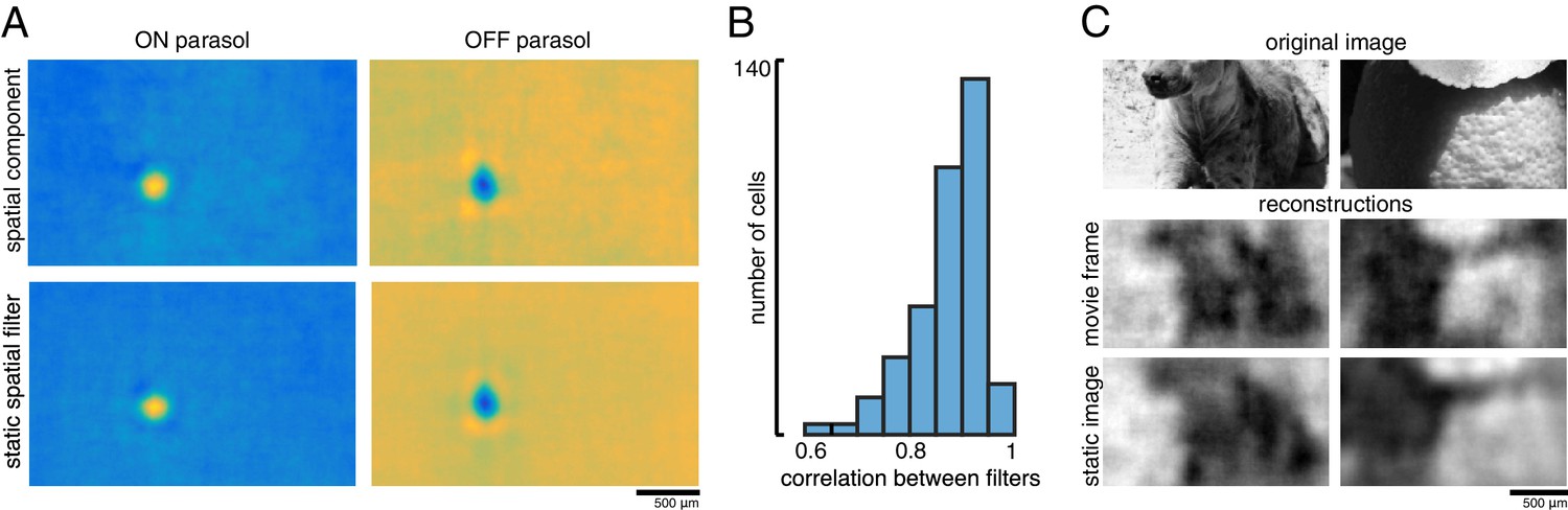
Spatiotemporal reconstruction.
(A) Examples of the spatial components extracted from the spatiotemporal reconstruction filter (top) and the static spatial reconstruction filters (bottom) for an ON (left) and OFF (right) parasol cell. (B) Correlation between spatial component and static filter (ρ=0.87 +/- 0.07 across n = 351 cells from three recordings). (C) Example reconstructions of movie frames and of static images. Source files for B are available in Figure 11—source data 1.
-
Figure 11—source data 1
Spatiotemporal reconstruction.
This zip file contains code and data for Figure 11B, which compares static and spatiotemporal reconstruction filters.
- https://cdn.elifesciences.org/articles/58516/elife-58516-fig11-data1-v2.zip
Figure 12
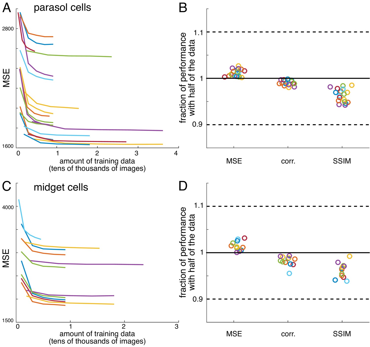
Verification of data sufficiency.
(A) Performance of reconstructions from parasol cell responses as a function of the amount of training data, for 19 recordings (colors). (B) Fraction of performance of reconstructions from parasol cell responses (MSE, correlation, and SSIM) achieved with half of the training data for each recording. (C,D) Same as A, B for reconstructions from midget cell responses for 12 recordings (colors).
Figure 13
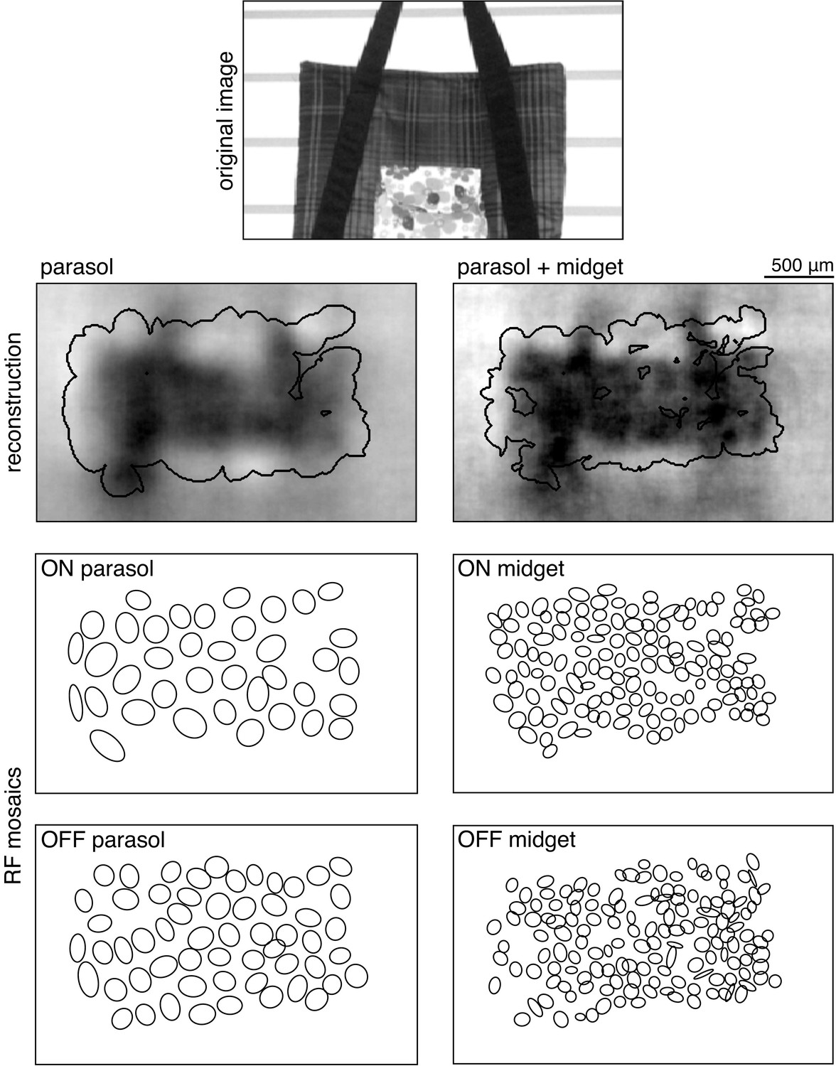
Selection of analysis region.
Reconstruction performance on a sample image (top) is measured by comparing the regions inside the contours shown on the reconstructions in the second row. These contours were obtained using the receptive field mosaics (bottom two rows) of parasol cells, or of both parasol and midget cells, as described in Image region selection. Here, OFF midget cells had the least complete mosaic, so the included region was most limited by their coverage. The bounding boxes mark the extent of the visual stimulus.
Additional files
Download links
A two-part list of links to download the article, or parts of the article, in various formats.
Downloads (link to download the article as PDF)
Open citations (links to open the citations from this article in various online reference manager services)
Cite this article (links to download the citations from this article in formats compatible with various reference manager tools)
Reconstruction of natural images from responses of primate retinal ganglion cells
eLife 9:e58516.
https://doi.org/10.7554/eLife.58516


