Sniff-synchronized, gradient-guided olfactory search by freely moving mice
- Department of Biology and Institute of Neuroscience, University of Oregon, United States
- Department of Psychology and Institute of Neuroscience, University of Oregon, United States
- Computational & Biological Learning Lab, University of Cambridge, United Kingdom
Figures
Figure 1 with 2 supplements
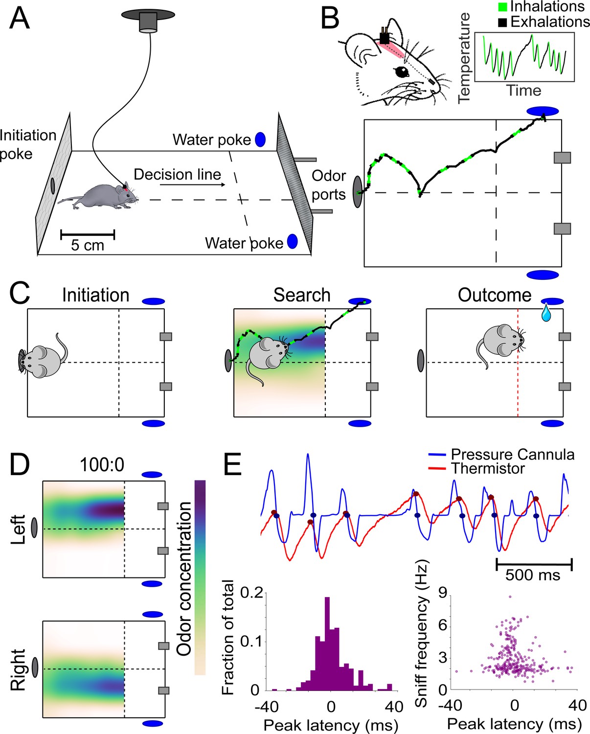
Behavioral assay for freely moving olfactory search.
(A) Diagram of experimental chamber where mice are tracked by an overhead camera while performing olfactory search. (B) Top: nose and head positions are tracked using red paint at the top of the head. Sniffing is monitored via an intranasally implanted thermistor. Bottom: example of sniffing overlaid on a trace of nose position across a single trial. (C) Diagram of trial structure. Initiation. Mice initiate a trial via an initiation poke (gray oval). Search. Odor is then released from both odor ports (gray rectangles) at different concentrations. Outcome. Mice that cross the decision line (red) on the side delivering the higher concentration as tracked by the overhead camera receive a reward at the corresponding water port (blue ovals). (D) Colormaps of average odor concentration across ~15 two-second trials captured by a 7 × 5 grid of sequential photoionization detector recordings. Rows represent side of stimulus presentation (left or right). Odor concentrations beyond the decision line were not measured. (E) Comparison of sniff recordings taken with an intranasally implanted thermistor and intranasally implanted pressure cannula. These are implanted on the same mouse in different nostrils. Top: example trace of simultaneous pressure cannula (blue) and thermistor (red) recordings with inhalation points (as detected in all future analyses) overlaid on the traces in their respective colors. Bottom left: histogram of peak latencies (pressure inhalation onset – thermistor inhalation onset). 14/301 inhalations (4.7%) were excluded as incorrect sniff detections. These were determined as incorrect because they fell more than 2 standard deviations outside the mean in peak latency (mean = 1.61585 ms, SD = ±14.93223 ms). Bottom right: peak latencies, defined as the difference between pressure inhalation onset and thermistor inhalation onset, plotted against instantaneous sniff frequency.
Figure 1—figure supplement 1
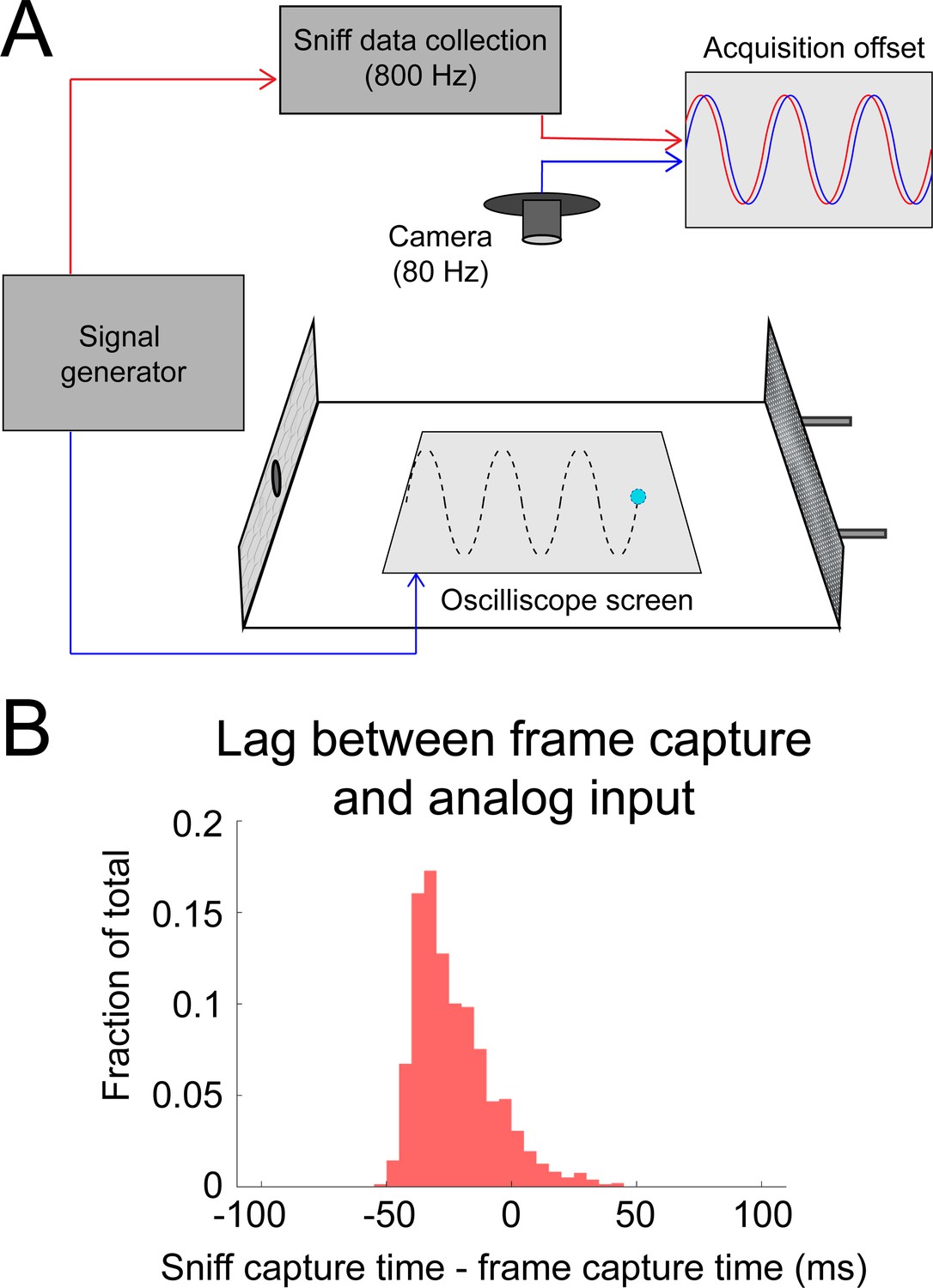
Calibrating alignment of video frames with sniff signal.
(A) Sinusoidal signals (5, 8, 10, and 15 Hz) were simultaneously sent to the analog input channel (used to capture sniffing) and to a phosphor-display oscilloscope (Tektronix). The display of the oscilloscope was reflected by mirrors to allow it to be video-captured inside the behavioral arena. (B) The timing relationship is given by the lag between peaks in the analog input channel and the vertical peaks in the position of the oscilloscope trace. Analog input led video frames by 23.5 ± 15.7 ms (mean ± sd; approximately two frames at 80 frames/s).
Figure 1—figure supplement 2
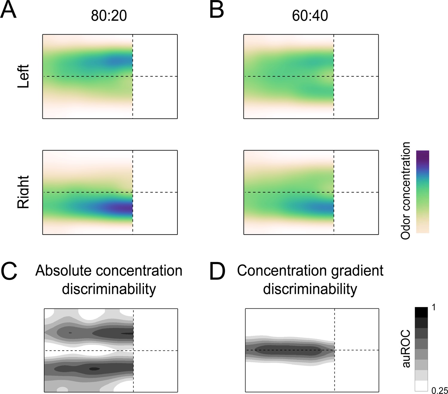
Characterizing the odor stimulus conditions.
(A) Colormaps of average odor concentration across ~15 two-second trials captured by a 7 × 5 grid of sequential photoionization detector (PID) recordings. -- Each row represents trial type (left correct or right correct). 80:20 odor condition (see Materials and methods: behavioral training: 80:20). (B) Same as (A), for the 60:40 odor condition (see Materials and methods: interleaved: 60:40). (C) Absolute concentration discriminability map based on PID recordings (see Materials and methods). Darker shades indicate regions where absolute concentrations are most discriminable according to ROC analysis (see Methods: Mapping the Olfactory Environment). Essentially, these regions downwind of the odor ports have the largest differences in absolute concentration between left and right trials. (D) Concentration gradient discriminability map based on PID recordings. Darker shades indicate regions where odor concentration gradient angles are most discriminable according to ROC analysis. Essentially, this region around the lateral midline of the arena has the largest differences in concentration gradient between left and right trials.
Figure 2 with 2 supplements
Mice use concentration gradient cues in turbulent flow to perform search.
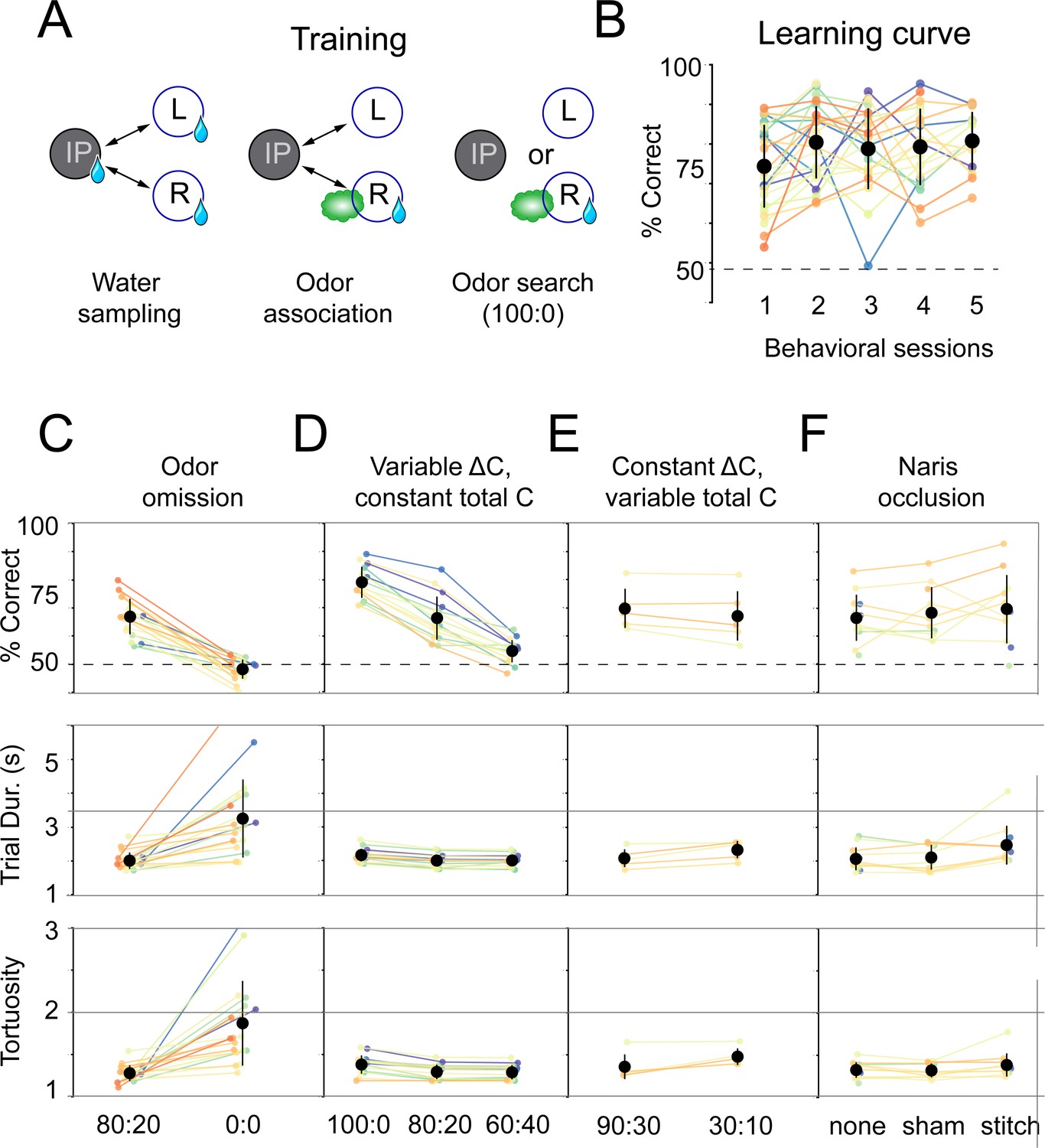
(A) Initial training steps. Water sampling. In this task, mice alternate in sequence between the initiation, left, and right nose pokes to receive water rewards. Odor association. Next, mice run the alternation sequence as above without water rewards released from the initiation poke, making its only utility to initiate a trial. Further, odor is released on the same side of water availability to create an association between odor and reward. Odor search. Here, mice initiate trials by poking the initiation poke. Odor is then randomly released from the left or right odor port. Correct localization (see Figure 1C, decision line) results in a water reward and incorrect is deterred by an increased inter-trial interval (ITI). (B) Performance curve across sessions for the odor search (100:0) training step (n = 26). (C–F) Session statistics for four different experiments. Each colored line is the average of an individual mouse across all sessions, black points are means across mice, and whiskers are ±1 standard deviation across mice. Top: percent of correct trials. Middle: average trial duration. Bottom: average path tortuosity (total path length of nose trajectory/shortest possible path length). (C) Odor omission. The 80:20 concentration ratio (Figure 1) and odor omission (0:0) conditions randomly interleaved across a session. Data shown includes all sessions for each mouse (n = 19). (D) Variable ΔC, Constant |C|. Three concentration ratio conditions (100:0, 80:20, 60:40) randomly interleaved across a session. Data shown includes all sessions for each mouse (n = 15). (E) Constant ΔC, Variable |C|. Concentration ratio conditions 90:30 and 30:10 randomly interleaved across a session (n = 5). Data shown for first session only. (F) Naris occlusion. 80:20 sessions for mice with no naris stitch, a sham stitch that did not occlude the nostril, and a naris stitch that occluded one nostril (n = 13). Data shown includes all naris occlusion sessions even if the mouse did not perform under every experimental condition.
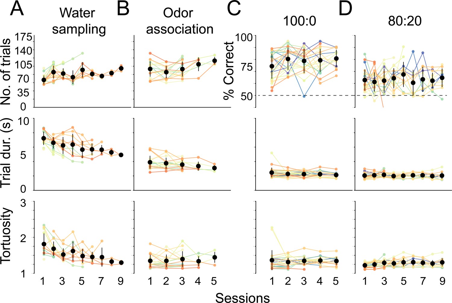
Figure 2—figure supplement 1
Session statistics across trainer sessions.
Individual mice are depicted by colored lines, average across mice are black points, and whiskers are ±1 standard deviation from the average across mice. Mice 2054–2062 did not have trainer 1 and 2 recorded (this accounts for increasing n), and mice were commonly removed from the experiment if they lost sniff signal (this accounts for the reducing n). Above: number of trials performed or percent of correct trials. Middle: average trial duration. Below: average trial path tortuosity (total path length/shortest possible path length). (A) Session statistics for the first trainer, water sampling (n = 19). (B) Session statistics for the second trainer, odor association (n = 19). (C) Session statistics for the third trainer, 100:0 or olfactory search (n = 26). Mice perform above 70% in first session. (D) Session statistics for final training step, 80:20, that preceded experiments shown in Figure 2 (n = 24).
Figure 2—figure supplement 2
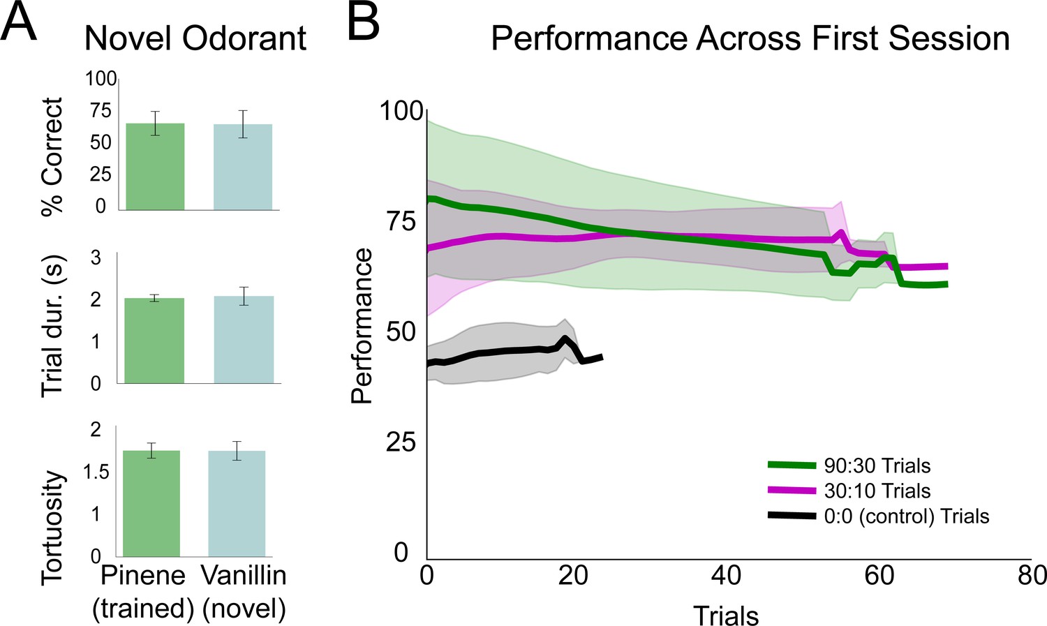
Mice generalize search task to novel odorants and variable |C| session.
(A) Performance, trial duration, and trial tortuosity (total path length/shortest possible path length) for the last session of pinene training in 80:20 and the first session of vanillin in 80:20 across mice (n = 3). (B) Grouped by stimulus condition (90:30, 30:10, 0:0), each line represents the rolling average across mice (window = 10) for the first session (n = 5). Shaded regions represent ±1 standard deviation.
Figure 3 with 1 supplement
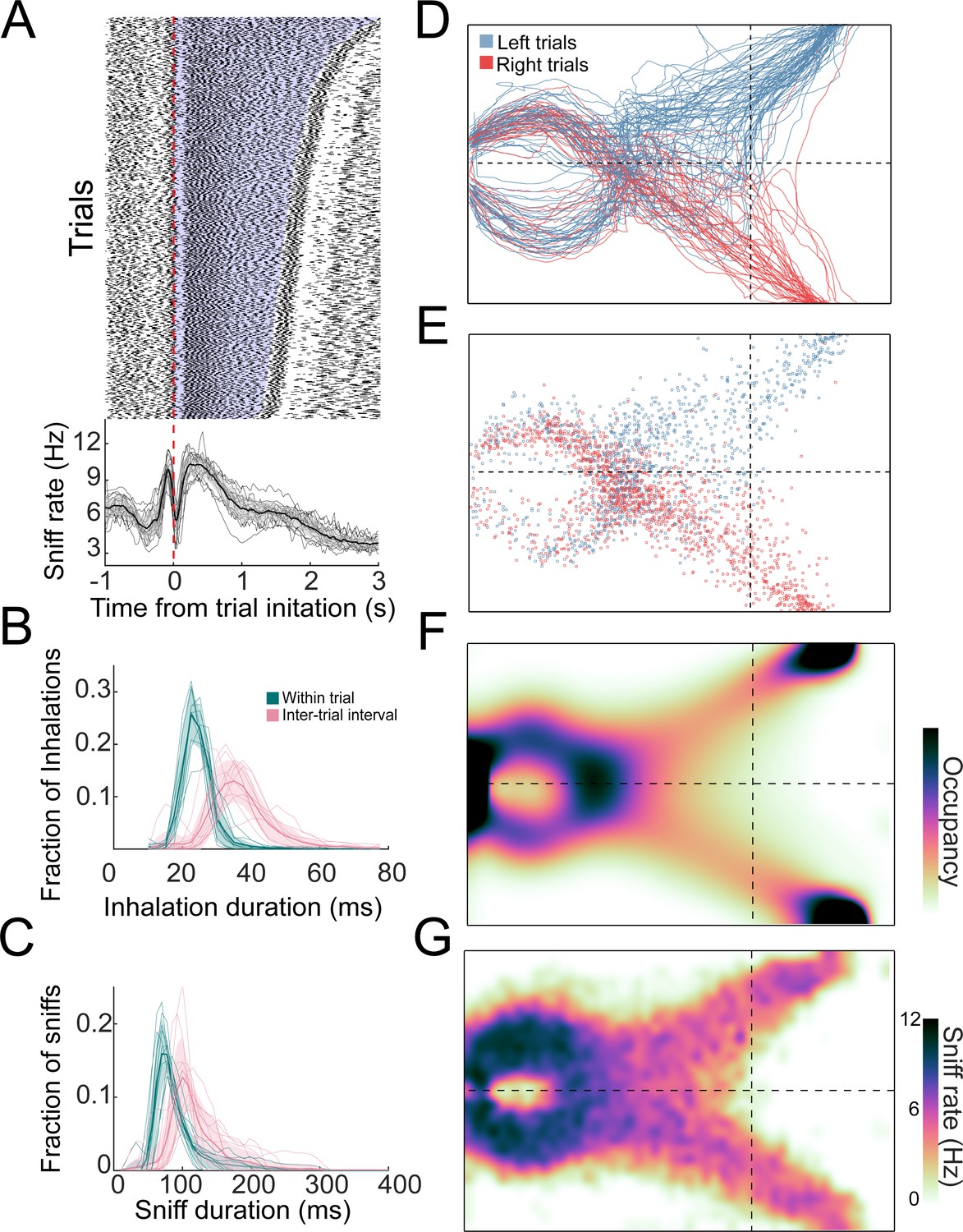
Distributions of sniffs and nose positions during search task.
(A) Above: sniff raster plot for three sessions. Each black point is an inhalation, each row is a trial aligned to trial initiation (dashed line). Rows are sorted by trial length. Blue region represents trial initiation to trial end. Below: mean instantaneous sniff rate across all trials for all mice aligned to time from trial initiation. Thin lines are individual mice, the thick line is the mean across mice, and shaded region is ±1 standard deviation. (B) Histogram of inhalation duration time across all mice (n = 11). Thick lines and shaded regions are mean and ±1 standard deviation, thin lines are individual mice. Green: within-trial sniffs; pink: inter-trial interval sniffs. (C) Histogram of sniff duration time across all mice (n = 11). (D) The nose traces of each trial across a single session, colored by chosen side. (E) Location of all inhalations across a single session, colored by chosen side. (F) Two-dimensional histogram of occupancy (fraction of frames spent in each 0.5 cm² bin). Colormap represents grand mean across mice (n = 19). (G) Grand mean sniff rate colormap across mice (n = 11).
Figure 3—figure supplement 1
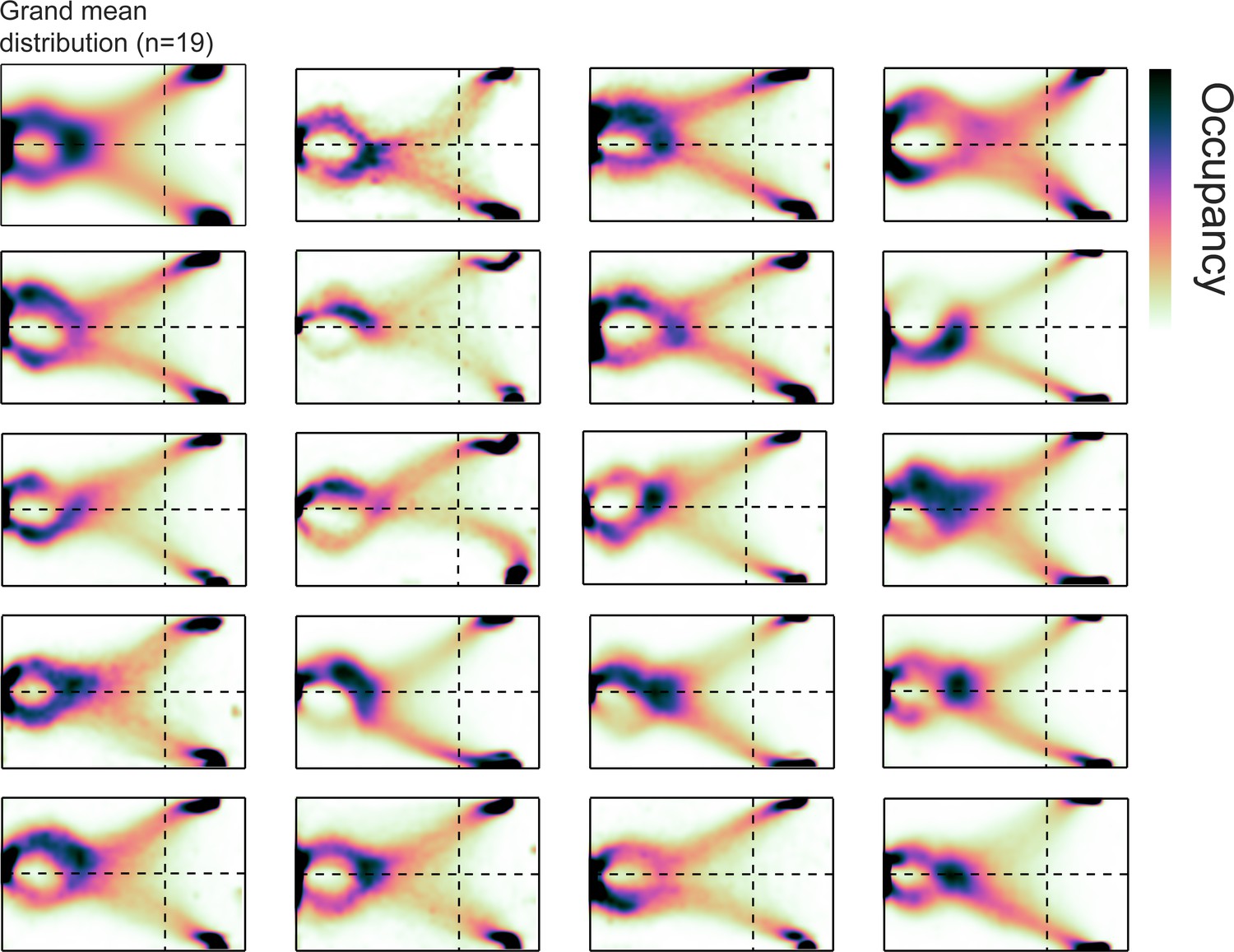
Idiosyncratic occupancy distributions across individual mice.
Two-dimensional histogram of occupancy (fraction of frames spent in each 0.5 cm² bin).
Figure 4

Quantifying kinematic parameters during olfactory search.
(A) Schematic of kinematic parameters. Left: two example frames from one mouse, with the three tracked points marked: tip of snout, back of head, and center of mass. (B) Quantified kinematic parameters: ‘nose speed’: displacement of the tip of the snout per frame (12.5 ms inter-frame interval). ‘Yaw velocity’: change in angle between the line segment connecting snout and head and the line segment connecting head and center of mass. Centrifugal movement is positive, centripetal movement is negative. ‘Z-velocity’: change in distance between tip of snout and back of head. Note that this measure confounds pitch angle and Z-axis translational movements. (C) Segments of example trajectories. Left: the trajectory of the nose during 1 s of trial time. Green: path during inhalations. Black: path during the rest of the sniff. Right: same for an inter-trial interval trajectory. (D) Traces of sniff and kinematic parameters during the time windows shown in (C). Color scheme as in (C).
Figure 5 with 2 supplements
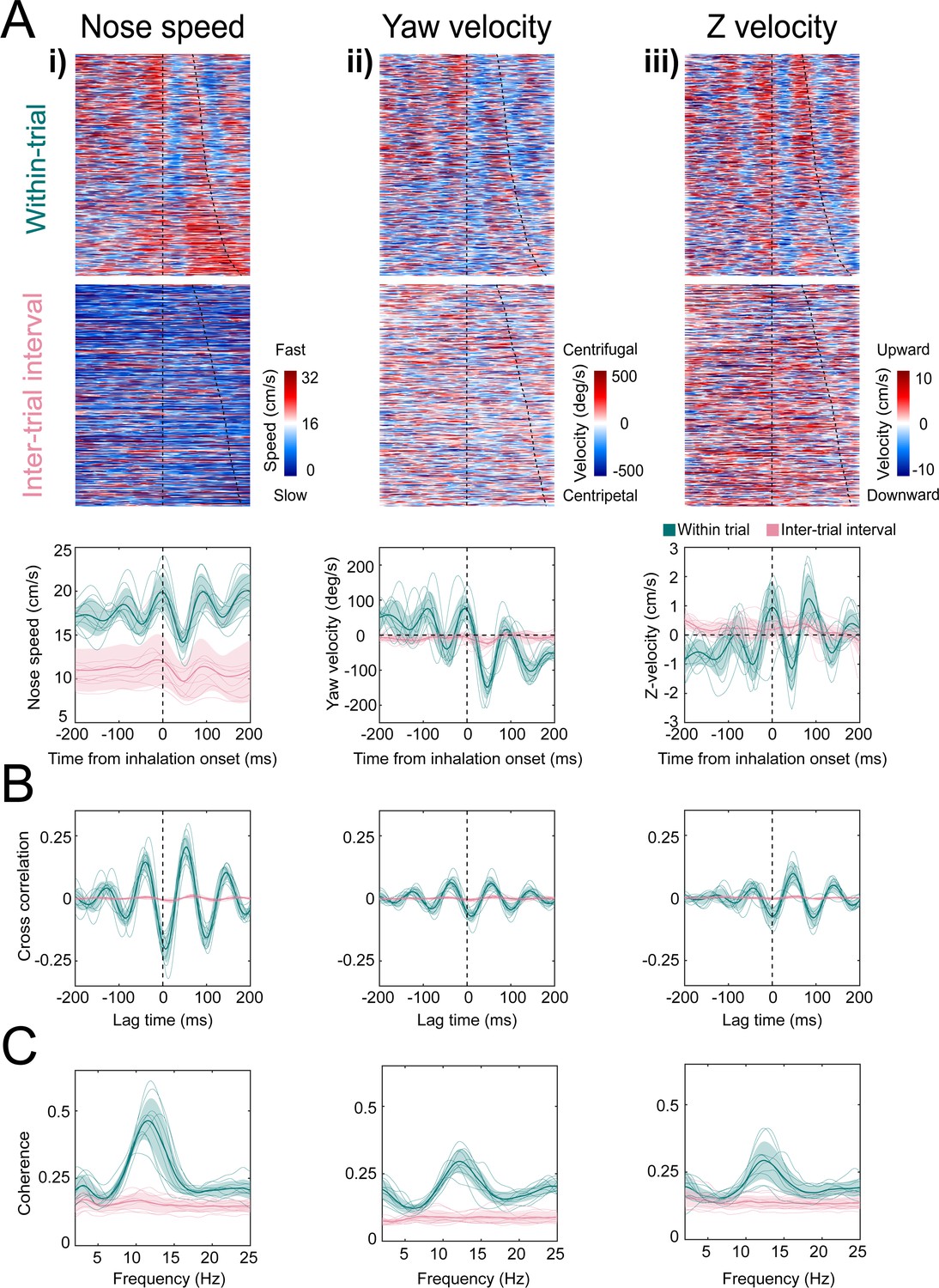
Kinematic rhythms synchronize with the sniff cycle selectively during olfactory search.
(i–iii) Nose speed, yaw velocity, and Z-velocity, respectively (see Figure 4 for definitions). (A) Top: color plot showing movement parameter aligned to inhalation onset for within-trial sniffs taken before crossing the decision line. Taken from one mouse, one behavioral session. Dotted line at time 0 shows inhalation onset, the second line demarcates the end of the sniff cycle, sorted by duration. Data are taken from one behavioral session. Middle: color plot showing each movement parameter aligned to inhalation onset for inter-trial interval sniffs taken before the first attempt at premature trial initiation. Bottom: sniff-aligned average of each movement parameter. Thin lines represent individual mice (n = 11), bolded lines and shaded regions represent the grand mean ± standard deviation. Green: within-trial sniffs; pink: inter-trial interval sniffs. (B) Normalized cross-correlation between movement parameter and sniff signal for the same sniffs as above. (C) Spectral coherence of movement parameter and sniff signal for the same sniffs as above.
Figure 5—figure supplement 1
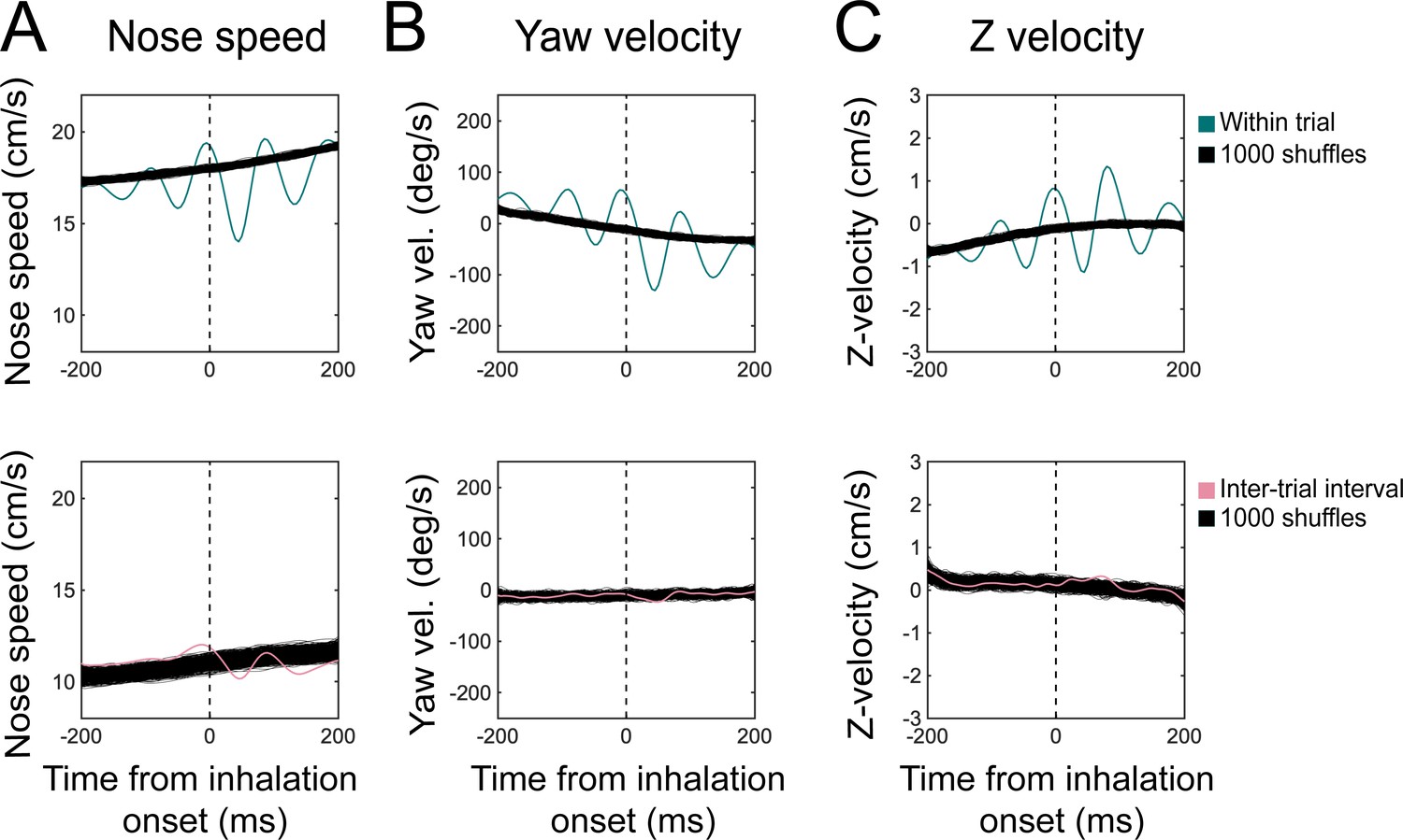
Sniff synchronization shuffle test.
Sniff-aligned grand mean (n = 11 mice) of (A) nose speed, (B) yaw velocity, and (C) Z-velocity for within-trial (top) and inter-trial interval (bottom) sniffs, overlaid on 1000 iterations of trial-shuffled grand means. Thin black lines represent individual iterations, all of which are shown.
Figure 5—figure supplement 2
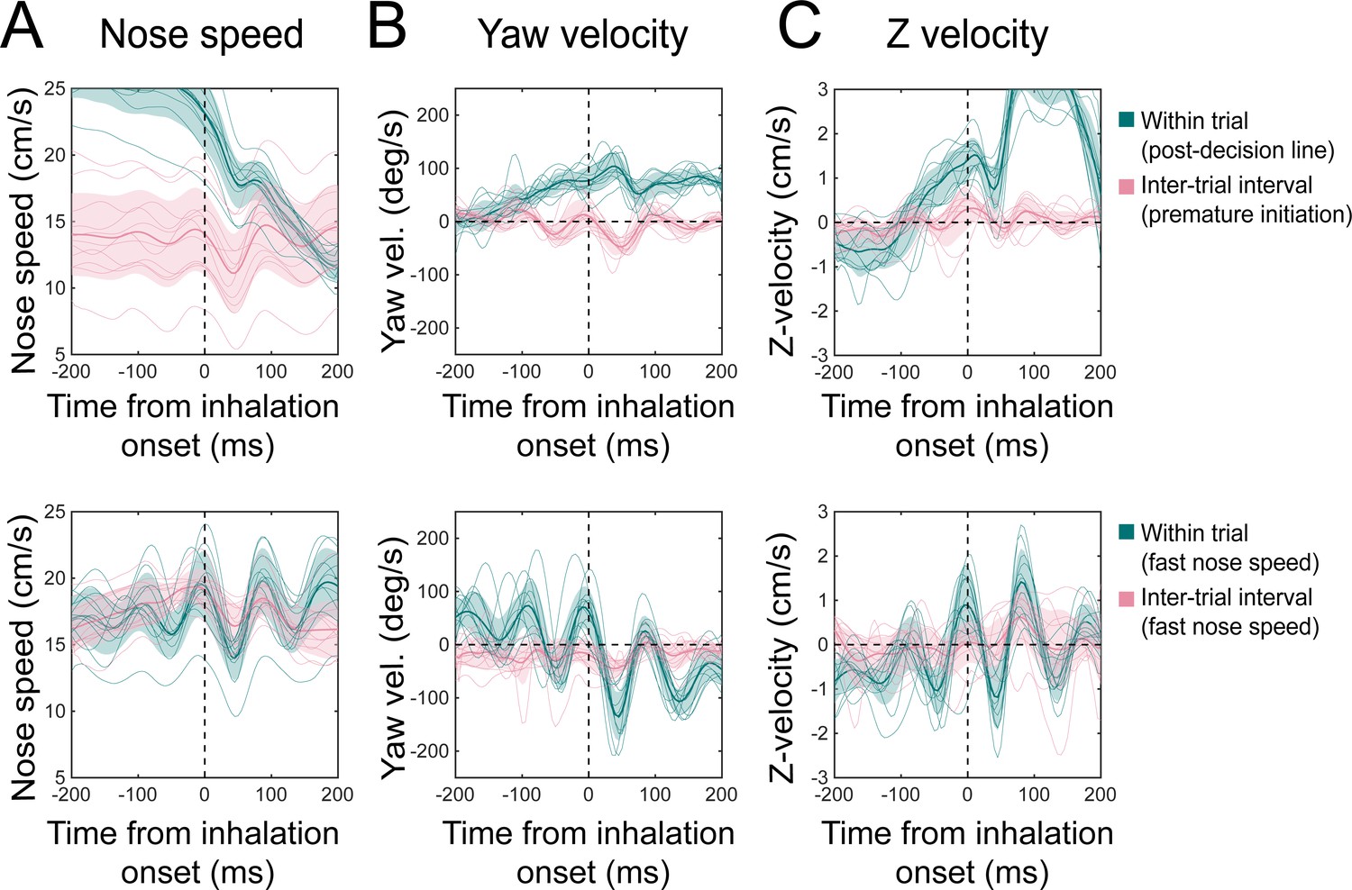
Kinematic rhythms for premature initiations during the inter-trial interval and between decision line and reward port during trials.
Sniff-aligned average of (A) nose speed, (B) yaw velocity, and (C) Z-velocity. Thin lines represent individual mice (n = 11), bolded lines and shaded regions represent the grand mean ± standard deviation. Top: green: within-trial sniffs from the time between crossing the decision line and entering the reward port. Pink: inter-trial interval sniffs from the time between the first premature trial initiation attempt and the successful initiation of the next trial. Bottom: green: within-trial sniffs at nose speeds above the threshold 15 cm/s. Pink: inter-trial interval sniffs at nose speeds above the threshold 15 cm/s.
Figure 6 with 5 supplements
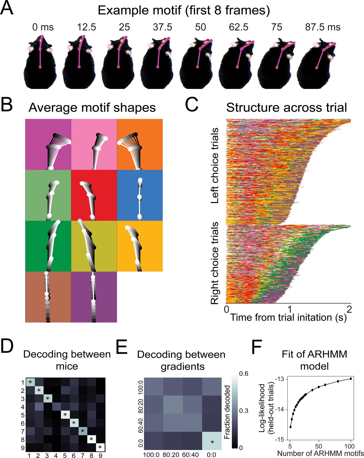
Recurring movement motifs are sequenced diversely across mice and consistently across stimuli.
(A) Eight example frames from one instance of a behavioral motif with tracking overlaid. (B) Average motif shapes. Dots and lines show the average time course of posture for eight frames of each of the 11 motifs (n = 9 mice). All instances of each motif are translated and rotated so that the head is centered and the head-body axis is oriented upward in the first frame. Subsequent frames of each instance are translated and rotated the same as the first frame. Time is indicated by color (dark to light). Background color in each panel shows the color assigned to each motif. (C) Across-trial motif sequences for two behavioral sessions for one mouse. Trials are separated into trials where the mouse chose left and those in which the mouse chose right. Trials are sorted by duration. Both correct and incorrect trials are included. Color scheme as in (B). (D) Linear classifier analysis shows that mice can be identified from motif sequences on a trial-by-trial basis. Grayscale represents the fraction of trials from a given mouse (rows) that are decoded as belonging the data of a given mouse (columns). The diagonal cells represent the accuracy with which the decoded label matched the true label, while off-diagonal cells represent trials that were mislabeled by the classifier. Probabilities along rows sum to 1. Cells marked with asterisks indicate above chance performance (label permutation test, p<0.01). (E) Linear classifier analysis identifies odor omission trials above chance, but does not discriminate across odor concentration ratios (n = 9 mice). (F) Cross-validated log-likelihood (evaluated on trials not used for model fitting) for fit auto-regressive hidden Markov model (AR-HMM) models with different numbers of motifs, S, shows that model log-likelihood does not peak or plateau up to S = 100.
Figure 6—figure supplement 1
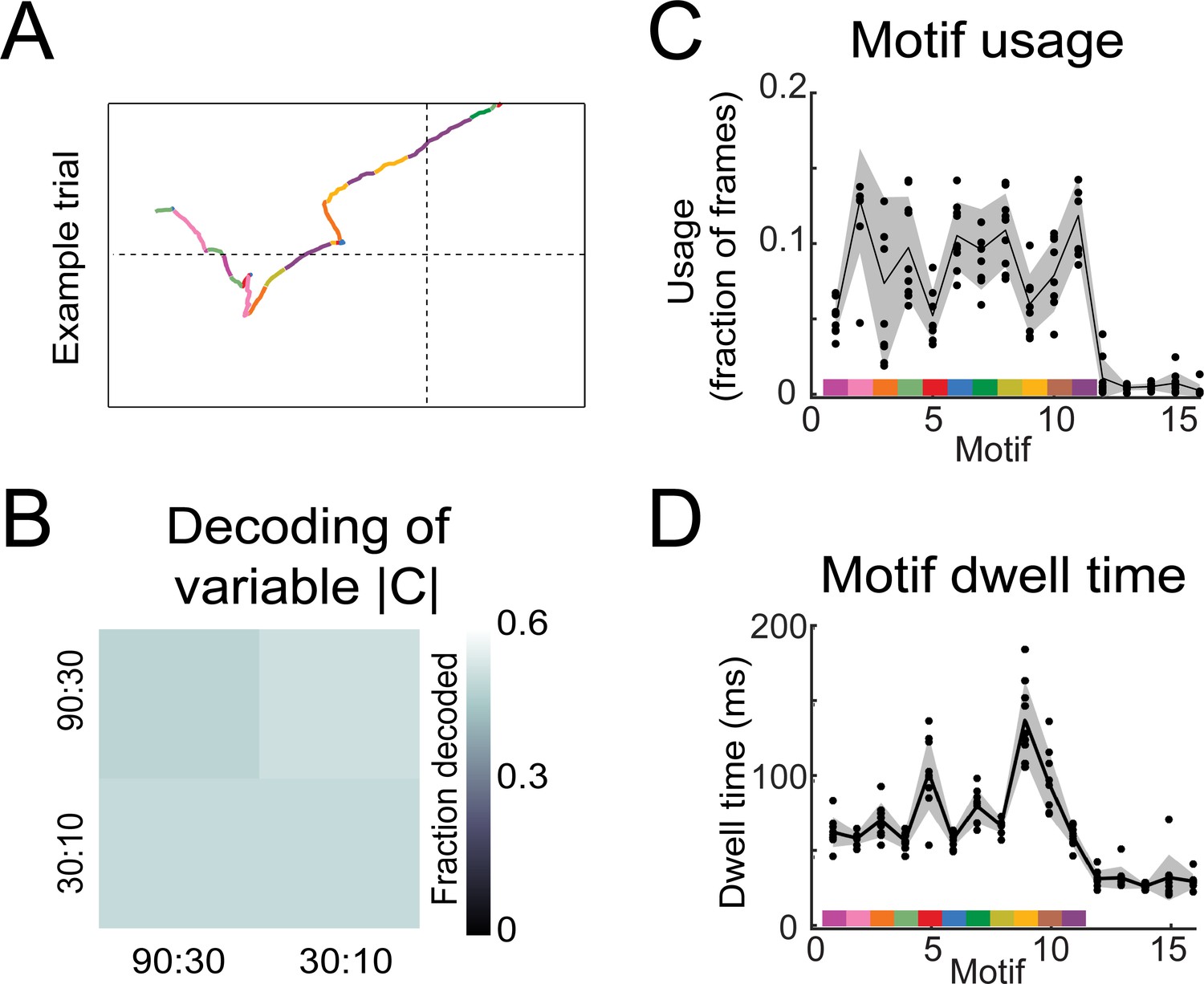
Motif statistics and examples and linear decoder results for 80:20 experiments.
(A) Example nose trace across a single trial colored by motif identity. (B) Linear decoder (Figure 6; Materials and methods: linear decoding section) results for Variable |C| experiments (n = 5). (C) Fraction of motif usage across all mice (n = 8) for the model with S = 16. Black points are individual mice, black line is average across mice, and shaded region is ±1 standard deviation. Colors on x-axis represent motifs used in analysis (Figure 6) and y-axis are fractions of frames that motif occupies. (D) The average dwell time of each motif across all mice (n = 8) for the model with S = 16. Black points are individual mice, black line is average across mice, and shaded region is ±1 standard deviation. Colors on x-axis represent motifs used in analysis (Figure 6) and y-axis are fractions of frames that motif occupies.
Figure 6—figure supplement 2
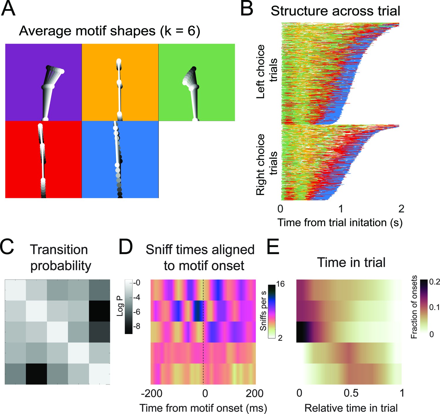
Motif shapes, sequences, transition matrices, and sniff synchronization for an auto-regressive hidden Markov model capped at a maximum of six states.
(A-E) As in Figure 6.
Figure 6—figure supplement 3
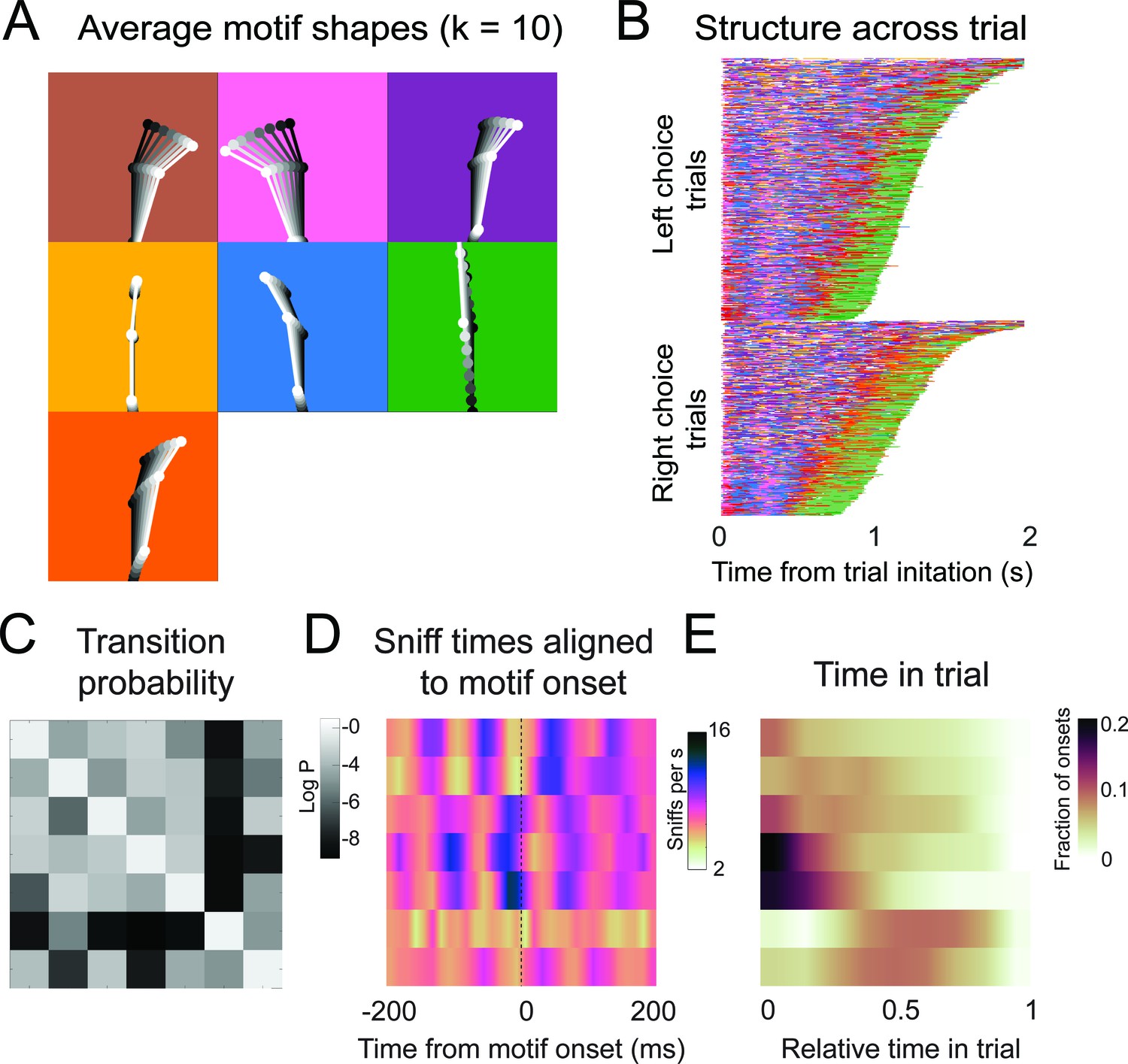
Motif shapes, sequences, transition matrices, and sniff synchronization for an auto-regressive hidden Markov model capped at a maximum of 10 states.
(A-E) As in Figure 6.
Figure 6—figure supplement 4
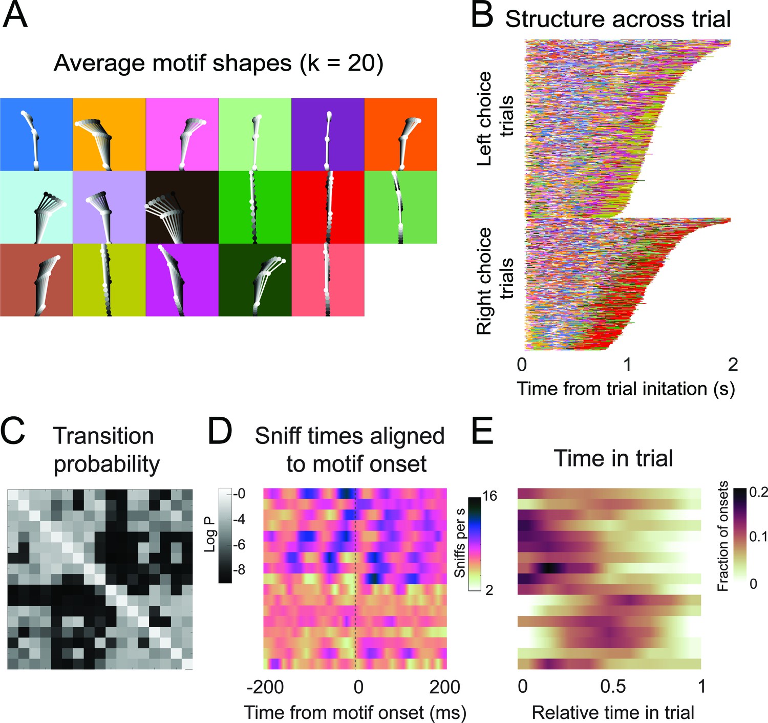
Motif shapes, sequences, transition matrices, and sniff synchronization for an auto-regressive hidden Markov model capped at a maximum of 20 states.
(A-E) As in Figure 6.
Figure 6—figure supplement 5
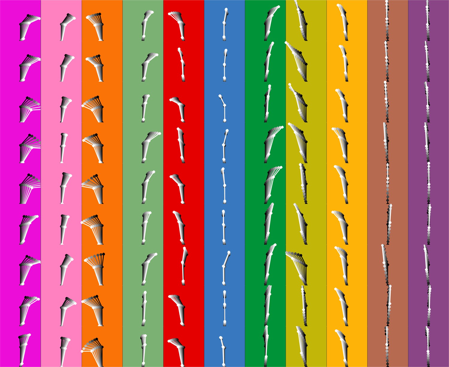
Motif shapes across individuals.
Average of first eight frames of the 11 commonly used motifs across individuals. Dots and lines show the average time course of posture for eight frames of each of the 11 motifs. All instances of each motif are translated and rotated so that the head is centered and the head-body axis is oriented upward in the first frame. Subsequent frames of each instance are translated and rotated the same as the first frame. Time is indicated by color (dark to light). Each color/column represents a single motif and each row an individual mouse.
Figure 7
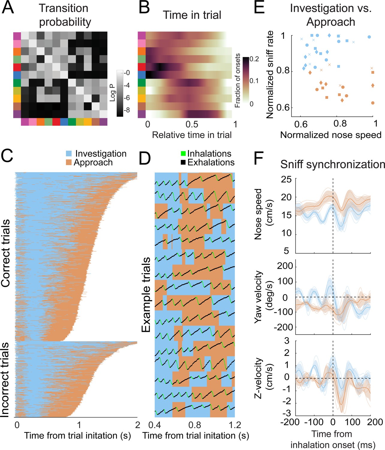
Behavioral motifs can be categorized into two distinct groups, which we putatively label as investigation (blue) and approach motifs (orange).
Colors in panel A & B refer to motifs specified in Figure 6. (A) Transition probability matrix. Grayscale represents the log probability with which a given motif (rows) will be followed by another (columns). Clustering by minimizing Euclidean distance between rows reveals two distinct blocks of motifs. We label the top-left block as 'investigation' and the bottom-right block as 'approach'. (B) Distribution of onset times for each motif, normalized by trial duration. Investigation motifs tend to occur early in trials, while approach motifs tend to occur later (n = 9 mice). (C) Across-trial motif sequences for two behavioral sessions for one mouse, with motifs classified into investigation and approach. Trials are separated into correct trials (above) and incorrect trials (below). Motif sequences are sourced from the same data as Figure 6C. (D) Temporal details of investigation-approach transitions with overlaid sniff signal. Data come from a subset of trials shown in (C). In the sniff signal, green represents inhalations, black represents the rest of the sniff. (E) Investigation and approach motifs differ in nose speed and sniff rate. Individual markers represent one motif from one mouse. Marker shapes correspond to the individual mice (n = 4). Sniff rate and nose speed are normalized within mice. (F) Investigation and approach motifs differ in the kinematic rhythms (same parameters as in Figures 4 and 5). Thin lines represent individual mice (n = 4), thick lines and shaded regions represent the grand mean ± standard deviation. Blue: within-trial sniffs; orange: inter-trial interval sniffs. Top: nose speed modulation, defined by a modulation index calculated from the grand mean, is significantly greater for investigation motifs than approach motifs (Figure 8—figure supplement 1; p<0.001, permutation test). Middle: yaw velocity modulation is significantly greater for investigation motifs than approach motifs (Figure 8—figure supplement 1; p<0.001, permutation test). Bottom: Z-velocity modulation does not significantly differ between approach motifs and investigation motifs (p=0.31, permutation test).
Figure 8 with 2 supplements
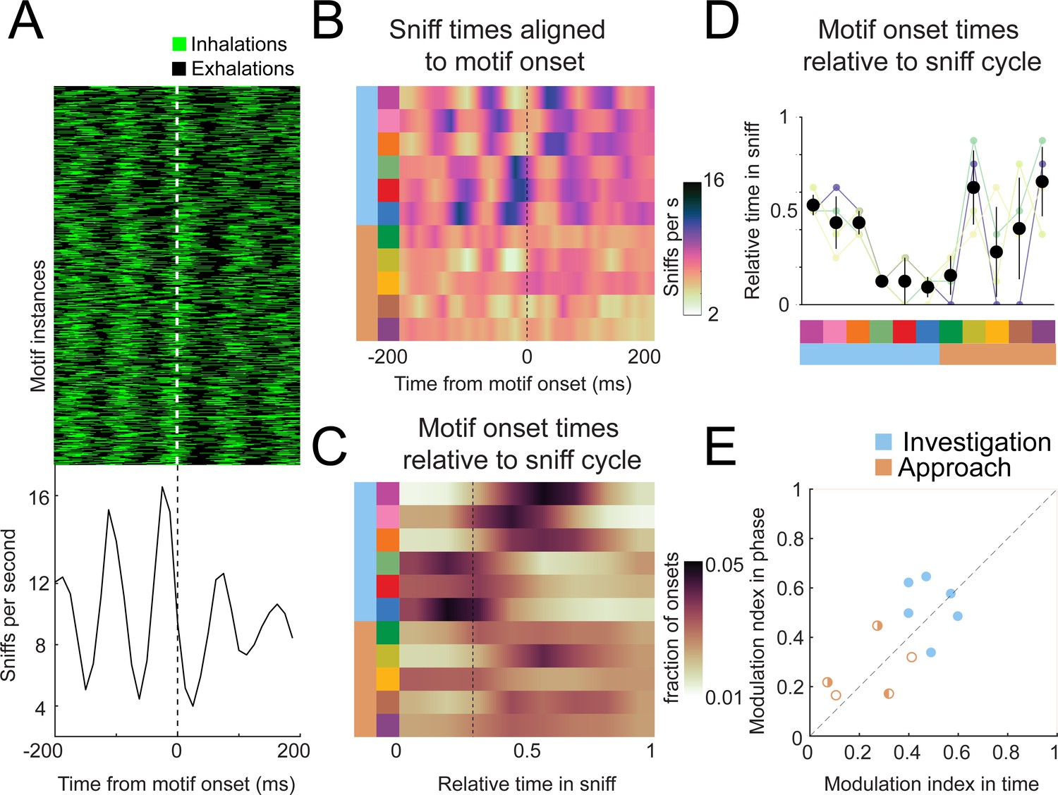
Motif onsets synchronize to the sniff cycle.
(A) Alignment of the sniff signal to an example motif. Top: color scheme shows sniff cycles aligned to the onsets of motif 6 (blue). Motif instances are in chronological order. Green: inhalation; black: rest of sniff. Bottom: peristimulus time histogram of inhalation times aligned to the onset of motif 6. (B) Alignment of sniff signal to onset times of all motifs across mice (n = 4). Motifs categorized into two types we call investigation (light blue) and approach (orange). Colormap represents the grand means for peristimulus time histograms of inhalation times aligned to the onset of motifs. (C) Alignment of motif onset times in sniff phase. Colormap represents peristimulus time histograms of motif onsets (bin width = 12.5 ms) times aligned to inhalation onset, with all sniff durations normalized to 1. Dotted line shows the mean phase of the end of inhalation. (D) Motif alignment to sniff phase is consistent across mice. Thin lines represent individual mice, black points are means, and whiskers are ±1 standard deviation (n = 4 mice). (E) Investigation motifs are more synchronized to the sniff cycle than approach motifs. Dots represent the modulation index in time on the x-coordinates and in phase on the y-coordinates. Filled dots represent motifs that are significantly modulated in both time and phase (p<0.01, permutation test). Half-filled dots represent motifs that are significantly modulated in time (left half filled) or phase (right half filled).
Figure 8—figure supplement 1
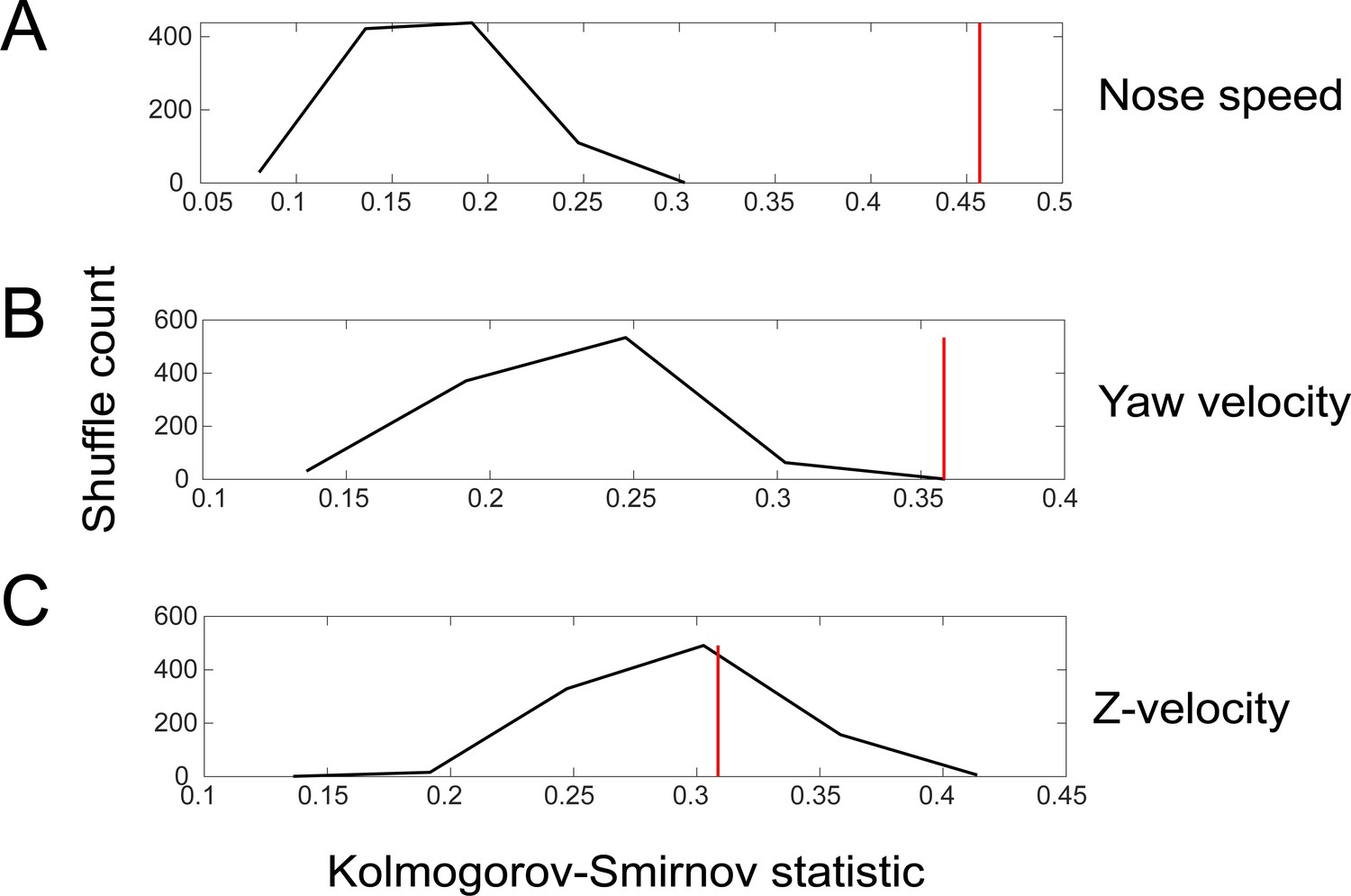
Shuffle test for the difference in sniff synchronization between investigation and approach motifs for movement parameters.
We quantified the difference by calculating the Kolmogorov–Smirnov statistic for the comparison between the sniff-triggered averages in the two states, first for real data, and then for 1000 iterations of trial-shuffled data. Red shows the value for the real data, while the black histogram plots the distribution of Kolmogorov–Smirnov statistic for the 1000 iterations. (A) Nose speed. (B) Yaw velocity. (C) Z-velocity.
Figure 8—figure supplement 2
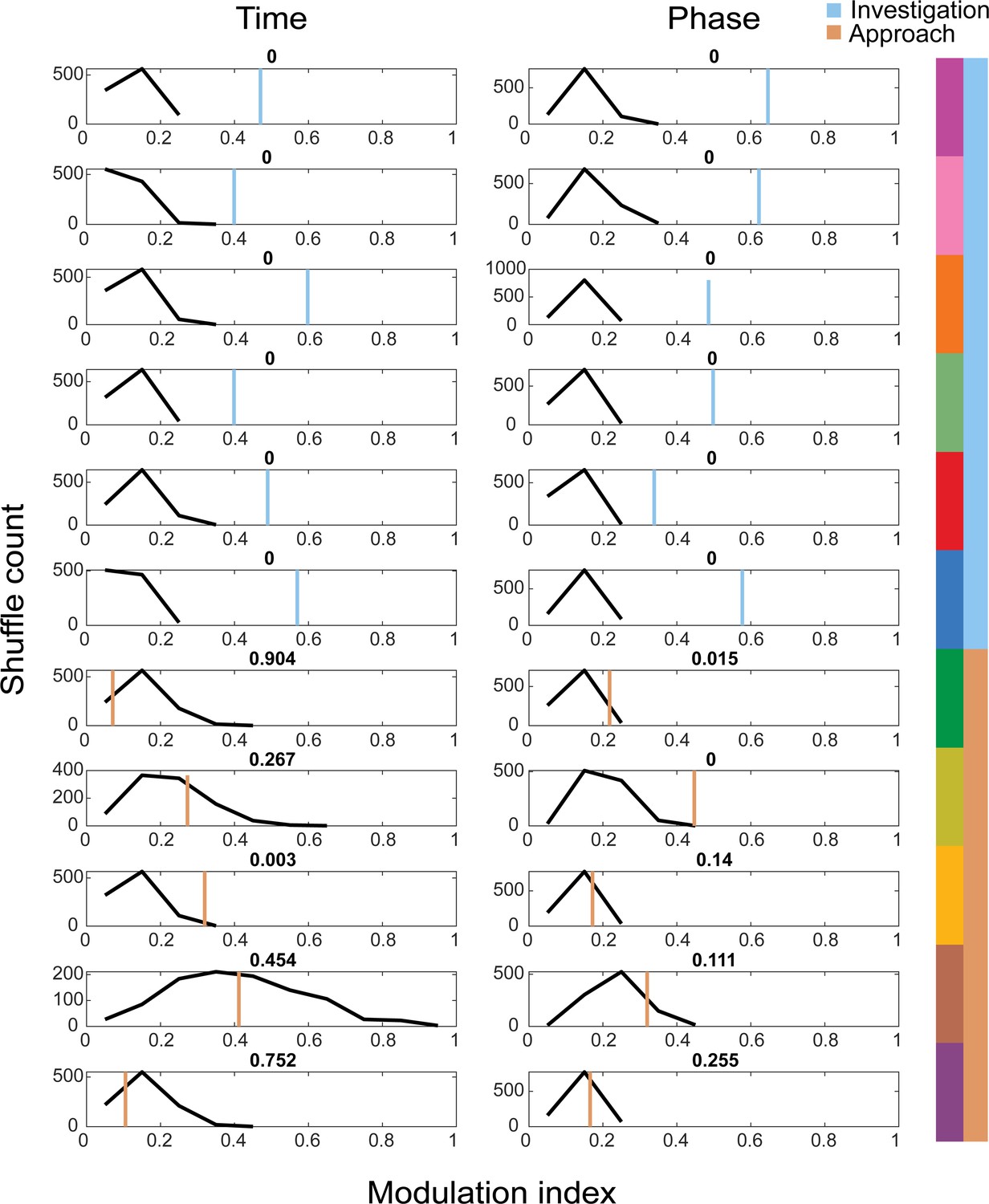
Shuffle test for sniff synchronization of motif onset for investigation and approach motifs.
We calculated a modulation index for each motif's across-mouse mean histogram (n = 4) and calculated the same for 1000 trial-shuffled across-mouse mean histograms. Blue and orange lines give the value from the real data, while the black histogram shows the distribution of MI across shuffle iterations.
Figure 9 with 1 supplement
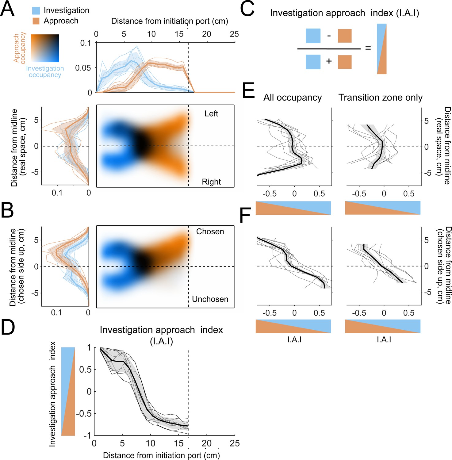
The allocentric spatial distribution of investigation and approach occupancy.
(A) Colormaps show two-dimensional histograms of the occupancy density (1 cm² bins, n = 9 mice) with investigation density in blue, approach density in orange, and overlap shown by darker coloring (key in top-left corner). Histograms around the colormaps show the state occupancy projected onto the longitudinal (top) and lateral (left) axes of the arena. (B) Occupancy distributions after the right-choice trials are flipped upward so that the chosen side is always facing up in the diagram. (C) Relative usage is quantified with an investigation approach index (I.A.I.), defined as the difference between investigation and approach occupancy divided by their sum. Blue and orange triangles are visual aids that represent the I.A.I. (D) Relative occupancy density of investigation and approach (I.A.I.), plotted along the longitudinal axis of the arena from the initiation port to the decision line. We define the region between 5 cm and 10 cm as a ‘transition zone’, in which most transitions between investigation and approach take place. Thin lines are individual mice (n = 9), thick line and shaded region are mean ± s.e.m. (E) I.A.I. plotted along the lateral axis in real space (i.e., left-right orientation) for all occupancy throughout the arena (left) and for the transition zone only (right). Thin lines are individual mice (n = 9), thick line and shaded region are mean ± s.e.m. (F) Same as (E), but after the lateral axis has been reoriented so that the chosen side is always up.
Figure 9—figure supplement 1
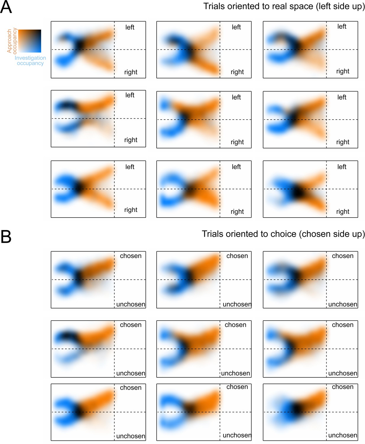
The allocentric spatial distribution of investigation and approach occupancy for individual mice.
(A) Colormaps show two-dimensional histograms of the occupancy density (1 cm² bins, n = 9 mice), with investigation density in blue, approach density in orange, and overlap shown by darker coloring (key in top-left corner). Each map corresponds to a single mouse. Trials are oriented with respect to real space, such that the left side of the arena faces up in the figure. (B) Same as (A), except that trials are reoriented so that the chosen side always faces up in the figure.
Figure 10 with 1 supplement

Occupancy maps indicate an advantage for investigation of both sides.
(A) Colormaps show two-dimensional histograms of the occupancy density (1 cm² bins, n = 9 mice) with investigation density in blue, approach density in orange, and overlap shown by darker coloring (key in top-left corner). Histograms around the colormaps show the state density projected onto the longitudinal (top) and lateral (left) axes of the arena. Left: correct trials. Right: incorrect trials. (B) Investigation approach index (I.A.I.) for correct (purple) and incorrect (green) trials. Thick lines and shaded region are mean ± s.e.m., thin lines are individual mice. (C) Difference in I.A.I. between correct and incorrect trials along the longitudinal axis (2.5 cm bins, n = 9). Thick line is the across-mouse mean difference, thin gray lines are 1000 permutations in which correct and incorrect trial labels were scrambled. (D) Investigation occupancy along the lateral axis, within the transition zone (5–10 cm longitudinal) for correct and incorrect trials. Thick lines and shaded region are mean ± s.e.m., thin lines are individual mice. (E) Approach occupancy along the lateral axis, within the transition zone (5–10 cm longitudinal) for correct and incorrect trials. Thick lines and shaded region are mean ± s.e.m., thin lines are individual mice. (F) I.A.I. along the lateral axis, within the transition zone (5–10 cm longitudinal) for correct and incorrect trials. Thick lines and shaded region are mean ± s.e.m., thin lines are individual mice. (G) Difference in investigation occupancy between correct and incorrect trials along the lateral axis, within the transition zone. Thick blue line is the across-mouse mean difference, thin blue lines are 1000 permutations in which correct and incorrect trial labels were scrambled. (H) Difference in approach occupancy between correct and incorrect trials. Thick orange line is the across-mouse mean difference, thin orange lines are 1000 permutations in which correct and incorrect trial labels were scrambled. (I) Difference in I.A.I. between correct and incorrect trials. Thick orange line is the across-mouse mean difference, thin orange lines are 1000 permutations in which correct and incorrect trial labels were scrambled.
Figure 10—figure supplement 1
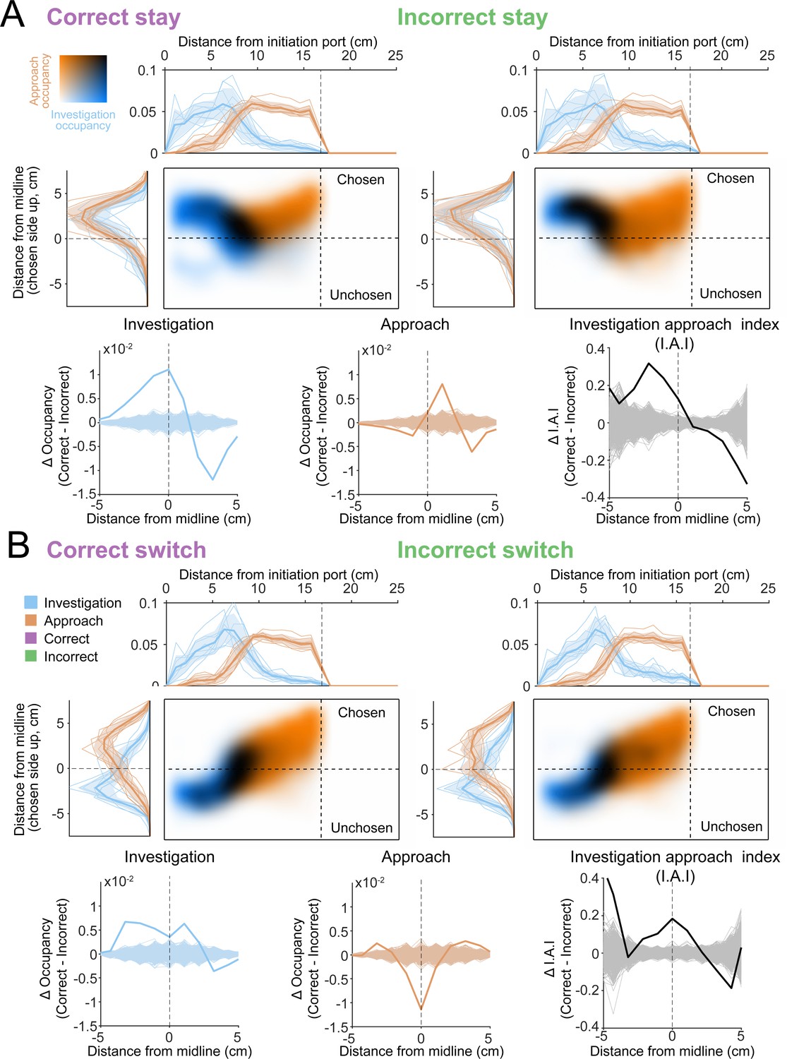
Occupancy maps indicate an advantage for investigation of both sides for both stay trials and switch trials.
(A) Occupancy map analysis for ‘stay’ trials (trials where the mouse chooses the side it first turned to, analyses as in Figure 10). (B) Occupancy map analysis for ‘switch’ trials (trials where the mouse chooses the opposite side from its first turn).
Videos
Video 1
Odor gradients are temporally dynamic and noisy.
Colormaps represent the time course of odor concentration for pseudo-trials assembled from individual trials at each sampling location.
Video 2
Example trials with sniffing.
Three dots on the mouse represent the coordinates of front of snout, back of head, and center of mass extracted using Deeplabcut. Sniffing is indicated by color (blue = inhalation, pink = exhalation) and sound (higher tone = inhalation, lower tone = exhalation). Video frame rate is slowed by 4×.
Video 3
Movement trajectories for individual sniffs.
Each video snippet corresponds to one sniff, where the frames are translated so that the back of the head is centered, and rotated so that the head angle is vertical, in the first frame of each sniff. Blue = inhalation, pink = exhalation. Video frame rate is slowed by 10×.
Video 4
Example trials with motif sequences.
Three dots on the mouse represent the coordinates of front of snout, back of head, and center of mass extracted using Deeplabcut. Dots and lines are colored according to the motif to which that frame was assigned by the auto-regressive hidden Markov model. Video frame rate is slowed by 8×.
Video 5
Moving occupancy histograms for motifs show their average movement dynamics.
We aligned every instance of a given motif such that that instance’s frames were translated to position the center of mass in frame 1 at consistent location in the image and rotated so that the body axis points upward in frame 1. Colormap represents regions of high occupancy with brighter, warmer colors, and lower occupancies with darker, colder colors. Video frame rate is slowed by 8×.
Video 6
Moving wireframes for motifs show the variability of movement dynamics for a given motif.
Wireframes consist of two lines connecting coordinates of front of snout, back of head, and center of mass extracted using Deeplabcut. Each wireframe represents a single instance of every motif. We aligned frames as in Video 5. Lines are colored arbitrarily to facilitate visualization of individual wireframes. Video frame rate is slowed by 8×.
Video 7
Example trials with investigation/approach overlaid.
Three dots on the mouse represent the coordinates of front of snout, back of head, and center of mass extracted using Deeplabcut. Dots and lines are colored according to whether that frame was assigned by the auto-regressive hidden Markov model to an investigation motif or an approach motif. Sniffing is indicated by sound (higher tone = inhalation, lower tone = exhalation). Video frame rate is slowed by 8×.
Video 8
Movement trajectories for individual sniffs separated into investigation and approach.
Each video snippet corresponds to one sniff, where the frames are translated so that the back of the head is centered and rotated so that the head angle is vertical, in the first frame of each sniff. Blue = inhalation, pink = exhalation. Video frame rate is slowed by 10×.
Tables
Key resources table
| Reagent type (species) or resource | Designation | Source or reference | Identifiers | Additional information |
|---|---|---|---|---|
| Software, algorithm | Bonsai | Open Ephys Lopes et al., 2015 | Visual reactive programming | |
| Software, algorithm | Deeplabcut | The Mathis Lab of Adaptive Motor Control Nath et al., 2019 | Animal pose estimation | |
| Software, algorithm | Pyhsmm | Matthew Johnson,Johnson et al., 2013a and Johnson et al., 2013b | Bayesian inference in HSMMs and HMMs |
Additional files
Download links
A two-part list of links to download the article, or parts of the article, in various formats.
Downloads (link to download the article as PDF)
Open citations (links to open the citations from this article in various online reference manager services)
Cite this article (links to download the citations from this article in formats compatible with various reference manager tools)
Sniff-synchronized, gradient-guided olfactory search by freely moving mice
eLife 10:e58523.
https://doi.org/10.7554/eLife.58523


