Binding mechanism of the matrix domain of HIV-1 gag on lipid membranes
- Department of Chemistry, Chicago Center for Theoretical Chemistry, Institute for Biophysical Dynamics, and The James Franck Institute, The University of Chicago, United States
Figures
Figure 1

Matrix (MA) domain of HIV-1 Gag (residues 1–120) with key regions labeled: H1, H2, H3, H4, and H5 are helices numbered in order of appearance in the protein sequence; Myr is the lipidated tail of MA attached covalently to the N-terminus of the protein (shown in red); the lid is a small helical region that locks Myr inside the protein hydrophobic pocket; the HBR is a coiled region rich in LYS and ARG residues that is the main contributor to electrostatic interactions with the membrane.
Figure 2 with 6 supplements
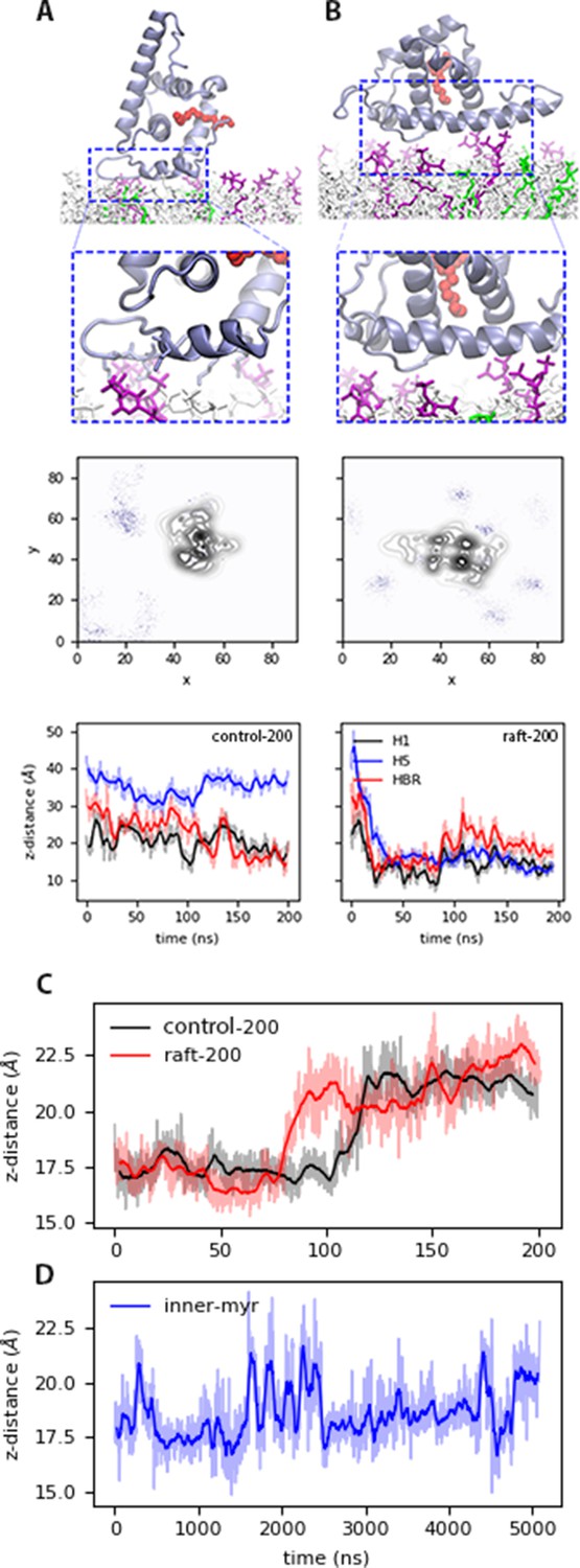
Bound states of MA with model membranes.
(A) In the open state with the control200 model, and (B) the blocked state with the raft200 model. Top: snapshots of the bound conformations, PIP2 lipids are shown in purple and DOPS in green. Center: PIP2 lipid density at the end of the 200-ns trajectories. Bottom: distance between protein sections and the phosphate region of the lipids in the binding leaflet for each conformation. Time series of the distance between H1 and Lid of MA, that is the mouth of the protein for the (C) control200 and raft200 systems with an open-bound and a blocked-bound MA, respectively. (D) H1-Lid distance for the innermyr model trajectory. Moving average for these plots is shown in bold lines every 5 ns for the 200-ns trajectories, and every 50 ns for the microsecond trajectory in bold lines; the faded curves are the original dataset. The chemical structures of each lipid species in the membrane models is shown in Figure 2—figure supplement 1.
-
Figure 2—source code 1
Python script to generate the bottom density plot of panels A and B in Figure 2.
- https://cdn.elifesciences.org/articles/58621/elife-58621-fig2-code1-v2.zip
-
Figure 2—source data 1
Data to generate the bottom density plot of panels A in Figure 2.
- https://cdn.elifesciences.org/articles/58621/elife-58621-fig2-data1-v2.txt
-
Figure 2—source data 2
Data to generate the bottom density plot of panels B in Figure 2.
- https://cdn.elifesciences.org/articles/58621/elife-58621-fig2-data2-v2.txt
Figure 2—figure supplement 1

Chemical structures of the lipids used in the membrane models for this study.
The lipid tail saturation nomenclature is given for the sn2 – sn1 tails below each name, and the full names for each species: DOPC: 1,2-dioleoyl-sn-glycero-3-phosphocholine. DOPS: 1,2-dioleoyl-sn-glycero-3-phospho-L-serine. POPE: 1-palmitoyl-2-oleoyl-sn-glycero-3-phosphoethanolamine. BSM: N-octadecanoyl-D-erythro-sphingosylphosphorylcholine, a.k.a.(porcine) brain sphingomyelin. PIP2: 1,2-dioctanoyl-sn-glycero-3-phospho-(1’-myo-inositol-4’,5’-biphosphate).
Figure 2—figure supplement 2
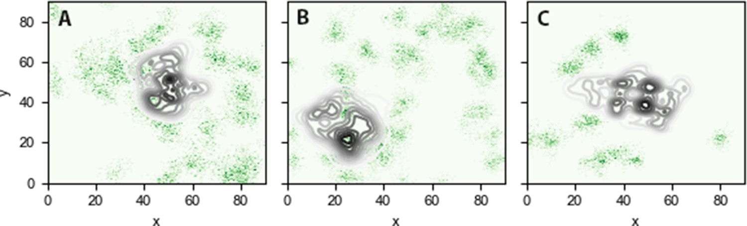
Lipid densities of DOPS lipids in the binding leaflets of the symmetric membrane models at the end of 200 ns of equilibration.
(A) control200, (B) inner200, and (C) raft200. Densities computed over last 50 ns of trajectory.
-
Figure 2—figure supplement 2—source code 1
Python script to generate panels A, B, and C in the corresponding figure.
- https://cdn.elifesciences.org/articles/58621/elife-58621-fig2-figsupp2-code1-v2.zip
-
Figure 2—figure supplement 2—source data 1
XY coordinates to plot the lipid density for DOPS in the binding leaflet.
- https://cdn.elifesciences.org/articles/58621/elife-58621-fig2-figsupp2-data1-v2.txt
Figure 2—figure supplement 3
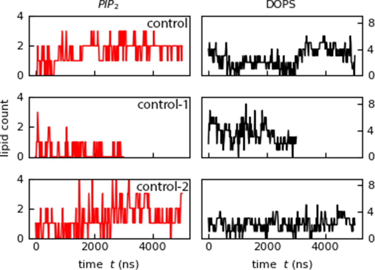
Protein-lipid contacts for the control models with pre-inserted Myr (controlpre, control-1pre, control-2pre).
Figure 2—figure supplement 4
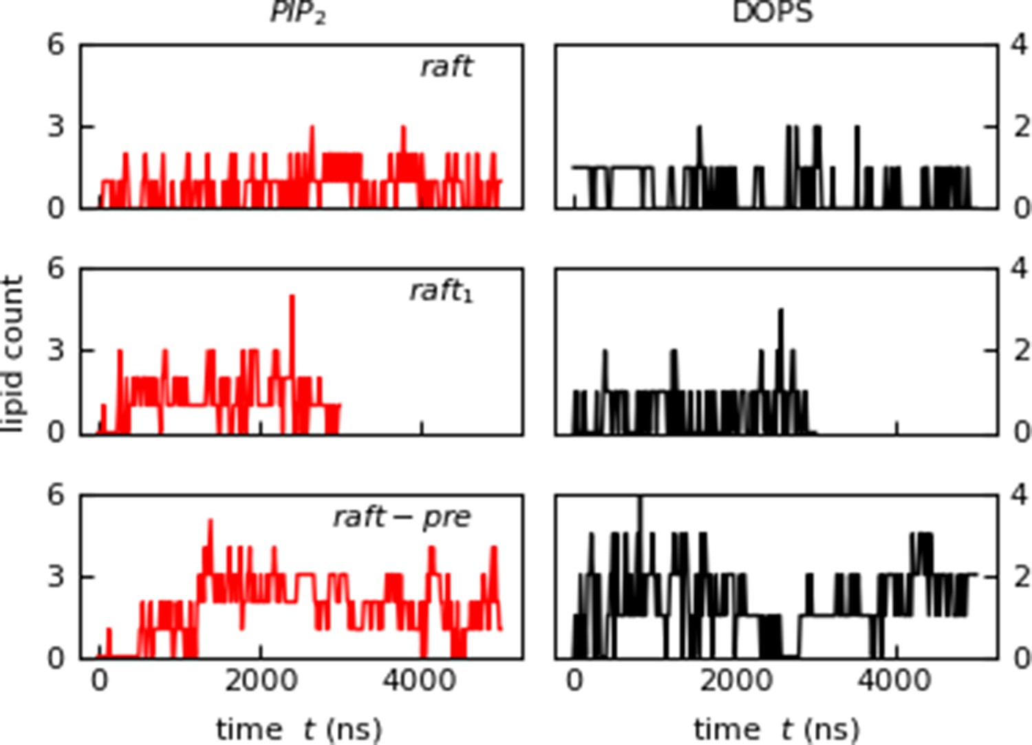
Protein-lipid contacts for the raft, raft-1 and raftpre trajectories.
Figure 2—figure supplement 5
Snapshots of the protein-membrane interactions for the raftpre model trajectory (pre-inserted Myr).
Figure 2—figure supplement 6

Timeseries for the distance between H1, H5, and the HBR and the bilayer center for the raftpre system.
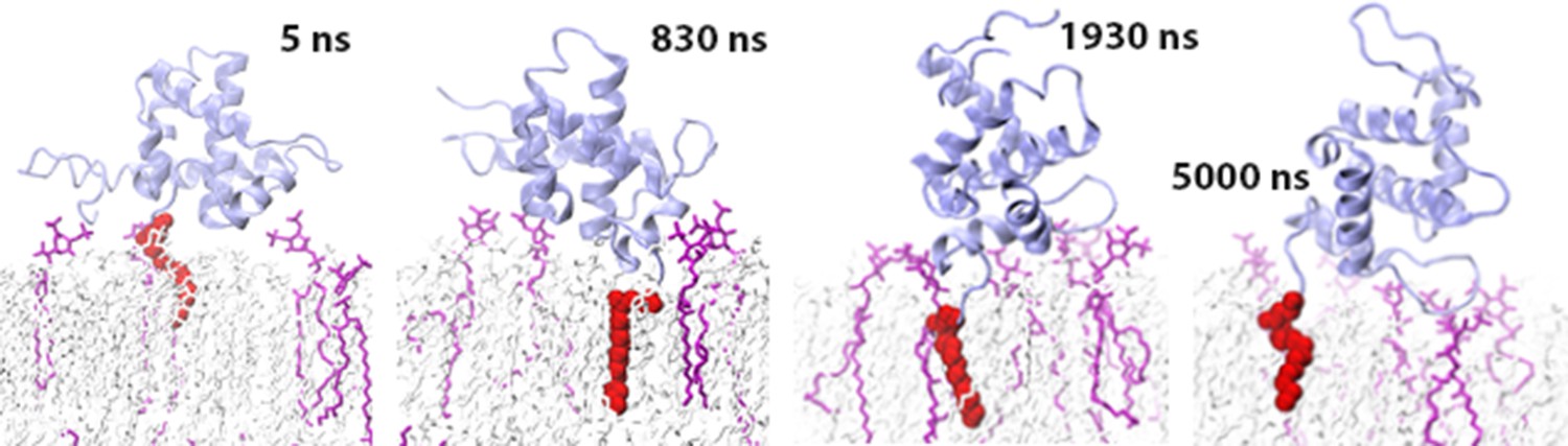
Figure 3 with 1 supplement
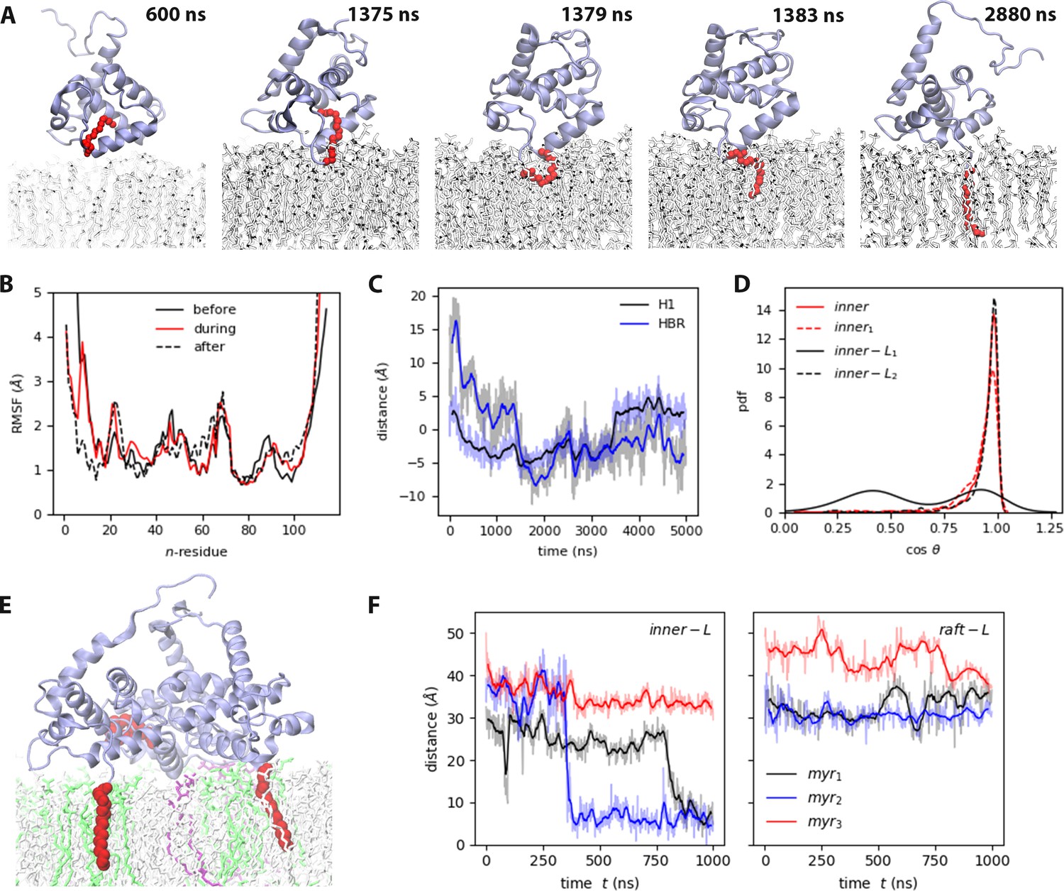
Myr insertion mechanism.
(A) Trajectory snapshots from the inner trajectory, see also Video 2. (A) Myristate insertion mechanism (from the inner trajectory), see also Video 2. (B) RMSF of MA before, during, and after Myr insertion, at least 50 ns of the respective sections in the inner trajectory were used for this analysis. (C) Self-distance of H1 and HBR during Myr insertion (refer to Table S3 in Supplementary file 1 for the definition of self-distance). (D) Probability distribution of the angle between Myr and the bilayer normal for the MA units that exhibit Myr insertion (see also Figure 3—figure supplement 1). (E) Snapshot of the side view of inner-Ltrimer at the end of the simulation, PIP2 lipids are shown in purple, DOPS lipids in green. (F) Time series of Myr insertion in the first and second MA units in the inner-Ltrimer simulation, the distance was computed between the last carbon in the lipid tail (C14) and the bilayer center. All the time series show the blocked moving averaged in solid color and the raw data faded.
Figure 3—figure supplement 1
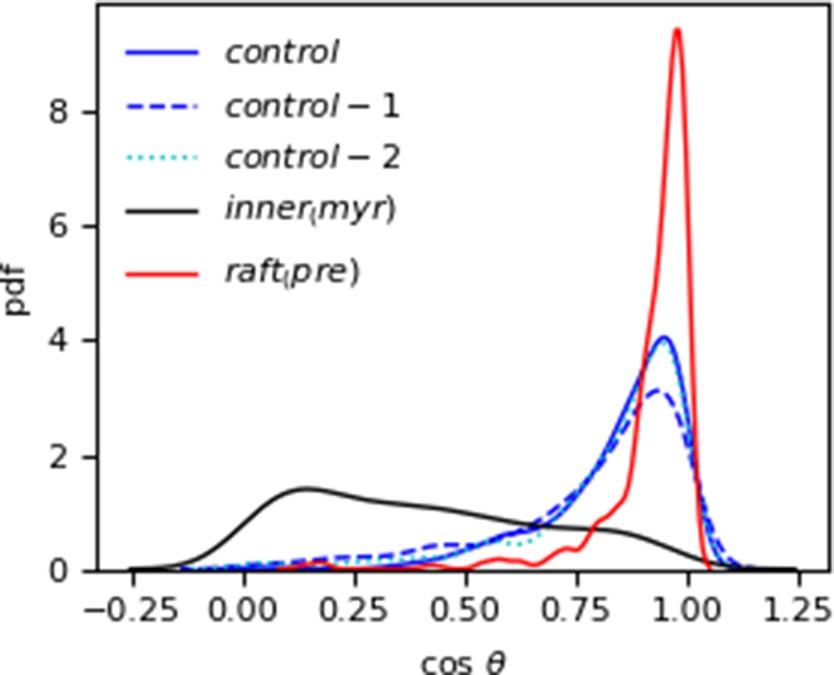
Probability distribution of the cosine of the angle between Myr and the bilayer normal (z-axis) in the systems starting from a pre-inserted Myr configuration.
The innermyr system is also included as reference for a lipid tail that returned to the protein hydrophobic cavity and is essentially parallel to the membrane surface (black curve).
Figure 4
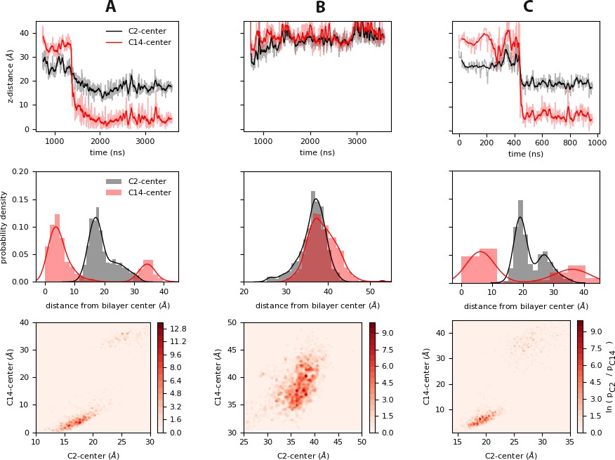
Relative motions of the Myr tail during insertion.
Top: Time series of insertion for the first and last carbons in the Myr tail, C2 and C14; the distance was computed between the center of mass of the respective carbon and the bilayer center as estimated from the average distance between the phosphate regions of the lipids in each leaflet. The faded regions show the raw data of this metric, and the bolded regions show the corresponding blocked moving average. Center: Probability density of the same distances as estimated from the normalized histograms of each time series. Bottom: Heat maps of the probabilities of the C2 and C14 atoms of Myr as estimated from the histogrammed data. The systems shown are: (A) inner, (B) innermyr, and (C) inner-Ltrimer (MA2 unit).
-
Figure 4—source code 1
Python script to generate panel A; (top).
Timeseries for the distance between C2 and C14 carbons of Myr and the center of the bilayer, (center) probability density of the same carbons with respect to their position in the z-axis, (bottom) heatmap of these probabilities.
- https://cdn.elifesciences.org/articles/58621/elife-58621-fig4-code1-v2.zip
-
Figure 4—source code 2
Python script to generate panel B; (top).
Timeseries for the distance between C2 and C14 carbons of Myr and the center of the bilayer, (center) probability density of the same carbons with respect to their position in the z-axis, (bottom) heatmap of these probabilities.
- https://cdn.elifesciences.org/articles/58621/elife-58621-fig4-code2-v2.zip
-
Figure 4—source code 3
Python script to generate panel C; (top).
Timeseries for the distance between C2 and C14 carbons of Myr and the center of the bilayer, (center) probability density of the same carbons with respect to their position in the z-axis, (bottom) heatmap of these probabilities.
- https://cdn.elifesciences.org/articles/58621/elife-58621-fig4-code3-v2.zip
-
Figure 4—source data 1
Data to generate panel A.
(Top) Timeseries for the distance between C2 and C14 carbons of Myr and the center of the bilayer, (Center) probability density of the same carbons with respect to their position in the z-axis, (Bottom) heatmap of these probabilities.
- https://cdn.elifesciences.org/articles/58621/elife-58621-fig4-data1-v2.txt
-
Figure 4—source data 2
Data to generate panel B.
(Top) Timeseries for the distance between C2 and C14 carbons of Myr and the center of the bilayer, (Center) probability density of the same carbons with respect to their position in the z-axis, (Bottom) heatmap of these probabilities.
- https://cdn.elifesciences.org/articles/58621/elife-58621-fig4-data2-v2.txt
-
Figure 4—source data 3
Data to generate panel C.
(Top) Timeseries for the distance between C2 and C14 carbons of Myr and the center of the bilayer, (Center) probability density of the same carbons with respect to their position in the z-axis, (Bottom) heatmap of these probabilities.
- https://cdn.elifesciences.org/articles/58621/elife-58621-fig4-data3-v2.txt
Figure 5 with 2 supplements
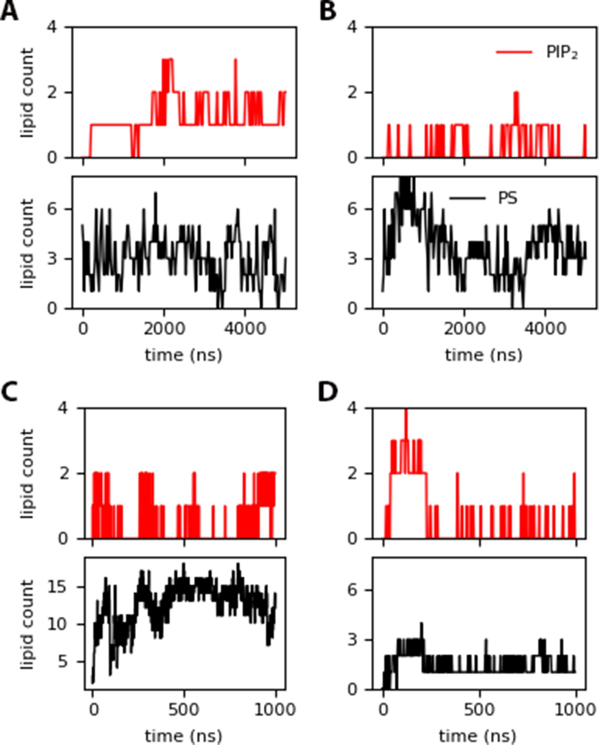
PIP2 and DOPS contacts within 10 of the protein for: (A) inner (insertion around 1380 ns), (B) innermyr, (C) inner-Ltrimer (with permanent Myr insertion after 400 ns), and (D) raft-Ltrimer (with no insertion).
Figure 5—figure supplement 1
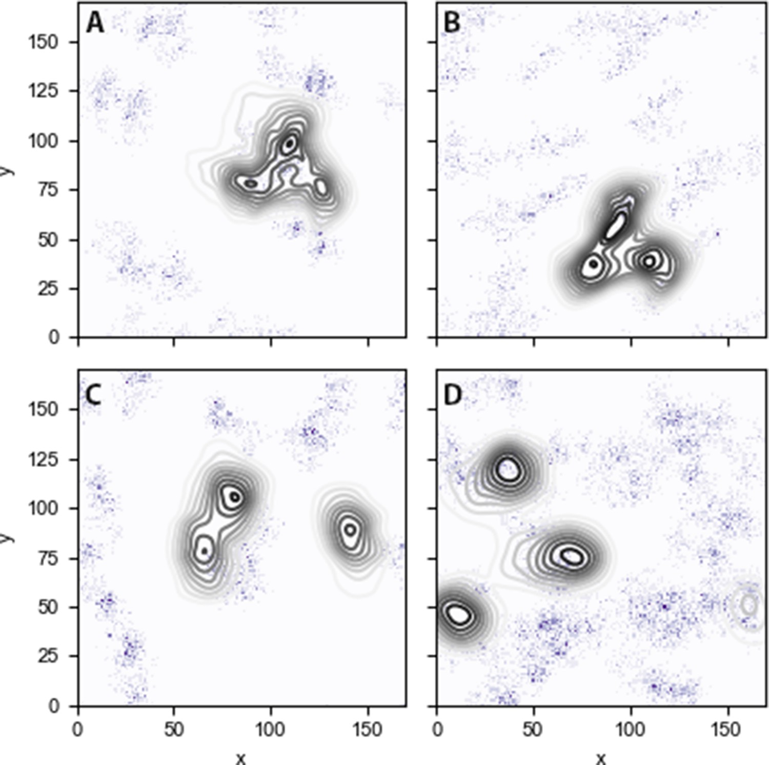
PIP2 lipid densities in the binding leaflet for the: (A) inner-Ltrimer (B) raft-Ltrimer, (C) inner-Lmono (D) raft-Lmono systems.
Data was computed over the last 200 ns of simulation.
-
Figure 5—figure supplement 1—source code 1
Python script to plot the lipid density for PIP2 in the binding leaflet for the (A) inner-Ltrimer (B) raft-Ltrimer, (C) inner-Lmono (D) raft-Lmono systems.
- https://cdn.elifesciences.org/articles/58621/elife-58621-fig5-figsupp1-code1-v2.zip
-
Figure 5—figure supplement 1—source data 1
XY coordinates to plot the lipid density for PIP2 in the binding leaflet for the (A) inner-Ltrimer (B) raft-Ltrimer, (C) inner-Lmono (D) raft-Lmono systems.
- https://cdn.elifesciences.org/articles/58621/elife-58621-fig5-figsupp1-data1-v2.zip
Figure 5—figure supplement 2

Lipid densities for sphingomyelin (top) and cholesterol (bottom) lipids in the binding and opposite leaflets, for the inner-Ltrimer trajectory.
Data collected over the last 200 ns of simulation.
-
Figure 5—figure supplement 2—source code 1
Python script to plot the lipid density for sphingomyelin and cholesterol in the binding and opposite leaflet, respectively.
- https://cdn.elifesciences.org/articles/58621/elife-58621-fig5-figsupp2-code1-v2.zip
-
Figure 5—figure supplement 2—source data 1
XY coordinates to plot the lipid density for sphingomyelin and cholesterol in the binding and opposite leaflet.
- https://cdn.elifesciences.org/articles/58621/elife-58621-fig5-figsupp2-data1-v2.zip
Figure 6
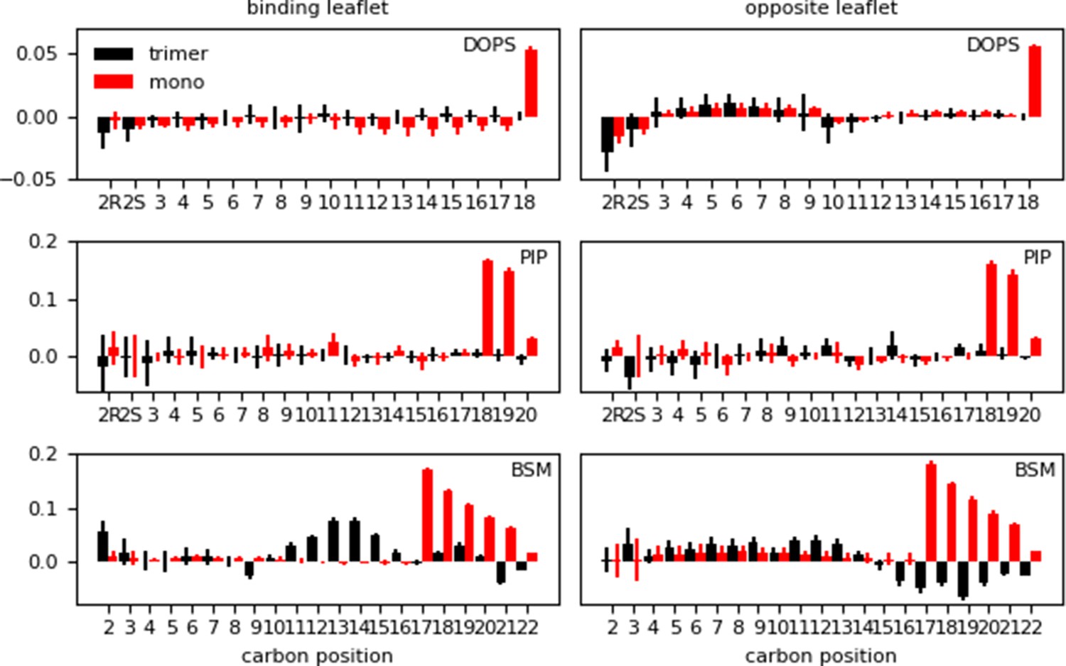
Difference in lipid order parameter (SCD) between the protein-membrane and membrane-only systems per leaflet for the inner (‘mono’) and inner-Ltrimer (‘trimer’) systems after Myr insertion.
A positive value indicates the presence of the protein with inserted Myr increases the order in the bilayer, whereas a negative value corresponds to a decrease in order with respect to the membrane-only system.
Figure 7 with 1 supplement
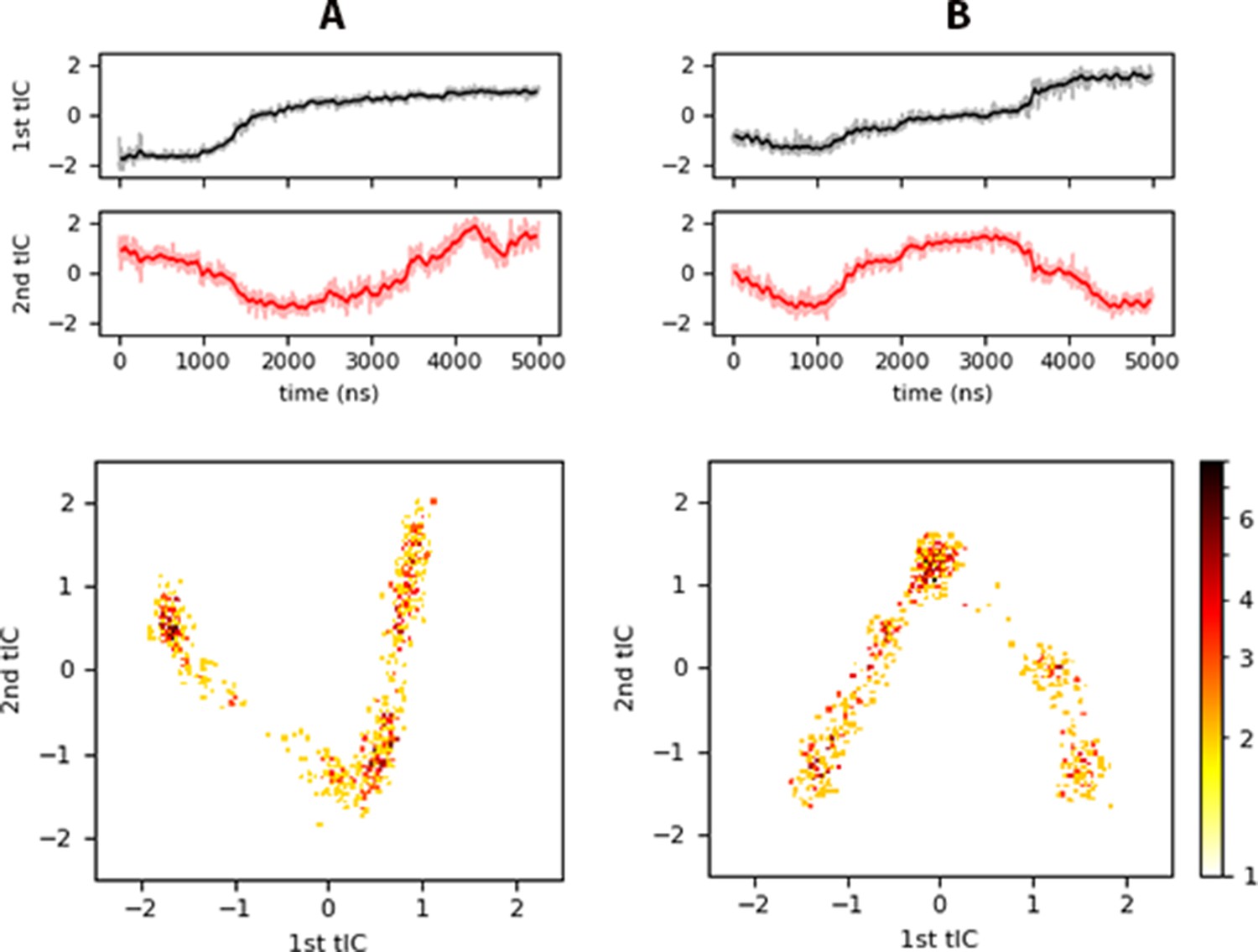
tICA results for (A) inner, and (B) innermyr.
Top panels show the projection of each trajectory onto the slowest independent components identified, and the bottom panels a heat map of histograms of the projected trajectory onto the respective tIC (logarithmic scale). Similar plots are shown in Figure 7—figure supplement 1 for the controlpre, raft, and raftpre systems.
-
Figure 7—source code 1
Python script to generate panels A and B of Figure 7 as well as A, B, and C of Figure 7—figure supplement 1; timeseries of the trajectory projected onto the first and second tIC components.
- https://cdn.elifesciences.org/articles/58621/elife-58621-fig7-code1-v2.zip
-
Figure 7—source data 1
Data to generate panel A of Figure 7; timeseries of the trajectory projected onto the first and second tIC components.
- https://cdn.elifesciences.org/articles/58621/elife-58621-fig7-data1-v2.txt
-
Figure 7—source data 2
Data to generate panel B of Figure 7; timeseries of the trajectory projected onto the first and second tIC components.
- https://cdn.elifesciences.org/articles/58621/elife-58621-fig7-data2-v2.txt
Figure 7—figure supplement 1

tICA results for (A) controlpre, (B) raft, and (C) raftpre trajectories.
Top panels show the projection of each trajectory onto the slowest independent components identified, and the bottom panels are heat-maps in logarithmic scale estimated from histograms of the projected trajectory onto the two slowest tICs.
-
Figure 7—figure supplement 1—source data 1
Data for panel A of Figure 7—figure supplement 1; timeseries of the trajectory projected onto the first and second tIC components.
- https://cdn.elifesciences.org/articles/58621/elife-58621-fig7-figsupp1-data1-v2.txt
-
Figure 7—figure supplement 1—source data 2
Data for panel B of Figure 7—figure supplement 1; timeseries of the trajectory projected onto the first and second tIC components.
- https://cdn.elifesciences.org/articles/58621/elife-58621-fig7-figsupp1-data2-v2.txt
-
Figure 7—figure supplement 1—source data 3
Data for panel C of Figure 7—figure supplement 1; timeseries of the trajectory projected onto the first and second tIC components.
- https://cdn.elifesciences.org/articles/58621/elife-58621-fig7-figsupp1-data3-v2.txt
Videos
Video 1
MA binding in the open conformation.
The protein binds within the first 50 ns of simulation trajectory; electrostatic interactions with charged lipid headgroups are strong enough to keep the protein bound to the membrane surface, and Myr is free to survey the membrane surface.
Video 2
‘Myr insertion into a model membrane.
Exposure of Myr, the lipid tail of MA, occurs within the first 200 ns of trajectory. The tail can survey the membrane surface and even extend towards the water before permanently inserting into the bilayer.
Tables
Table 1
Simulation components for the membrane models used in this study.
Chemical structures of each lipid species are shown in Figure 2—figure supplement 1.
| Model | Lipid species | Lipid mol fract. | Charge density (e-/nm2) | Unsat. degree | # Waters (small) | Ions | # Waters (large) | Ions |
|---|---|---|---|---|---|---|---|---|
| Control APL* 66.9 +/- 0.84 | DOPC DOPS PIP2‡ | 0.80 0.15 0.05 | −0.25 | 0.98 | 23442 78.1 H-num† | 211 K 112 Cl | - | - |
| Inner APL 47.8 +/- 0.40 | Chol DOPC DOPS POPE BSM PIP2 | 0.30 0.17 0.17 0.25 0.08 0.02 | −0.26 | 0.52 | 16009 (53.4) H-num | 154 K 81 Cl | 103544 (86.3) H-num | 295 K |
| Raft APL 47.1 +/- 0.40 | Chol DOPC DOPS BSM PIP2 | 0.28 0.30 0.06 0.30 0.06 | −0.32 | 0.54 | 15744 (52.6) H-num | 170 K 83 Cl | 100034 (83.4) H-num | 351 K |
-
*Area per lipid (Å2/lipid).
†ydration number (# waters/lipid).
-
‡SAPI25 in CHARMM36m topology (18:0 - 20:4).
Table 2
Summary of insertion events for the systems that exhibit Myr insertion.
The angle reported in the last column is that between the Myr tail and the bilayer normal, taken as the positive z-axis. The standard error is reported along with the angles.
| System | Sim time (μs) | Bound conf. | Bound leaflet | insertion (ns) | Myr angle (o) |
|---|---|---|---|---|---|
| Inner | 5 | Open | Bottom | 1380 ± 2 | 25.4 ± 2.3 |
| Inner-1 | 1.6 | Open | Bottom | 78 ± 1 | 8.2 ± 1.4 |
| Inner-Ltrimer | 1 | Open | Top | MA1: 350 ± 4 MA2: 780 ± 2 MA3: none | MA1: 37.8 ± 5.4 MA2: 18.1 ± 3.2 MA3: N/A |
Additional files
-
Supplementary file 1
Tables S1-S3 cited and discussed in this work.
These list detailed information about all the systems of study, and thorough description of the quantitative analysis performed in the collected simulation data.
- https://cdn.elifesciences.org/articles/58621/elife-58621-supp1-v2.docx
-
Transparent reporting form
- https://cdn.elifesciences.org/articles/58621/elife-58621-transrepform-v2.pdf
Download links
A two-part list of links to download the article, or parts of the article, in various formats.
Downloads (link to download the article as PDF)
Open citations (links to open the citations from this article in various online reference manager services)
Cite this article (links to download the citations from this article in formats compatible with various reference manager tools)
Binding mechanism of the matrix domain of HIV-1 gag on lipid membranes
eLife 9:e58621.
https://doi.org/10.7554/eLife.58621


