Extended field-of-view ultrathin microendoscopes for high-resolution two-photon imaging with minimal invasiveness
Figures
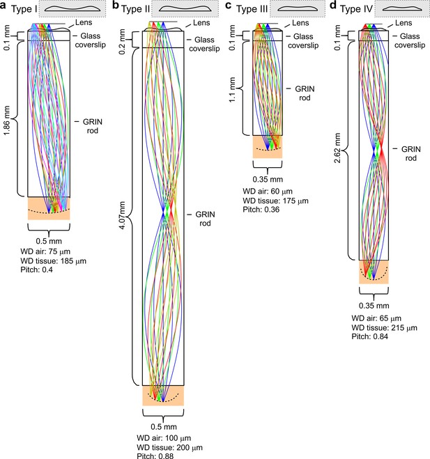
Optical design of eFOV-microendoscopes.
(a-d) Ray-trace simulations for the four different eFOV-microendoscopes (type I-IV). The insets show the profiles of corrective polymeric lenses used in the different eFOV-microendoscopes. For each eFOV-microendoscope, it is specified the thickness of the coverslip, the length, the diameter of the GRIN rod, the pitch of the GRIN rod, and the working distance, in air or in tissue, at which the simulated correction of aberrations was performed. See also Supplementary file 1 - Table 1.
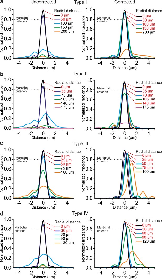
Corrective lenses improve the simulated optical performance of ultrathin microendoscopes.
(a) Simulated diffraction PSFs to assess the Strehl ratio of the designed microendoscope (type I microendoscopes) without the corrective lens (uncorrected, left) and with the corrective lens (corrected, right). PSFs are shown color-coded according to their radial distance from the optical axis. The black dotted line represents the diffraction-limited condition, which was set at 80% (Maréchal criterion). Distances written in red indicate the radial positions at which the maximal normalized irradiance of the corresponding PSF was >80%. (b–d) Same as in (a) for type II (b), type III (c), and type IV (d) microendoscopes. See also Figure 2—figure supplements 1–4.
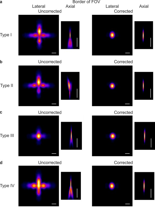
Aberration correction improves the simulated PSF in the peripheral portions of the FOV in eFOV-microendoscopes.
(a) Lateral and axial projection of a simulated PSF positioned at the border of the FOV with the uncorrected (left) and corrected (right) type I microendoscopes. Scale bars: 1 μm (lateral), 10 μm (axial). (b) Same as in (a) for type II microendoscopes. (c) Same as in (a) for type III microendoscopes. (d) Same as in (a) for type IV microendoscopes.
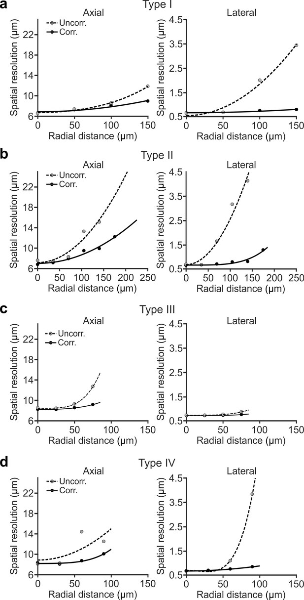
Simulated spatial resolution is improved in eFOV-microendoscopes.
(a) Simulated axial (left) and lateral (right) spatial resolution (see Materials and methods for definition) as a function of the radial distance from the center of the FOV for type I uncorrected (dashed line) and corrected (solid line) microendoscopes. Points represent simulated values, lines are quartic functions fitting the data. (b) Same as in (a) for type II microendoscopes. (c) Same as in (a) for type III microendoscopes. (d) Same as in (a) for type IV microendoscopes.
-
Figure 2—figure supplement 2—source data 1
Simulated values of the axial and lateral spatial resolution as a function of radial distance from the center of the FOV in uncorrected and corrected microendoscopes.
- https://cdn.elifesciences.org/articles/58882/elife-58882-fig2-figsupp2-data1-v3.xlsx
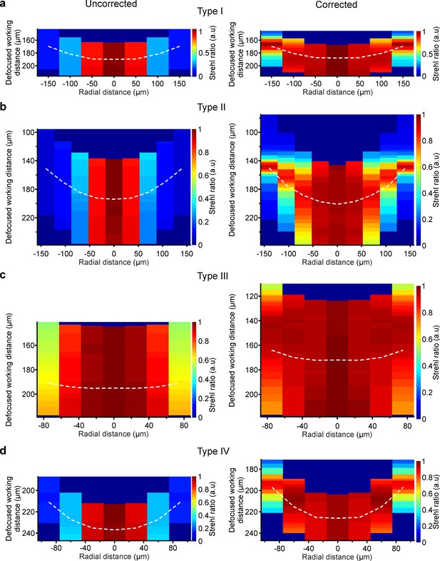
Corrective lenses enlarge the simulated volume that can be scanned during 3D imaging.
(a) Pseudocolor map showing the simulated Strehl ratio on a x,z section of the image space for type I uncorrected (left) and corrected (right) microendoscopes. The dashed white line represents a section of the imaging plane for which the corrective lens profile was optimized. In the case of uncorrected microendoscopes, it represents the section obtained with the same optical configuration, but without the corrective lens. (b) Same as in (a) for type II microendoscopes. (c) Same as in (a) for type III microendoscopes. (d) Same as in (a) for type IV microendoscopes.
-
Figure 2—figure supplement 3—source data 1
Simulated Strehl ratio as a function of the lateral and axial displacement for type I-IV uncorrected and corrected microendoscopes.
- https://cdn.elifesciences.org/articles/58882/elife-58882-fig2-figsupp3-data1-v3.xlsx
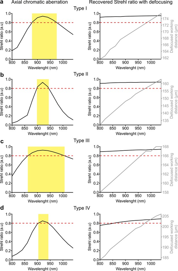
Chromatic aberrations in eFOV-microendoscopes.
(a) Left panel: Simulated Strehl ratio at the border of the FOV as a function of wavelength. The red dashed line represents the diffraction-limited condition, which was set at 80% (Maréchal criterion). The yellow area indicates the wavelength range that satisfies the Maréchal criterion. Right panel: highest simulated Strehl ratio (black line) at the border of the FOV and corresponding defocused working distance (gray line) as a function of wavelength. The red dashed line indicates the diffraction-limited condition as in the left panel. (b) Same as in (a) for type II microendoscopes. (c) Same as in (a) for type III microendoscopes. (d) Same as in (a) for type IV microendoscopes.
-
Figure 2—figure supplement 4—source data 1
Simulated Strehl ratio as a function of wavelength.
- https://cdn.elifesciences.org/articles/58882/elife-58882-fig2-figsupp4-data1-v3.xlsx
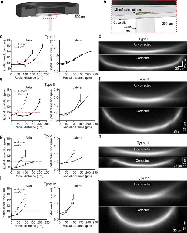
Optical characterization shows enlarged effective FOV in corrected ultrathin microendoscopes.
(a) Schematic of the eFOV-microendoscope mount for head implant. The GRIN rod is glued to one side of the glass coverslip, the microfabricated polymer lens to the other side of the coverslip. The coverslip is glued on a circular metal ring that facilitates fixation on the animal's skull. (b) Zoom in of the portion highlighted with the red dotted line in (a). (c) Axial (left) and lateral (right) spatial resolution (see Materials and methods for definition) evaluated using subresolved fluorescent beads (diameter: 100 nm) as a function of the radial distance from the center of the FOV for type I uncorrected (dashed line) and corrected (solid line) microendoscopes. Points represent values obtained by averaging at least eight measurements from three different probes (see Supplementary file 1 - Table 1), while error bar represents standard deviation (sd). Lines are quartic functions fitting the data. The red dashed line indicates a threshold value (10 µm) to define the limit of the effective FOV. (d) x,z projections (x, horizontal direction; z, vertical direction) of a z-stack of two-photon laser-scanning images of a subresolved fluorescent layer (thickness: 300 nm) obtained using a type I eFOV-microendoscope, without (uncorrected, top) and with (corrected, bottom) the microfabricated corrective lens. λexc = 920 nm. (e,f) Same as in (c,d) for type II eFOV-microendoscopes. (g,h) Same as in (c,d) for type III eFOV-microendoscopes. (i,j) Same as in (c,d) for type IV eFOV-microendoscopes. See also Figure 3—figure supplements 1–7 and Supplementary file 1 - Table 3.
-
Figure 3—source data 1
Experimental values of the axial and lateral spatial resolution as a function of radial distance from the center of the FOV in uncorrected and corrected microendoscopes.
- https://cdn.elifesciences.org/articles/58882/elife-58882-fig3-data1-v3.xlsx

Polymer lens fabrication using 3D micro-printing based on two-photon lithography.
(a) Schematic of the optical set-up for two-photon lithography. AOM, Acousto Optical Modulator; S, laser source; CCD, camera. (b) Scanning electron microscope image of a corrective polymer lens. (c) Blue dashed lines indicate the designed lens profile. Red lines represent the lens profile measured with a contact stylus surface profiler.
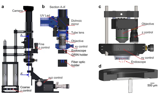
Set-ups for the assembly and characterization of eFOV-microendoscopes.
(a) Optomechanical stage used for microendoscope assembly. Red arrows indicate key components. The blue line indicates the plane used for the cross-section view shown at an expanded scale in b. (b) Section (A–A’) of the set-up shown in a. (c) Schematic of the optomechanical assembly used for microendoscopic imaging. (d) The eFOV-microendoscope assembly for implantation highlighted with the red dotted line in (c) is shown at an expanded scale.
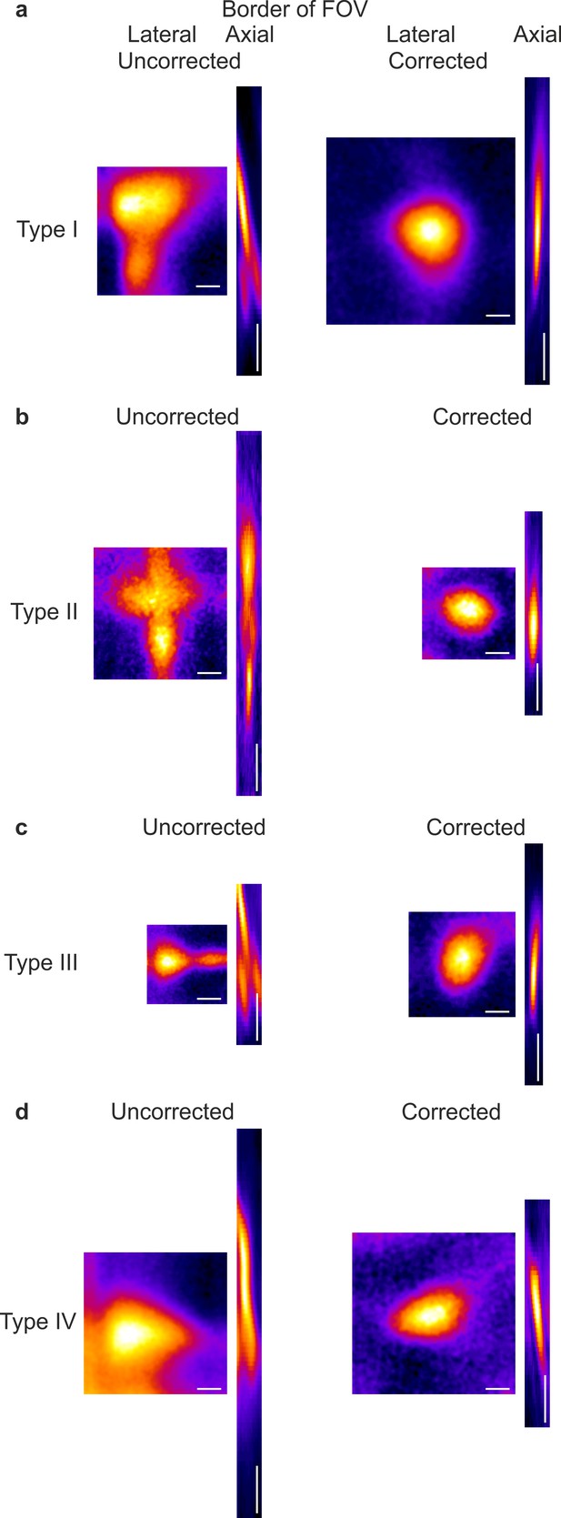
Aberration correction improves the PSF in the peripheral portions of the FOV in eFOV-microendoscopes.
(a) Lateral and axial projection of a z-stack of a subresolved fluorescent bead positioned at the border of the FOV and imaged with the uncorrected (left) and corrected (right) type I microendoscopes. Scale bars: 1 µm (lateral), 10 µm (axial). (b) Same as in (a) for type II microendoscopes. (c) Same as in (a) for type III microendoscopes. (d) Same as in (a) for type IV microendoscopes. Please note that the slight tilt of the axial PSF with respect to the optical axis in corrected microendoscopes reflects the curvature of the distal conjugated optical plane, as visible in Figures 1 and 3 (non telecentric optical system).
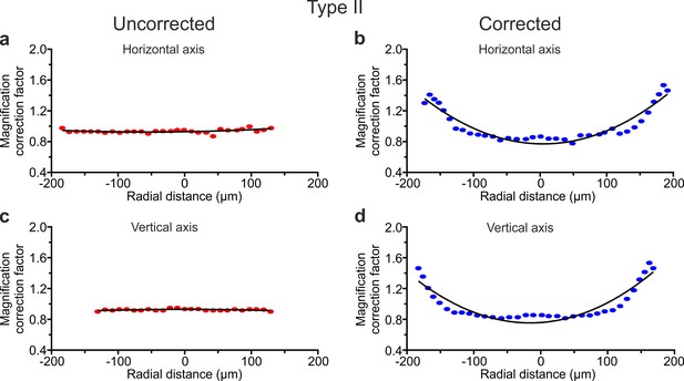
Field curvature in eFOV-microendoscopes.
(a,b) Magnification correction factor in the horizontal direction as a function of the radial position in uncorrected (a) and corrected (b) type II eFOV-microendoscopes. Plots show values obtained from one representative measurement. Dots represent experimental data. Black lines indicate quadratic polynomial fit. (c,d) Same as in (a,b) for the vertical direction.
-
Figure 3—figure supplement 4—source data 1
Magnification correction factor as a function of the radial position in uncorrected and corrected type II microendoscopes.
- https://cdn.elifesciences.org/articles/58882/elife-58882-fig3-figsupp4-data1-v3.xlsx
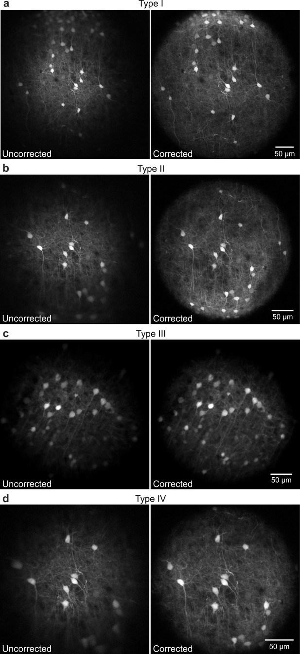
Corrected microendoscopes have extended effective FOV.
(a-d) Representative images of fixed cortical tissue expressing eGFP in neuronal cells acquired with type I (a), type II (b), type III (c), and type IV (d) microendoscopes without (uncorrected, left panels) and with (corrected, right panels) corrective lenses.
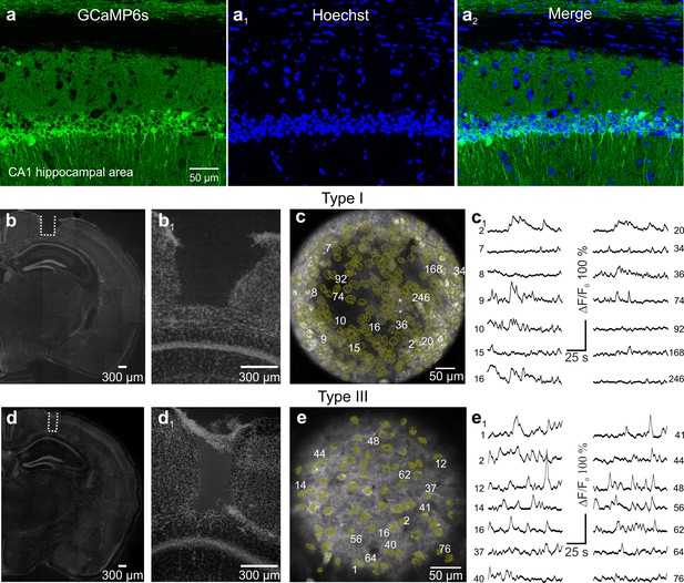
Hippocampal imaging with type I and type III eFOV-microendoscopes.
(a-a2), Confocal images of hippocampal CA1 neurons expressing GCaMP6s (a). Nuclei were counterstained with Hoechst (a1). Images are merged in (a2). Scale bar in (a) applies to a1-a2. (b-b1) Confocal images showing coronal slices from a mouse implanted with type I eFOV-microendoscopes. Slices were counterstained with Hoechst. The probe track is highlighted with the white dotted line in (b) and shown at a higher magnification in b1. (c-c1) GCaMP6s expressing CA1 hippocampal neurons recorded by two-photon imaging using type I eFOV-microendoscopes in an anesthetized mouse. ROIs are indicated by yellow lines. Examples of fluorescence change over time are shown in c1. (d-d1) Same as in (b–b1) but for type III eFOV-microendoscopes. (e–e1) Same as in (c–c1) but for type III eFOV-microendoscope.
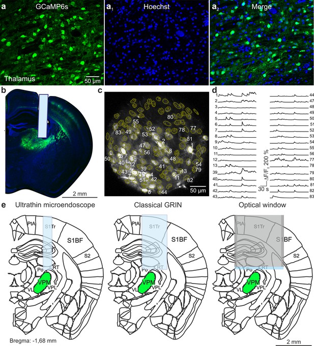
VPM imaging with type II eFOV-microendoscopes.
(a-a2) Confocal images of thalamic neurons expressing GCaMP6s (a). Nuclei were counterstained with Hoechst (a1). Images are merged in (a2). Scale bar in (a) applies to a1-a2. (b) Confocal image showing a coronal slice from a mouse implanted with a type II eFOV-microendoscope. The slice was counterstained with Hoechst. (c) GCaMP6s-expressing VPM neurons recorded using type II eFOV-microendoscopes in an awake head-restrained mouse. ROIs are indicated in yellow. (d) Fluorescence signals over time for some of the ROIs displayed in c. (e) Schematic showing the implantation of an ultrathin microendoscope (left), of a larger cross-section GRIN lens (middle), and of an optical window (right) for VPM imaging. S1BF = primary somatosensory, barrel field; S1Tr = primary somatosensory, trunk region; PtA = parietal association region; S2 = second somatosensory cortex; VPM = ventral posteromedial thalamic nucleus; RT = reticular thalamic nucleus; Po = posteromedian thalamic nucleus; VPL = ventral posterolateral thalamic nucleus; VL = ventrolateral thalamic nucleus.
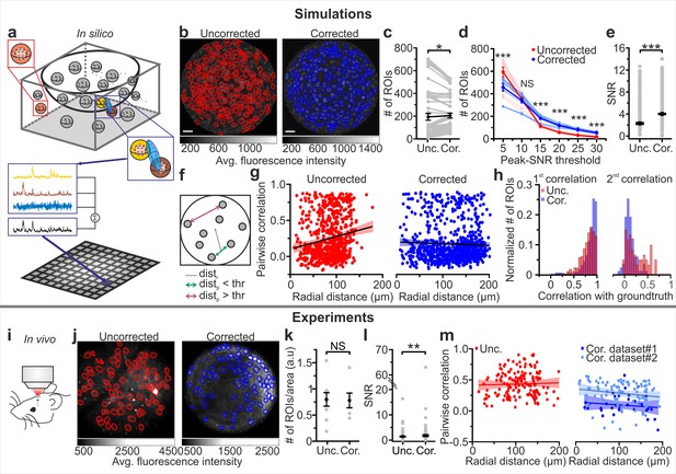
eFOV-microendoscopes allow higher SNR and more accurate evaluation of pairwise correlation.
(a) Schematic of the procedure for in silico simulation of imaging data. Neuronal activity was simulated within spheres located in a 3D volume, integrated over an elliptical PSF (blue) that was scanned on a curved FOV, projected on a 2D plane to generate artificial frames, and modulated through an intensity mask. Only voxels falling within the PSF contributed to the pixel signal (black trace). (b) Segmentation of in silico data for uncorrected (left, red lines indicate identified ROIs) and corrected (right, blue lines indicate identified ROIs) endoscopes. (c) Number of ROIs segmented in simulated FOVs for uncorrected (Unc.) and corrected (Cor.) microendoscopes. n = 54 segmentations from nine simulated FOVs, Wilcoxon signed-rank test, p=0.037. In this as well as in other figures, values from individual experiments are shown in gray, the average of all experiments in black and error bars indicate sem, unless otherwise stated. In this as well as in other figures: *p<0.05; **p<0.01; ***p<0.001; NS, not significant. (d) Number of segmented ROIs as a function of the peak-SNR threshold in artificial data from n = 9 simulated experiments. A two-way ANOVA with interactions showed a significant effect of peak-SNR threshold (p=1E-50) and of the interaction between peak-SNR threshold and probe type (p=1E-5) on the number of segmented ROIs, while the effect of probe type was not significant (p=0.096). (e) Average SNR of calcium signals under the different experimental conditions (peak-SNR threshold = 20 for the segmentation). n = 987 and 1603 ROIs for nine simulated experiments with uncorrected and corrected microendoscopes, respectively. Mann-Whitney test, p=5E-52. (f) Schematic representation of how radial distance (distr) and pairwise distance (distp) were calculated. (g), Pairwise correlation as a function of radial distance for simulated experiments with uncorrected (left) and corrected (right) microendoscopes. In this as well as other figures, lines show the linear regression of data. Shaded areas represent 95% confidence intervals. n = 738 and n = 869 pairwise correlations for uncorrected and corrected microendoscopes, respectively, from the n = 9 simulated experiments shown in (e). Linear regression fit of data: slope = 0.002, permutation test, p=0 and slope = −2E-4, permutation test, p=0.27 for uncorrected and corrected microendoscopes, respectively. (h) Distribution of the correlation of calcium signals with the first (left) or second (right) component of the ground truth for experiments with uncorrected and corrected microendoscopes. First component: n = 987 and 1603 ROIs for uncorrected and corrected microendoscopes, respectively, from n = 9 simulated experiments. Second component: n = 62 and 85 ROIs for uncorrected and corrected microendoscopes, respectively, from n = 9 experiments. (i) Schematic of the experimental configuration in awake animals. (j) Two-photon images of VPM neurons expressing GCaMP7f showing manually identified ROIs for uncorrected (left, red lines) and corrected (right, blue lines) type II microendoscopes. (k) Spatial density of ROIs identified in in vivo experiments. n = 9 FOVs and 6 FOVs from three animals with uncorrected and corrected microendoscopes, respectively. Student’s t-test, p=0.92. (l) SNR of segmented ROIs in in vivo recordings. n = 557 ROIs from 9 FOVs for uncorrected microendoscopes; n = 306 from 6 FOVs for corrected microendoscopes. Mann-Whitney test, p=0.0011. (m) Pairwise correlation as a function of radial distance for in vivo experiments. Number of pairwise correlations: n = 168 from 9 FOVs, n = 36 from 6 FOVs, and n = 92 from 24 FOVs for uncorrected, corrected (dataset 1), and corrected (dataset 2), respectively. Dataset two was obtained from experimental sessions performed during behavioral state monitoring as in Figure 6. Linear regression fit of data: slope = 0.0002, permutation test p=0.006 for uncorrected; slope = −0.0005, permutation test p=0.05 for dataset 1; slope = −0.0007, permutation test p=0.05 for dataset 2. See also Figure 4—figure supplements 1–2.
-
Figure 4—source data 1
Results of manual segmentation: # of ROIs, SNR, and pairwise correlations for simulated and experimental data.
Comparison between data obtained with uncorrected and corrected microendoscopes in silico and in vivo.
- https://cdn.elifesciences.org/articles/58882/elife-58882-fig4-data1-v3.xlsx

Manual vs. automated segmentation in simulated and experimental t-series.
(a), Recall values for the segmentation of simulated data in t-series obtained in uncorrected (red) and corrected (blue) microendoscopes for the manual (continuous line) and automated CaImAn (Giovannucci et al., 2019, dashed line) segmentation approaches (n = 9 simulations). (b) Same as in (a) for precision. (c) Same as in (a) for the F1 score. (d) Spatial density of ROIs identified in in vivo experiments using manual and automated segmentations for uncorrected microendoscopes. n = 9 FOVs from three animals. Paired Wilcoxon signed-rank test, p=4E-3. (e) Same as in (d) for corrected microendoscopes. n = 6 FOVs from three animals. Paired Wilcoxon signed-rank test, p=0.11.
-
Figure 4—figure supplement 1—source data 1
Comparison of manual vs automated segmentation methods in simulated and experimental data.
- https://cdn.elifesciences.org/articles/58882/elife-58882-fig4-figsupp1-data1-v3.xlsx

Improved description of neuronal signals in eFOV-microendoscopes is observed in t-series automatically segmented with CaImAn.
(a) Number of segmented ROIs as a function of the SNR threshold in artificial data from n = 9 simulated experiments. A two-way ANOVA with interactions showed a significant effect of SNR threshold (p=2E-24). Probe type and interaction effect were not significant (p=0.56 and 0.057 for probe type and for interaction, respectively). (b) Average SNR of calcium signals under the different experimental conditions (SNR threshold = 1 for the automatic CaImAn segmentation). n = 862 and 1378 ROIs in nine simulated experiments with uncorrected and corrected microendoscopes, respectively. Student’s t-test, p=0.01. (c) Pairwise correlation as a function of radial distance for simulated experiments with uncorrected (left) and corrected (right) microendoscopes. Solid lines indicate the linear regression of data and shaded areas represent 95% confidence intervals. n = 413 and n = 464 pairwise correlations for uncorrected and corrected microendoscopes, respectively, from the n = 9 simulated experiments shown in (b). Linear regression fit of data: slope = 1.8E-4, permutation test, p=7E-4 and slope = −1.5E-4, permutation test, p=0.38 for uncorrected and corrected microendoscopes, respectively. (d) SNR of segmented ROIs in in vivo recordings. n = 203 ROIs from 9 FOVs for uncorrected microendoscopes; n = 192 from 6 FOVs for corrected microendoscopes. Student’s t-test, p=0.38. (e) Pairwise correlation as a function of radial distance for in vivo experiments. Number of pairwise correlations: n = 30 from 9 FOVs, n = 26 from 6 FOVs for uncorrected and corrected microendoscopes, respectively. Linear regression fit of data: slope = 0.002, permutation test p=0.042 for uncorrected microendoscopes; slope = −4.7E-4, permutation test p=0.17 for corrected microendoscopes.
-
Figure 4—figure supplement 2—source data 1
Results of automated segmentation: # of ROIs, SNR, and pairwise correlations for simulated and experimental data.
- https://cdn.elifesciences.org/articles/58882/elife-58882-fig4-figsupp2-data1-v3.xlsx
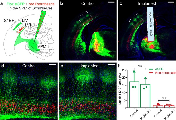
Ultrathin microendoscope implantation preserves thalamo-cortical and cortico-thalamic connectivity between S1bf and VPM.
(a) Local injection of red retrobeads and AAVs transducing floxed eGFP was performed in the VPM of Scnn1a-Cre mice. (b) Confocal image showing a coronal slice from an injected control animal. Scale bar: 500 μm. (c) Same as (b) but for a mouse implanted with a type II eFOV-microendoscope (probe diameter: 500 μm). (d,e) Zoom in of the S1bf region highlighted in (b,c). Scale bar: 100 μm. (f) Percentage of labeled S1bf area with eGFP (green) and retrobeads (red) in control and implanted mice. Points indicate the value of fluorescence from three mice (counted three coronal slices from each animal), column bars indicate average ± sd. One-tailed Mann-Whitney, p=0.20 for eGFP and p=0.50 for red retrobeads, respectively.
-
Figure 5—source data 1
Percentage of labeled S1bf area with eGFP and retrobeads in control and implanted mice.
- https://cdn.elifesciences.org/articles/58882/elife-58882-fig5-data1-v3.xlsx
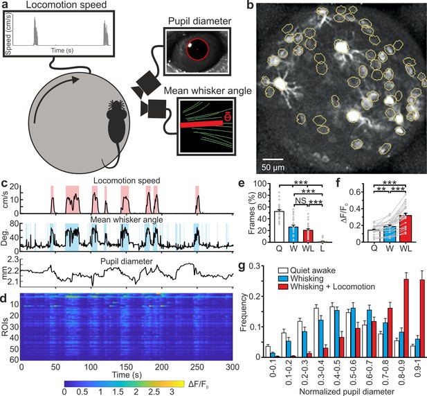
High-resolution population dynamics in the VPM of awake mice during locomotion and free whisking.
(a) Schematic of the experimental set-up for the recording of locomotion, whisker mean angle, and pupil size in awake head-fixed mice during VPM imaging using type II eFOV-microendoscopes. (b) Two-photon image of GCaMP6s labeled VPM neurons in vivo. (c) Representative traces of locomotion (top), whisker mean angle (middle), and pupil diameter (bottom). Red and blue shades indicate periods of locomotion and whishing, respectively (see Materials and methods for definition). (d), ΔF/F0 over time for all different ROIs in the experiment shown in (c). (e) Percentage of frames spent by the animal in quite wakefulness (Q), whisking (W), locomotion (L), and whisking + locomotion (WL). n = 24 time series from four animals. One-way ANOVA with Bonferroni post-hoc correction, p=3E-23. (f) Average ΔF/F0 across ROIs under the different experimental conditions. n = 24 time series from four animals. One-way ANOVA with Bonferroni post-hoc correction, p=2E-16. (g) Distribution of the Q, W, and WL states as a function of pupil diameter. Kolmogorov-Smirnov test for comparison of distributions of Q, W and WL states: p=0.07 for Q vs. W states, p=2E-10 for Q vs. WL states, p=1E-5 for W vs. WL states. For the statistical comparison of Q, W and WL states in each range of pupil diameter a two-way ANOVA with Tukey-Kramer post-hoc correction was performed; see Supplementary file 1 - Table 4. The error bars represent s.e.m across different t-series.
-
Figure 6—source data 1
Percentage of frames, ΔF/F0, and distribution of pupil diameter across behavioral states.
- https://cdn.elifesciences.org/articles/58882/elife-58882-fig6-data1-v3.xlsx
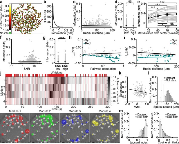
Cell-specific encoding of behaviorally-dependent information in distributed VPM subnetworks.
(a) Spatial map of neurons encoding whisking information. The pseudocolor scale shows significantly informative neurons (see Materials and methods). Data are pooled from 24 t-series from four animals. See also Figure 7—figure supplement 1. (b) Distribution of information content in individual ROIs. The individual ROIs information content distribution was fitted using a double exponential function (R2 = 0.99). n = 808 ROIs from 24 time series. (c) Information content of individual neurons vs. their radial distance from the center of the FOV. n = 842 neurons from 24 time series. Linear regression fit: slope = −3E-5, Student’s t-test p=0.13. Pearson correlation coefficient: −0.053, Student’s t-test p=0.13. (d) Information content for ROIs located at low radial distance (distr low) and in lateral portions of the FOV (distr high). n = 425 and 417 ROIs from 24 t-series for distr low and distr high, respectively. Mann-Whitney test, p=0.42. (e) Information content of neural populations as a function of the distance from the FOV center (% radius) used to include ROIs in the population. One-way ANOVA repeated measurements with Bonferroni post hoc, p=1E-18. Data pooled from 24 time series. (f) Information content of individual neurons vs. SNR. n = 842 neurons from 24 time series. Linear regression fit: slope = 9E-4, Student’s t-test p=2.7E-4. Pearson correlation coefficient: 0.125, p=2.7E-4. (g) Information content for ROIs with low SNR (SNR low) and high SNR (SNR high). n = 421 and 421 ROIs from 24 t-series for distr low and distr high, respectively. Mann-Whitney test, p=5E-5. (h,i) Synergistic (gray) or redundant (dark green) information within pairs of neurons is shown as a function of pairwise correlation (h) and as a function of radial distance (i). n = 61 and 31 pairs of neurons for synergistic and redundant information content, respectively. Data from 24 time series. Linear regression fit in (h): slope = 0.008, permutation test p=0.45 and slope = −0.02, permutation test p=0 for synergistic and redundant information, respectively. Linear regression fit in (i): slope = −0.0001, permutation test p=0.007 and slope = 2E-5, permutation test p=0.38 for synergistic and redundant information, respectively. (j) Top: representative grayscale matrix showing the activation coefficient across time for 4 NMF modules emerging in a FOV containing 37 neurons. Periods of whisking are shown in red bars and shades. Bottom: ROIs belonging to the four different modules shown in the top panel. Each colored circle represents a ROI belonging to the specified module and its radius is proportional to the ROI weight within that module. The corresponding activation coefficients are presented in the upper panel. (k) Module sparseness as a function of the whisking modulation index (WMI). n = 213 modules from 24 time series. Pearson correlation coefficient: −0.164, p=0.016. (l) Normalized number of modules as a function of their spatial spread for the experimental data (gray) and for a null distribution obtained by randomly shuffling the spatial position of ROIs in the FOV (white). Number of modules: n = 213 and n = 2400 for the 24 t-series of the in vivo dataset and for the null distribution, respectively. (m) Left: Normalized number of modules as a function of their Jaccard index for pairs of modules identified within the same FOV for experimental data (gray) and for a null distribution (white) obtained by randomly shuffling the spatial position of ROIs within the FOV. Number of modules: n = 1704 and n = 34080 for the 24 t-series of the experimental data and for the null distribution, respectively. Right: same as in the left panel for Cosine similarity coefficients.
-
Figure 7—source data 1
Information theoretical analysis and non-negative matrix factorization results.
Values of cell-specific and population information analysis.
- https://cdn.elifesciences.org/articles/58882/elife-58882-fig7-data1-v3.xlsx
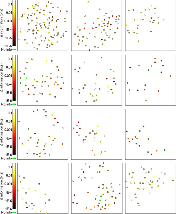
Cell-specific encoding of behavioral state-dependent information in distributed VPM subnetworks.
Spatial map of neurons encoding whisking information in 12 out of the total 24 analyzed time series. The pseudocolor scale shows significantly informative neurons (see Materials and methods).
Tables
| Reagent type (species) or resource | Designation | Source or reference | Identifiers | Additional information |
|---|---|---|---|---|
| Strain, strain background (M. musculus) | C57BL/6J | Charles River | RRID:IMSR_JAX:000664 | |
| Genetic reagent (M. musculus) | B6;C3-Tg(Scnn1a- cre)3Aibs/J | The Jackson Laboratory | RRID:IMSR_JAX:009613 | |
| Recombinant DNA reagent | pAAV.Syn.Flex. GCaMP6s.WPRE.SV40 | Penn Vector Core | RRID:Addgene_100845; Addgene viral prep # 100845-AAV1 | Chen et al., 2013 |
| Recombinant DNA reagent | pGP-AAV-syn- FLEX-jGCaMP7f-WPRE | Addgene | RRID:Addgene_104492; Addgene viral prep # 104492-AAV1 | Dana et al., 2016 |
| Recombinant DNA reagent | AAV pCAG- FLEX-EGFP-WPRE | Penn Vector Core | RRID:Addgene_51502; Addgene viral prep # 51502-AAV1 | Oh et al., 2014 |
| Recombinant DNA reagent | AAV.CaMKII0.4. Cre.SV40 | Penn Vector Core | RRID:Addgene_105558; Addgene viral prep # 105558-AAV1 | |
| Commercial assay or kit | Kwik-Cast | World Precision Instruments | Cat# KWIK-CAST | |
| Commercial assay or kit | Sylgard Silicone Elastomer | Dow Inc | Cat# Sylgard 164 | |
| Commercial assay or kit | Norland Optical Adhesive 63 | Norland | Cat# NOA 63 | |
| Commercial assay or kit | GRIN lens | Grintech | Cat# NEM-050- 25-10-860-S | |
| Commercial assay or kit | GRIN lens | Grintech | Cat# NEM-050- 43-00-810-S-1.0p | |
| Commercial assay or kit | GRIN lens | Grintech | Cat# GT-IFRL-035- cus-50-NC | |
| Commercial assay or kit | GRIN lens | Grintech | Cat# NEM-035- 16air-10–810 S-1.0p | |
| Chemical compound, drug | bisBenzimide H 33342 trihydrochloride (Hoechst) | Sigma-Aldrich | Cat# B2261; CAS: 23491-52-3 | |
| Chemical compound, drug | Red Retrobeads | LumaFluor Inc | Red Retrobeads | |
| Software, algorithm | Zemax OpticStudio 15 | Zemax | https://www.zemax.com/products/opticstudio | |
| Software, algorithm | MATLAB R2017a | Mathworks | RRID:SCR_001622; https://it.mathworks.com/products/matlab.html | |
| Software, algorithm | GraphPad PRISM | GraphPad PRISM | RRID:SCR_002798; https://www.graphpad.com/ | |
| Software, algorithm | ImageJ/Fiji | Fiji | RRID:SCR_002285; http://fiji.sc/ | |
| Software, algorithm | NoRMCorre | Pnevmatikakis and Giovannucci, 2017 | https://github.com/flatironinstitute/NoRMCorre | |
| Software, algorithm | CaImAn | Giovannucci et al., 2019 | https://github.com/flatironinstitute/CaImAn-MATLAB | |
| Software, algorithm | Population Spike Train Factorization Toolbox for Matlab Version 1.0 | Onken et al., 2016 | https://stommac.eu/index.php/code | |
| Software, algorithm | LIBSVM | Chang and Lin, 2011 | https://www.csie.ntu.edu.tw/~cjlin/libsvm/ | |
| Software, algorithm | Information Breakdown ToolBox | Magri et al., 2009 | N/A | |
| Software, algorithm | Software used in this paper for generation of artificial time series | https://github.com/moni90/eFOV_microendoscopes_sim | Figure 4a–h, Figure 4—figure supplement 1a–c and Figure 4—figure supplement 2a–c | |
| Software, algorithm | Software to compute recall, precision, and F1 score | Soltanian-Zadeh et al., 2019 | https://github.com/soltanianzadeh/STNeuroNet | |
| Other | Basler ace camera | Basler AG | Cat# acA800-510um | |
| Other | Optical encoder | Broadcom | AEDB-9140-A13 | |
| Other | Zortrax M200 3D printer | Zortrax | M200 | |
| Other | Z-ULTRAT 3D printer filament | Zortrax | Z-ULTRAT | |
| Other | Arduino Uno | Arduino | Arduino Uno |
Additional files
-
Supplementary file 1
Characteristics of eFOV-microendoscopes and their application in awake mice.
Supplementary Table 1: Parameters for the fabrication of corrective lenses. Coefficients used in Equation (1) (see Materials and methods) for the aspherical corrective lenses used in type I-IV eFOV-microendoscopes. Supplementary Table 2: Simulated focal length in uncorrected and corrected microendoscopes. Supplementary Table 3: Spatial resolution and effective FOV of eFOV-microendoscopic probes. Values are reported as average ± sem. For statistical comparison of uncorrected (uncor.) vs. corrected (cor.) microendoscopes, Student’s t-test was used. Supplementary Table 4: Statistical comparisons of behavior state distributions as a function of pupil diameter. For the statistical comparison of Q, W, and WL state distributions in each range of pupil diameter, a two-way ANOVA with Tukey-Kramer post-hoc correction was performed.
- https://cdn.elifesciences.org/articles/58882/elife-58882-supp1-v3.docx
-
Transparent reporting form
- https://cdn.elifesciences.org/articles/58882/elife-58882-transrepform-v3.docx


