How many neurons are sufficient for perception of cortical activity?
- Wolfson Institute for Biomedical Research, University College London, United Kingdom
Figures
Figure 1 with 6 supplements
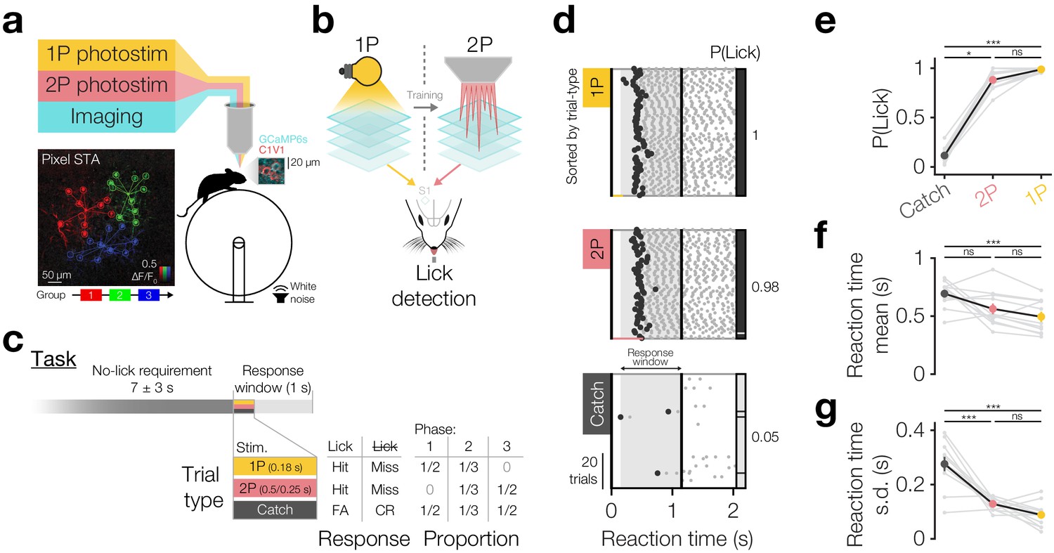
Driving behaviour with two-photon optogenetics targeted to ensembles of neurons in L2/3 barrel cortex.
(a) Schematic of all-optical setup. Bottom left: Example of flexible ensemble photostimulation. Three 10 neuron groups in barrel cortex (red, green, blue circles joined by group centroids) were photostimulated sequentially (sequence below Pixel STA). Pixel STA is maximum intensity projection across photostimulus groups of activity in post-photostimulation epoch averaged across trials (N = 3 photostimulus groups, 10 trials each). Inset right: sub-region of a full imaging FOV in L2/3 barrel cortex expressing GCaMP6s/C1V1-mRuby. (b) Schematic summarising the strategy used to train animals to respond to two-photon optogenetic (2P) stimulation. Mice are first trained to respond to one-photon optogenetic (1P) stimulation of barrel cortex (S1) by licking at an electronic lickometer. The power of 1P illumination is reduced until they can be transitioned onto 2P stimulation targeted to specific ensembles of barrel cortex neurons. (c) Structure of the behavioural task (top) and stimulus probabilities, response type contingencies and training phase structures (bottom). Note that stimulus durations, which vary across stimulus types, are not to scale. FA: false alarm; CR: correct reject. (d) Lick raster from an example Phase 2 behavioural training session during which a mouse received 2P stimulation trials (pink: 200 neurons), catch trials (grey: no stimulus) and 1P stimulation trials (amber: 0.05 mW, untargeted). Trials were delivered pseudo-randomly (see Materials and methods) but have been sorted by trial type for display. All licks shown in grey with first lick highlighted in black. Hits/false alarms (black) and misses/correct rejects (grey) are indicated as the vertical bar on the right-hand side. Stimulus durations indicated as coloured bars below lick rasters. Behavioural response window indicated as grey shading, label and arrows. (e–g), Response rate and reaction time mean and standard deviation for different trial types in final Phase 2 session. Animals detect 1P photostimulation and 2P stimulation targeted to 200 neurons to similar extents, at a level far above chance (catch trials), with similar reaction time mean and standard deviation. (N = 12 mice, 1 session each). Note only animals which responded on >2 catch trials are included for reaction time panels (f and g) (N = 11 mice, 1 session each). All error bars are s.e.m.
Figure 1—figure supplement 1
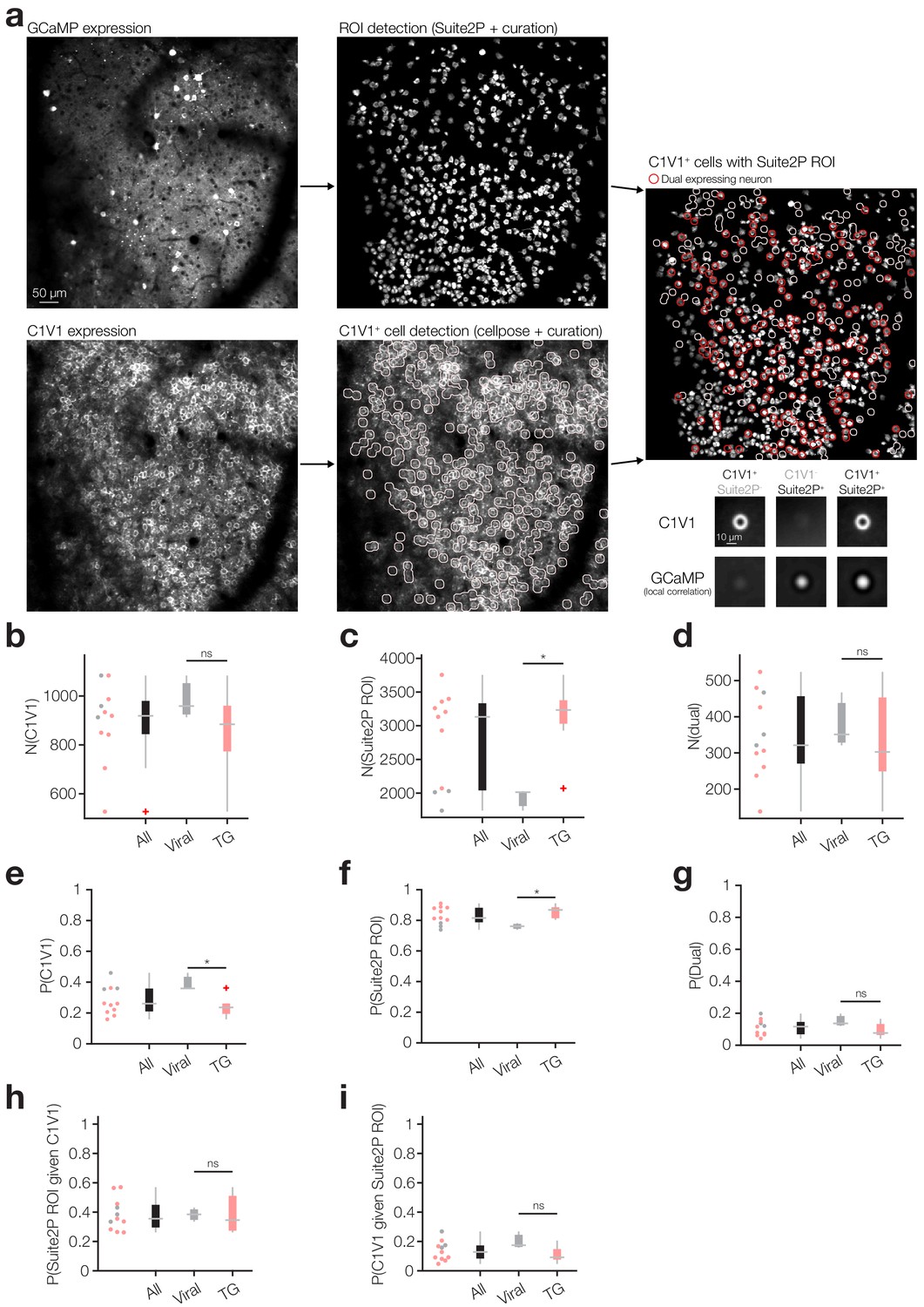
Indicator and opsin expression overlap analysis.
(a) Detection of indicator/opsin expression overlap. Suite2P followed by manual curation was used to detect functional GCaMP-expressing neurons from time-series data (top row) and Cellpose followed by manual curation was used to detect C1V1 expression from static images (bottom row). GCaMP (top left) and C1V1 (bottom left) expression in an example plane from a volumetric FOV with corresponding Suite2P ROIs (top middle) and detected C1V1+ neurons (bottom middle). C1V1+ neurons with a Suite2P ROI are circled in red (right; see Materials and methods) and the average expression pattern in both C1V1 expression and GCaMP local correlation images is shown for each of the three possible expression configurations (bottom right insets). N = 6250 C1V1+/Suite2P- neurons, 27084 C1V1-/Suite2P+ neurons and 3810 C1V1+/Suite2P+ neurons across 11 volumetric FOVs from 6 mice, 1–2 volumetric FOVs each. (b) Number of C1V1+ neurons in each volumetric FOV in all mice (black), dual injected WT mice (grey) and opsin injected transgenic GCaMP mice (pink). See below and Materials and methods for details. (c) Number of Suite2P ROIs in each volumetric FOV. (d) Number of dual expressing neurons in each volumetric FOV (C1V1+ neurons with Suite2P ROI). (e) Proportion of C1V1+ neurons out of total number of neurons that have a Suite2P ROI and/or are C1V1+. (f) Proportion of neurons with a Suite2P ROI out of total number of neurons. (g) Proportion of dual expressing neurons (C1V1+ with Suite2P ROI) out of total number of neurons. (h) Proportion of C1V1+ neurons with a Suite2P ROI. (i) Proportion of Suite2P ROIs that are C1V1+. For all group data panels N = 11 volumetric FOVs from the 2P psychometric curve sessions (Figures 2, 3 and 4), 3 FOVs from WT (C57/BL6) mice co-injected with hSyn-GCaMP6s/CaMKII-C1V1-Kv2.1 (grey in all plots) and 8 FOVs from transgenic (Emx1Cre;CaMKIIa-tTA;Ai94) mice injected with CaMKII-C1V1-Kv2.1 (pink in all plots). Aggregate data across expression strategies are black in all plots. All boxplots indicate median (horizontal line) and 25th and 95th percentiles (box) with whiskers extending to the most extreme data not considered outliers (see Materials and methods) and outliers indicated in red beyond.
Figure 1—figure supplement 2
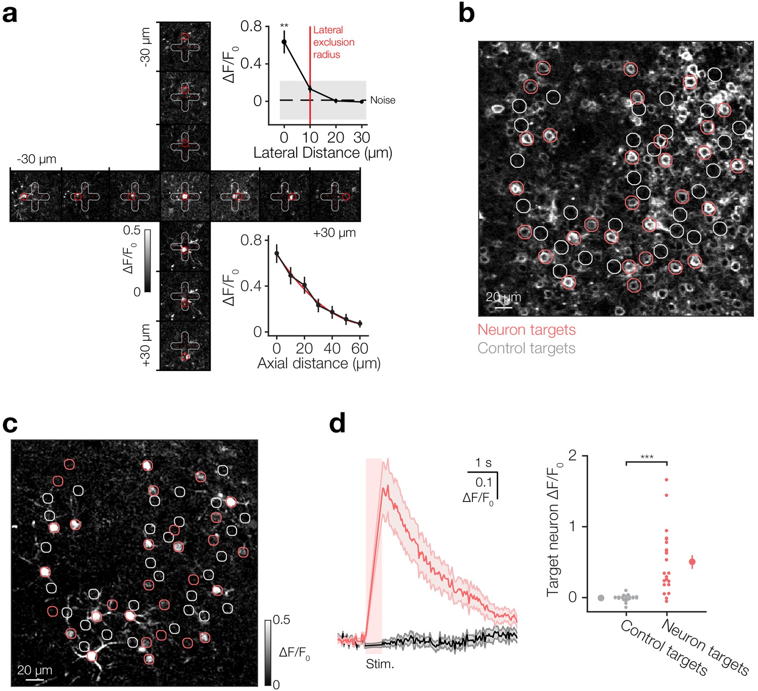
Spatial resolution of spiral-scanned two-photon optogenetic activation of Kv2.1-C1V1.
(a) Left: A cross-shaped grid of photostimulation targets was centred on a single target neuron and each photostimulation target was activated 10 times in random order (10 µm inter-target distance, 30 µm maximum distance from centre, 10 s inter-trial interval, 10 × 20 ms spirals at 20 Hz, 6 mW/neuron). Top right inset: Lateral (xy) resolution of photostimulation of the central target neuron. Only the target position centred over the target neuron result in significant activation. Lateral HWHM = 5 µm (two-degree polynomial fit). N = 1 neuron, 10 trials per stimulation site. Note the lateral exclusion radius (10 µm) used to define target neurons in subsequent analyses is plotted in red. All neurons within this region were considered potential target neurons (see Materials and methods). Bottom right inset: Axial (z) resolution of photostimulation. Photostimulation targets were axially translated from 60 µm above target neurons down onto their cell-body locations in the objective focal plane in 10 µm steps using SLM-based axial displacement while the target neuron responses were consistently imaged at the objective focal plane (separate experiments from lateral resolution). HWHM = 20 µm (two-degree polynomial fit). N = 20 neurons, 10 trials per axial offset. To account for these considerable axial off-target effects we defined all neurons within the lateral exclusion zone of 10 µm (see above) to be potential target neurons irrespective of their axial displacement. (b) Example Kv2.1-C1V1-mScarlet expression image with neuron (pink) and control (grey) targets overlaid as circles. (c) Maximum intensity projection across two pixel-wise STAs triggered off neuron and control site stimulation. Neuron stimulation results in robust activation of targeted neurons, control stimulation results in no activation. N = 10 trials. (d) Left: Extracted traces from target neuron ROIs during both neuron site stimulation (pink) and control site stimulation (grey). Right: post-stimulus ∆F/F0 from target neuron ROIs. Transients evoked in target neuron ROIs during neuron site stimulation are completely absent during stimulation of adjacent control sites, resulting in no recorded ∆F/F0 response. N = 20 neurons, 10 trials each. All error bars and shading are s.e.m. unless otherwise stated.
Figure 1—figure supplement 3
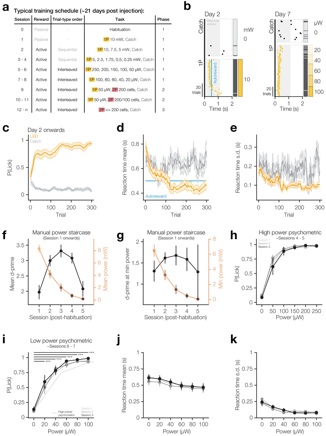
1P training protocol.
(a) Typical training protocol to transition a naïve mouse to being able to detect two-photon stimulation via a series of one-photon priming phases. Note that exact duration of each component varied by mouse (see Figure 1—figure supplement 5f). (b) Lick rasters from an example first training session (left) and an example low power psychometric curve session (right) for a habituated mouse showing first licks on each trial (circles), auto-reward delivery time (blue vertical line) and analysis window (grey shading). Trials were delivered pseudorandomly and are sorted for display only. Hits (black) and misses (grey) are indicated as the vertical bar to the right of the raster, followed by coloured boxes indicating LED power on the far right. (c–e) Moving average response rate (c), average reaction time (d) and standard deviation of reaction time (e) for the first 300 LED (amber) and catch (grey) trials using a 20 trial window. (f) Mean power (right) and mean d-prime (left) over initial manual power staircase sessions. (g) Minimum power used in each session (right) and d-prime at that power (left) over initial manual power staircase sessions. (h) Response rates on three high-power psychometric curve sessions. N = 22 mice that completed at least one high-power psychometric curve session (other animals were transitioned straight to low-power psychometric curves). (i–k), Response rates (i), mean reaction time (j) and standard deviation of reaction time (k) on three low-power psychometric curve sessions. N = 22 mice that completed at least one low-power psychometric curve session (other animals were transitioned straight to subsequent training phases). All error bars and shading are s.e.m. For all group data panels, N = 26 mice unless otherwise stated, however some data-points may have fewer N as not all animals completed the same number of sessions (see Figure 1—figure supplement 5f for summary).
Figure 1—figure supplement 4
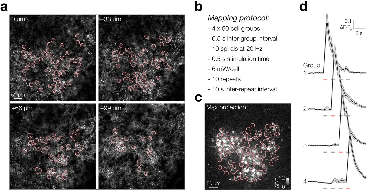
Example pre-training selection and mapping of 200 neurons in L2/3 barrel cortex.
(a) Kv21-C1V1-mScarlet expression from an example four-plane imaging volume with stimulation targets overlaid in pink. Neurons are chosen arbitrarily, with the only criteria being that neurons are expressing C1V1 and not too far from FOV centre. Depths relative to most superficial plane (~130 µm below pia). (b) Pre-training mapping protocol used to assess photostimulatability. Note 200 neurons are mapped in 4 × 50 neuron groups. (c) Example pixel-wise STA maximum intensity projected across the four stimulation groups and the four planes with targets overlaid in pink. (d) Trial-averaged STA traces from ROIs in (c), 50 neurons per group. Note the temporal offset (0.5 s) between activation of each group. Shading denotes s.e.m. N = 1 FOV, 1 animal, 200 neurons, 10 trials.
Figure 1—figure supplement 5
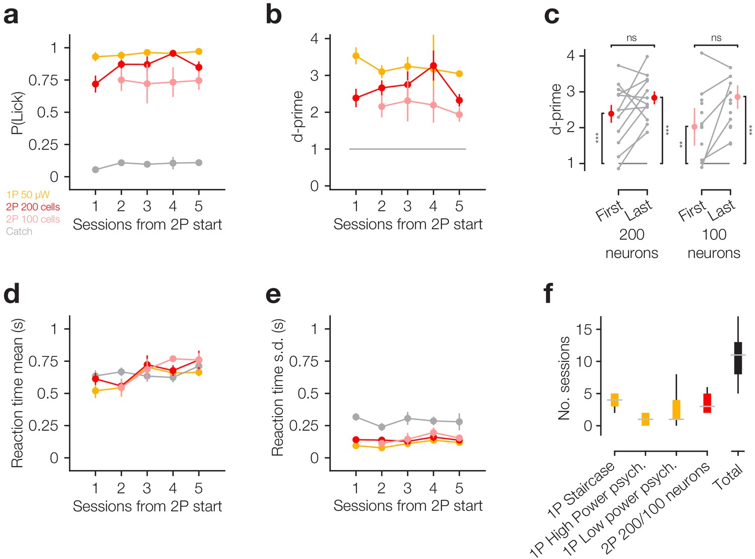
Rapid transfer learning from 1P to 2P optogenetic stimuli.
(a – b) Response rates for different 1P and 2P stimulus types from the first session using 2P stimuli, quantified as proportion of trials where animal licked (a) and d-prime relative to catch trials (b). Note that this includes a combination of Phase 2 (LED/2P/catch trials) and Phase 3 (2P/catch trials) sessions. (c) Quantification of d-prime relative to our learning criterion (d-prime >1) for the first and last session using 2P stimuli of different magnitudes. Note that some animals only had one session using 2P stimulation of 100 neurons. This session is duplicated in the First and Last tests against d-prime >1, but not included in the test for improvement over time. As such these data points appear as grey dots that are not joined by horizontal grey lines. (d–e) Reaction time mean (d) and standard deviation (e) for different trial types from the first session using 2P stimuli. Trial types with <3 responses were excluded from reaction time analyses. (f) Number of sessions of each step in the training paradigm (coloured bars) and total number of sessions from beginning of 1P training to end of initial 2P training (black bar). For all plots maximum N = 12 mice, although individual data-points may have less as not all animals had the same number of training sessions. All error bars are s.e.m.
Figure 1—figure supplement 6

Comparison of behavioural response to somatic and non-somatic C1V1.
(a) Animals detect stimulation of somatic and non-somatic C1V1 to similar extents. (b) Animals respond slightly quicker to stimulation of non-somatic C1V1. (c) Reaction times are similarly consistent across somatic and non-somatic C1V1. All error bars are s.e.m. N = 12 C1V1-Kv2.1 mice, 19 C1V1 mice.
Figure 2 with 3 supplements
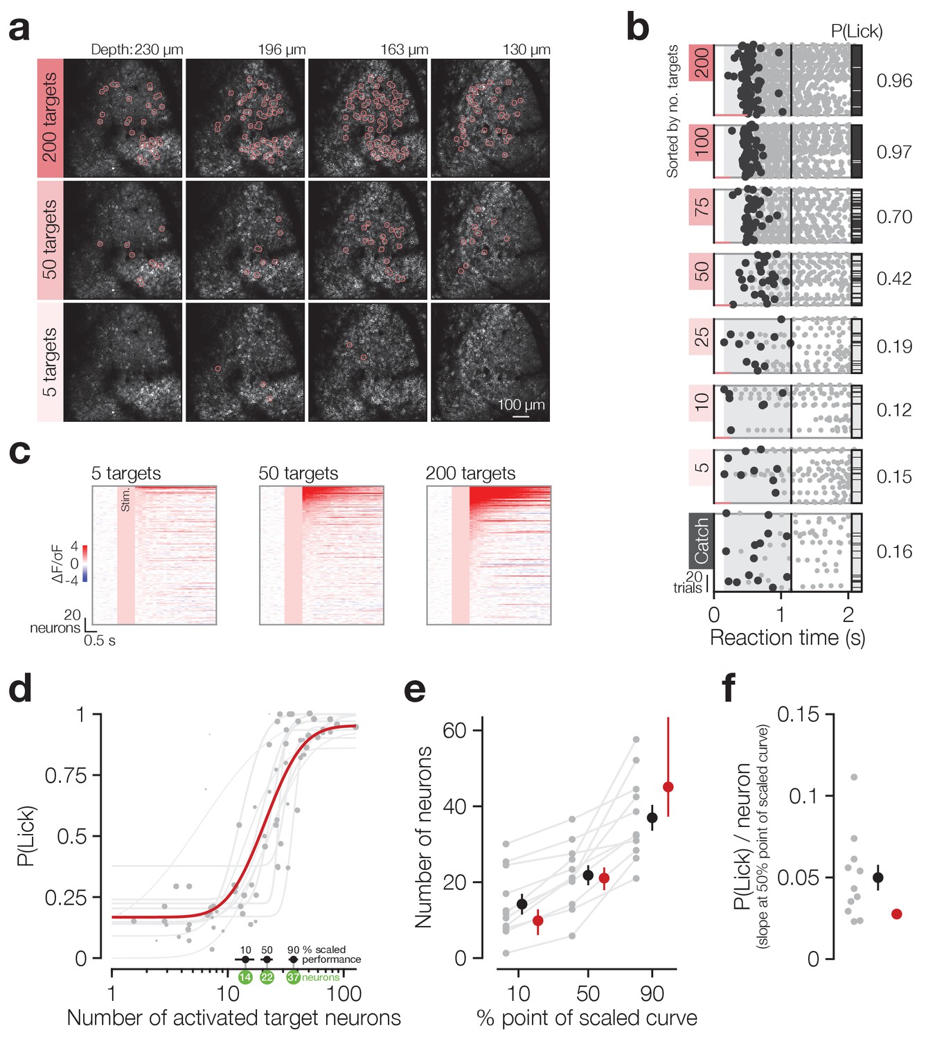
Animals detect the targeted activation of tens of neurons.
(a) Example imaging volumes from an experiment showing 200 (top), 50 (middle) and 5 (bottom) targeted C1V1-expressing neurons. (b) Example lick raster concatenating an animal’s two psychometric curve testing sessions. Trials were delivered pseudo-randomly (see Materials and methods) but have been sorted by trial type for display. Stimulus durations are indicated by coloured bars along the bottom of each raster. Animals respond on more trials and with less variable timing as more neurons are targeted. (c) Example responses across the top 200 most responsive neurons in the 200 target zones (see Materials and methods; Figure 2—figure supplement 1). Neurons have been sorted separately in each plot. Pink boxes indicate the stimulus artefact exclusion epoch which is consistent across all trial types (see Materials and methods for definition). (d) The psychometric function relating the number of activated target neurons to the behavioural detection rate for all 2P psychometric curve sessions. Individual data (grey dots) are grouped by trial type within session (number of target zones) and plotted as the average number of target neurons activated across all trials of each type. Data point size indicates the number of trials of each type (29 ± 8 trials, range 11–44, across data points). Individual psychometric curve fits for each session are plotted (grey lines) weighted by the total number of stimulus trials in the session (202 ± 50 trials, range 97–245, across sessions). The number of neurons required to reach the 10%, 50% and 90% points of these individual scaled psychometric curves are shown as black error bars and green circles about the x-axis. The aggregate psychometric curve fit across all trial types, all sessions, is plotted in red. Note that individual curves are often steeper than the aggregate curve. (e) The number of neurons required to reach the 10%, 50%, and 90% points of the scaled psychometric curves in (d). Grey data points/lines are quantified from individual psychometric curve fits (grey lines in d) and summarised by the black error bars. Red data points are quantified from the aggregate psychometric curve fit (red line in d) ± confidence intervals. (f) The slope at the 50% point of the scaled curves corresponding to the additional probability of detection (P(Lick)) added per target neuron activated. Grey data points are quantified from individual psychometric curve fits (grey lines in d) and are summarised by the black error bar. The red circle is quantified from the aggregate psychometric curve fit (red line in d) for which no confidence intervals can be calculated (see Materials and methods). N = 11 sessions, 6 mice, 1–2 sessions each. All data error bars are mean ± s.e.m. and all fit parameter error bars are estimate ± confidence intervals.
Figure 2—figure supplement 1
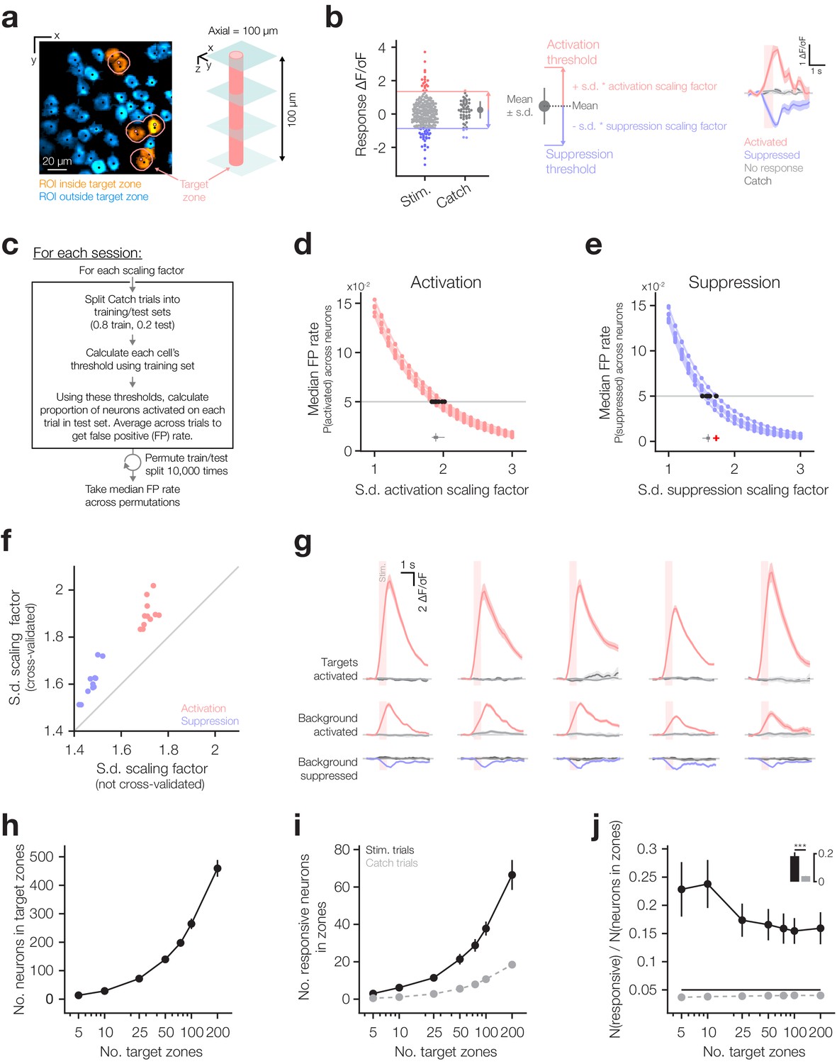
Quantification of neuronal responses.
(a) Example target zones. Left: section of a plane in a volumetric FOV showing Suite2P ROIs (coloured regions), Suite2P centroids (black dots), target co-ordinates (pink dots) and lateral extent of target zone (pink circles; 10 µm radius). ROIs with centroids within the target exclusion zones are considered potential targets (orange ROIs), ROIs outside these regions are considered background neurons (blue ROIs). Right: schematic illustrating axial extent of target zone. (b) Rationale behind activation and suppression thresholds calculated from correct reject (CR) catch trial responses and illustration of the results of our threshold procedure (described in c–e). Left: trial-wise responses for a single non-target neuron on stimulus trials of all types and CR catch trials. The mean and standard deviation of responses on CR catch trials can be used to infer activation and suppression thresholds that separate stimulus evoked activation (red) and suppression (blue) responses from the majority of CR catch trial responses. Middle: activation and suppression thresholds are computed as the mean + or – the standard deviation respectively, scaled by a scaling factor (separate scaling factors for activation and suppression). Right: average responses on trials where this neuron was activated (red), suppressed (blue) or unresponsive (light grey). Catch trials are also included (dark grey). Such a procedure separates positive and negative going responses from non-responsive trials which should themselves be indistinguishable from catch trials. (c) Procedure for inferring cross-validated positive and negative standard deviation scaling factors that yield a 5% false positive response rate on catch trials for each session’s volumetric FOV. For each session’s data, and each threshold type (i.e. activation threshold), we sweep through a series of scaling factors. For each factor we permute a 80:20 train:test split of correct reject (CR) catch trials 10,000 times. On each permutation, we use the scaling factor and that permutation’s training CR catch trials to calculate each neuron’s threshold. Using these neuron-wise thresholds, we then compute the proportion of neurons activated on each testing CR catch trial and average across trials (false positive rate; FP). We then take the median FP across all permutations at this scaling factor before moving to the next scaling factor. We can then infer the scaling factor that yields a 5% FP rate on testing CR catch trials across permutations. (d) Relationship between standard deviation scaling factor and FP rate for the activation threshold. Data points are empirically quantified values, fits are cubic interpolations. The optimal scaling factor for each experiment (horizontal boxplot) is inferred by finding the scaling factor for which the fitted FP rate is 5% (horizontal line). (e) Relationship between the standard deviation scaling factor and FP rate for the suppression threshold. Data conventions and scaling factor inference the same as (d). (f) Scaling factors that yield 5% false positive rate when all correct reject catch trials are used (not cross-validated, i.e. thresholds inferred and tested on same trials) compared to those yielded by the cross-validation procedure described in (c–e). Cross-validation yields more stringent thresholds. (g) Example traces from one session for five activated target neurons (top row), five activated background neurons (middle row) and five suppressed background neurons (bottom row) illustrating responses yielded by our procedure. Averages across all activated/suppressed trials are shown in red/blue and averages across catch trials/non-responsive stimulus trials are shown in light and dark grey, respectively. Note that neurons in each column are unrelated. (h) The number of neurons in all target zones for each trial type (as defined in (a) and Materials and methods). (i) The number of responsive neurons in all target zones for each trial type on both stimulus trials (black) and catch trials (grey). (j) Proportion of responsive neurons in all target zones for each trial type on both stimulus trials (black) and catch trials (grey) quantified as the number of responsive neurons in target zones (i) divided by the number of neurons in target zones (h). Inset: Proportion of target zone neurons that are responsive on stimulus trials compared to catch trials. N = 11 sessions, 6 mice, 1–2 sessions each for all group data plots. Error bars and shading are s.e.m.
Figure 2—figure supplement 2
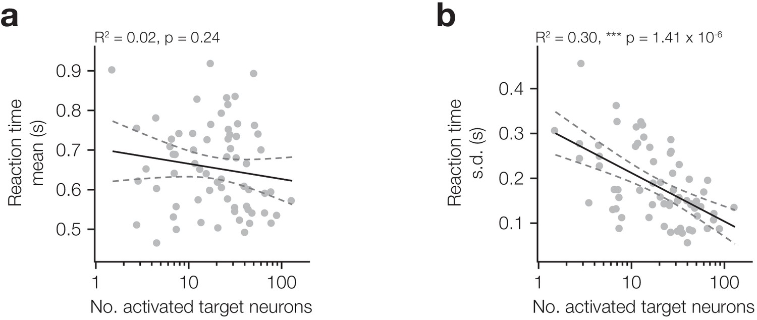
Reaction time standard deviation, but not mean, scales with the number of target neurons activated.
(a–b) Relationship between mean (a) and standard deviation (b) of reaction time and the number of activated target neurons.
Figure 2—figure supplement 3
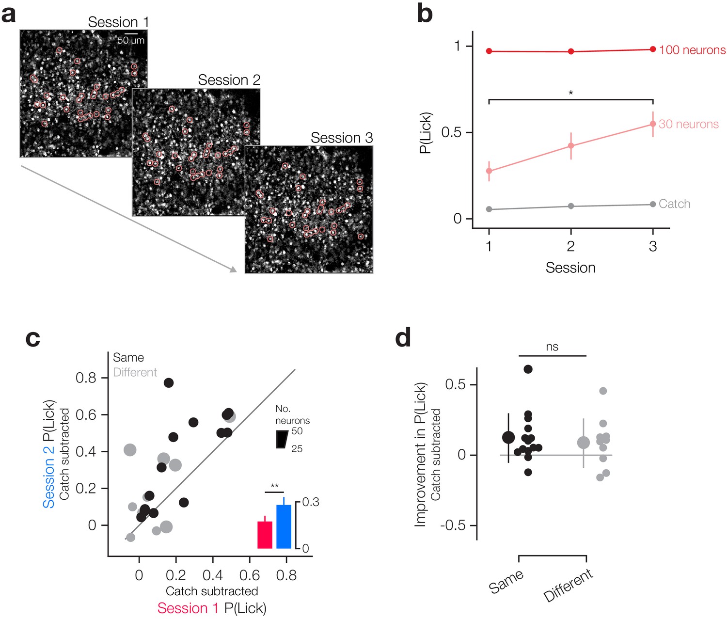
Detection of small ensembles of neurons improves across days irrespective of whether the same neurons were targeted.
(a) FOV from training sessions across 3 consecutive days where we stimulated the same 30 neurons each day. (b) Average behavioural response rates for 100 neuron, 30 neuron and catch trial conditions for all sessions where we stimulated the same neurons across days (N = 14 mice). (c) Improvement in response rates from session 1 to session 2. Sessions in which we targeted the same neurons are shown in black and sessions where we targeted different neurons in grey. Data-point size denotes number of targeted neurons, scale inset (same neurons group N = 14 mice, different neurons group N = 5 mice, 2 stim types each). (d) Sessions targeting the same neurons showed a similar amount of improvement as sessions targeting different neurons (same neurons group N = 14 mice, different neurons group N = 5 mice, two stim types each). All error bars are s.e.m.
Figure 3 with 3 supplements

Increasing target activation is matched by background network suppression.
(a) The proportion of neurons activated across all neurons (targets and background) increases as more target neurons are activated. Inset right: average activation across all trial types is increased on stimulus trials compared to catch. (b) The proportion of neurons suppressed across all neurons (targets and background) increases as more target neurons are activated. Inset right: average suppression across all trial types is increased on stimulus trials compared to catch. (c) The ratio of activation and suppression is similar to that observed on catch trials (inset right) and is not strongly modulated by the number of activated target neurons. (d) Stimulation of target neurons causes mild activation of background neurons (targets excluded; inset right) but this is not modulated by the number of target neurons activated. (e) Stimulation of target neurons causes suppression of background neurons (targets excluded; inset right) which increases as more target neurons are activated. All data are hit:miss matched to remove potential lick signals (see Figure 3—figure supplement 1 and Materials and methods). For all plots N = 11 sessions, 6 mice, 1–2 sessions each. Some trial types from some sessions are excluded for having too few hits or misses to be able to match the hit:miss ratio. Error bars and shading are s.e.m; data points, error bars and linear fits are stimulus trials, shading is catch trials; grey data points: individual trial types, individual sessions; coloured error bars: data averaged within trial type (number of target zones) across sessions; linear fits are to individual data points; fits are reported ± 95% confidence intervals.
Figure 3—figure supplement 1
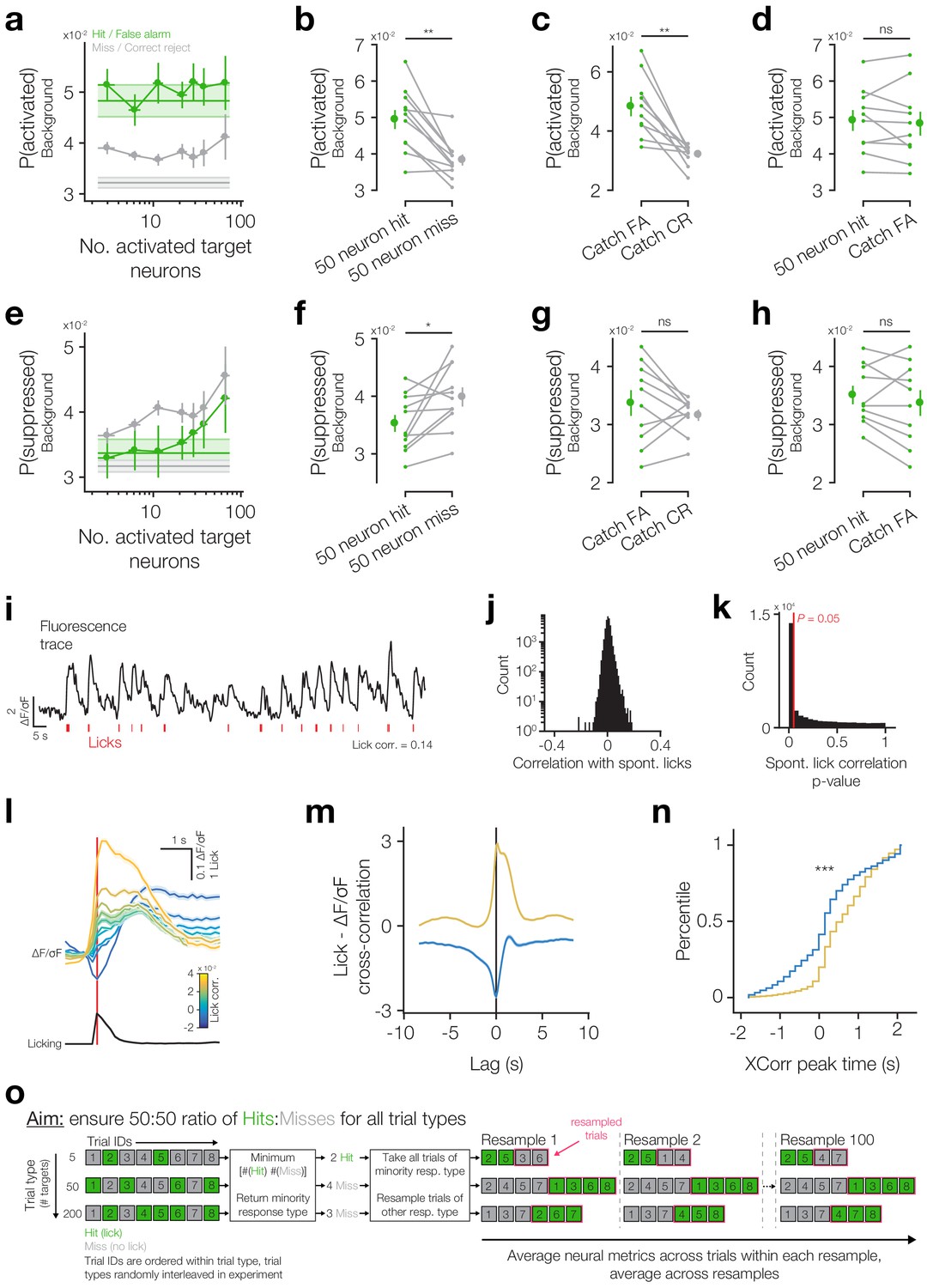
Comparison of network activity on hits and misses for both threshold go trials and catch trials in an effort to quantify and account for lick responses.
(a) The proportion of background neurons activated when different numbers of target neurons are activated on hits/false alarms (green) and misses/correct rejects (grey) on stimulus trials (error bars) and catch trials (shading). Background neurons become more active on stimulus hits and catch false alarms and there does not seem to be much modulation of the amount of background activation by the number of activated target neurons. Note that the background neuron activation response on stimulus trials overlaps with the response on catch trials across the full range of number of target neurons activated. (b) The proportion of activated background neurons is higher on stimulus hit trials than miss trials. Note that we used the 50 target zone stimulation trial type as it has a roughly equal number of hits and misses. (c) The proportion of activated background neurons is greater on catch false alarms (FA; when animals lick) then on catch correct rejects (CR; when the animal do not lick). (d) The proportion of activated background neurons does not differ between 50 target zone stimulus trial hits and catch trial false alarms raising the concern that this response is due to licking, not photostimulation. (e) The proportion of background neurons suppressed when different numbers of target neurons are activated. Same colour conventions as in (a). Stimulus hits are associated with decreased levels of background suppression than misses, and this appears to be somewhat modulated by the number of activated target neurons. Catch trial false alarms are associated with marginally more suppression than catch trial correct rejections. (f) The proportion of suppressed background neurons is lower on hits than misses. (g) The proportion of suppressed background neurons does not differ significantly between false alarms and correct rejects on catch trials. (h) The proportion of suppressed background neurons does not differ between 50 target zone stimulus trial hits and catch trial false alarms. (i) Fluorescence trace from an example neuron with photostimulation trial epochs removed (black trace) with licks denoted below (red ticks). This neuron had a lick correlation of 0.14. The fluorescence trace has been Gaussian smoothed (σ = 1 s) for display only. (j) Distribution correlation values across all neurons recorded. (k) Distribution of p-values for correlation values reported in (j). 46 ± 11% of neurons are lick modulated (α = 0.05). (l) Top: Average traces from neurons binned into 10 equal bins by their lick correlation (trace colours) aligned to the onset of spontaneous licking (red line). Bottom: average across all spontaneous lick bouts. (m) Lick – fluorescence cross-correlation for all lick-responsive neurons positively modulated (yellow) or negatively modulated (blue) by licking. (n) Distribution of the time of maximum |cross-correlation| for positively modulated (yellow) and negatively modulated (blue) neurons in a 4 s window centred on the 0 time-lag of the cross-correlation. p=2.75 × 10−160 Mann Whitney U-Test, N = 9547 positively lick-modulated neurons and 4365 negatively modulated neurons. (o) Schematic illustrating the procedure used to ensure a 50:50 ratio of hits:misses for each trial type. This is done to remove the effect of increased recruitment of licking, and thus lick evoked neural responses, by stimulating target ensembles of increasing size. For a given trial type, say five target zones, we find the number of hits and misses and find the minority response type. For five target zone trials, which aren’t reliably detected by animals, this will likely be hits. We then take all hit trials and combine them with random resamples of miss trials of the same number as hit trials. For example if we only have two hits and six misses then for each random resample we would take all two hits and two random misses. In this way, we ensure that we have an equal number of hit and miss trials. We then calculate neuron response metrics across the subset of hits and misses in each resample and average these metrics across resamples. All error bars and shading are s.e.m. N = 11 sessions, 6 mice, 1–2 sessions each.
Figure 3—figure supplement 2
Neuropil subtraction has a small effect on response amplitude but it is not the sole cause of negative going responses.
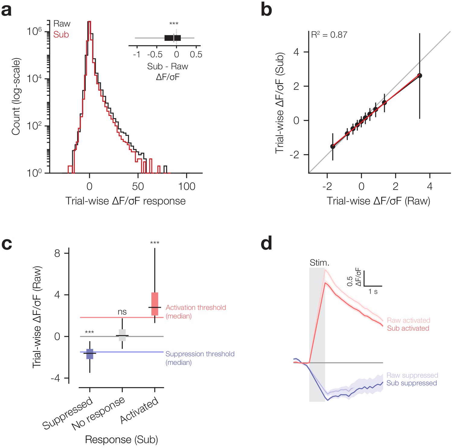
(a) Distribution of trial-wise responses on 50+ neuron stimulation trials calculated from raw (Raw; black) and neuropil subtracted (Sub; red) traces (N = 30,894 neurons, 1312 trials). A large fraction of negative responses are observed even in raw traces without neuropil subtraction. Inset: Difference between each neuron’s trial-wise response when responses were calculated from neuropil subtracted or raw traces (Sub – Raw). Responses are slightly reduced when traces are neuropil subtracted (−0.16 ± 0.58 ΔF/σF, p=0 Wilcoxon signed-rank test). (b) Neuropil-subtracted trial-wise responses are highly correlated with raw trial-wise responses (R2 = 0.87, p=0), although slightly reduced (β0 = -0.10 ± 5.32 x 10⁻⁴, p=0) with this reduction mainly limited to large positive going responses (β1 = 0.82 x 10⁻¹±3.31 × 10⁻⁴, p=0). Red: linear fit to data, Black: neuropil-subtracted data binned into deciles by raw trial-wise response and averaged within decile. Data are mean ± s.d. (c) Trial-wise responses classified as suppressed, activated and no response using neuropil-subtracted traces also show negative (−1.75 ± 1.05 ΔF/σF, p=0 Wilcoxon signed-rank test), roughly zero (0.16 ± 0.94 ΔF/σF, p=0, Wilcoxon signed-rank test) and positive (3.72 ± 3.18 ΔF/σF, p=0 Wilcoxon signed-rank test) trial-wise responses calculated from raw traces in the same trials. These groups also differed significantly from each other (p=0 Kruskal-Wallis test; Suppressed vs No response, p=0, Suppressed vs Activated, p=0, No response vs Activated, p=0, Bonferroni corrected for multiple comparisons) indicating that our thresholds on neuropil subtracted traces reliably separate different classes of trial-wise responses even in the absence of neuropil-subtraction. (d) Example raw (light red, light blue) and neuropil-subtracted (dark red, dark blue) traces for neurons reliably activated (red) and suppressed (blue) across trials (using neuropil-subtracted trial-wise magnitudes). Neuropil subtraction slightly decreases response magnitudes in both groups, though does not induce large changes in response time-course. Negative responses can be seen with and without neuropil-subtraction. Shading is mean ± s.e.m across neurons. Traces have been linearly interpolated across the photostimulation epoch (grey box) to avoid the photostimulation artefact for display only. All box-plots are median (mid-line) with 25th and 75th percentiles (box) and 5th and 95th percentiles (whiskers). N = 3.68 × 10⁶ trial-wise responses, 30894 neurons, 11 sessions, 6 mice, 1–2 sessions each.
Figure 3—figure supplement 3
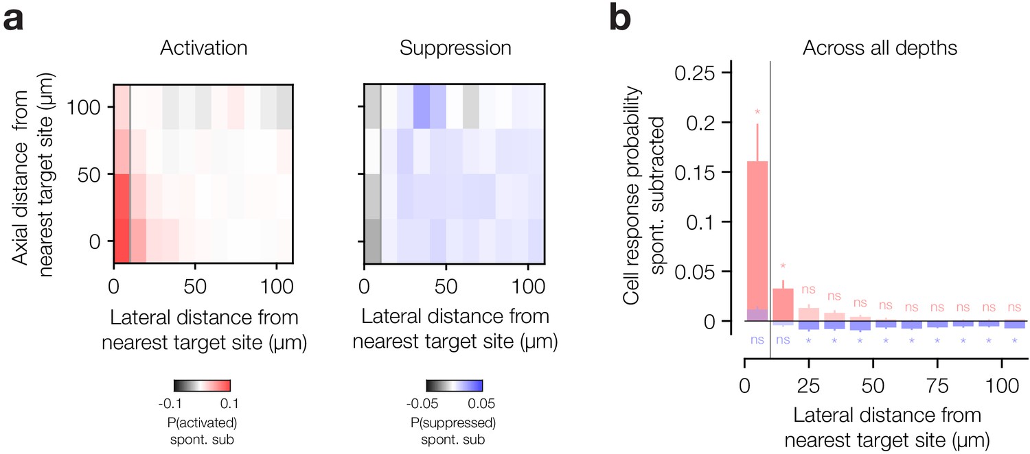
Activation and suppression have different spatial profiles.
(a) Lateral and axial spatial profile of activation (left) and suppression (right) relative to nearest target site co-ordinate: for each neuron plot its distance to nearest target site co-ordinate vs the proportion of trials it was activated or suppressed. Bin spatial distances and then average across all neurons in each bin. Average this value across stimulus trial types. (b) Quantification of spread of activation and suppression with lateral distance, collapsed across all axial planes. All data in all panels are hit:miss matched (see Figure 3—figure supplement 1 and Materials and methods) and have had catch trial values subtracted. All tests in (b) are Wilcoxon signed-rank tests, Bonferroni corrected for the number of lateral bins. * denotes p<0.05. N = 10 sessions, 6 mice, 1–2 sessions each. Note one session was excluded as there were no hits on catch trials so we were unable to subtract a hit:miss matched neural response rate on catch trials from the stimulus trial data. Error bars are s.e.m. and spatial bin widths are 10 µm.
Figure 4
Behaviour follows the activity of targeted ensembles despite matched suppression in the local network.
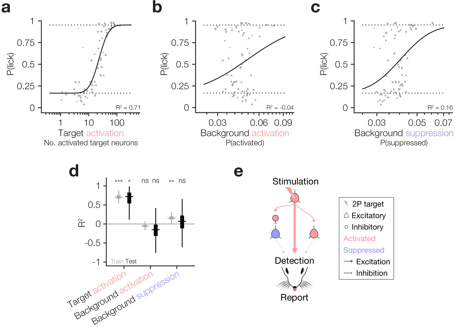
(a–c) Psychometric curve fits relating behavioural detection to the number of targets activated (a), the proportion of the background network activated (b) and the proportion of the background network suppressed (c). Solid lines: psychometric curve fit; dotted lines: fixed lapse rate (upper) and false alarm rate (bottom) for psychometric fit. Note that all neural data has been hit:miss matched (see Materials and methods) so the effective P(lick) for all datapoints is 0.5; however, for each datapoint we fit the actual recorded P(lick). The similarity of panel (a), which is hit:miss matched, to Figure 2d, which is not, demonstrates that the contribution of lick signals to the relationship between target activation and behaviour is negligible. Fits and R2 values reported are quantified on all data (compared to cross-validated fits in following panels). For these panels, N = 11 sessions, 6 mice, 1–2 sessions each. Some trial types from some sessions are excluded for having too few hits or misses to be able to match the hit:miss ratio. (d) Variance explained (R2) by the three predictors in (a–c) during the training (grey) and testing (black) phases of cross-validation (10,000 permutations of 80:20 train:test split). Only target activation strongly and reliably explains behaviour across both training and testing. Background suppression is mildly predictive of behaviour in model training datasets, but this relationship does not generalise to test datasets. Background activation does not explain behaviour. Boxplots are median with 25th and 75th percentile boxes and whiskers extending to the most extreme data points not considered outliers (see Materials and methods). (e) Schematic summarising the three tested routes from cortical activation to behavioural report highlighting that only the activity of target neurons has any reliable influence on behaviour despite matched suppression in the local network.
Additional files
Download links
A two-part list of links to download the article, or parts of the article, in various formats.
Downloads (link to download the article as PDF)
Open citations (links to open the citations from this article in various online reference manager services)
Cite this article (links to download the citations from this article in formats compatible with various reference manager tools)
How many neurons are sufficient for perception of cortical activity?
eLife 9:e58889.
https://doi.org/10.7554/eLife.58889


