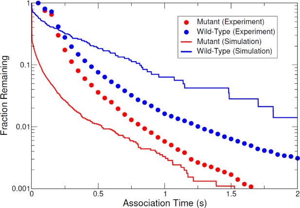
Cadherin clusters stabilized by a combination of specific and nonspecific cis-interactions
Figures
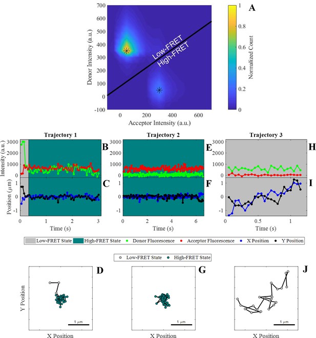
Observation of cis-interactions via single-molecule FRET.
(A) Representative heat map of donor and acceptor intensities showing two populations at high and low FRET efficiency indicated by the asterisks. The black line represents the threshold between the two states used to assign each observation to the high or low-FRET state. (B, E, H) Donor and acceptor trajectories for a FRET pair throughout representative trajectories, which are used to determine if the donor E-cad molecule is in a high-FRET or low-FRET state. (C, F, I) X and Y Cartesian coordinates for the donor or acceptor molecule over the length of the trajectory. (D, G, J) Two dimensional trajectory plots of the same trajectories, where the symbol color corresponds to the assigned FRET-state. The background of the trajectory time traces for intensity and position indicate the assigned FRET-state.

Heat maps showing binned acceptor and donor intensities using all molecular observations.
(A–C) Heat maps for the mutant and the intermediate and high concentration wild-type E-cad conditions, respectively. All heat maps show two distinct peaks corresponding to two populations (high-FRET/associated and low-FRET) indicated by the asterisks, where the black line is used to divide the two populations and assign each observation to either the high-FRET or low-FRET state. The low-FRET state is above the dividing line and the high-FRET state is below the dividing line.
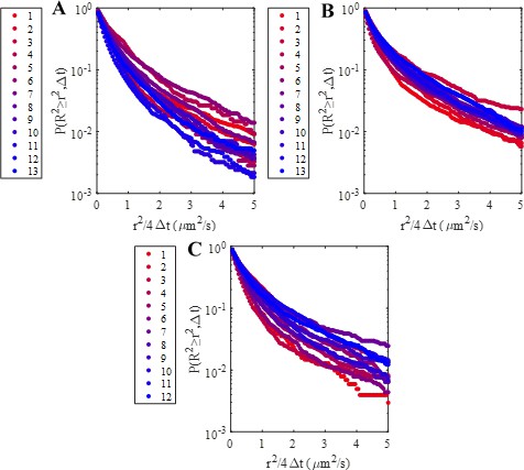
Overall complementary cumulative distributions of squared displacement calculated using only trajectories from a single movie for all three experimental conditions.
(A) High coverage wild-type, (B) intermediate coverage wild-type, and (C) high coverage mutant CCSDDs. Legends indicate the order of the movie that was used to calculate the CCSDD. No systematic trend in CCSDDs with sample imaging time (i.e. movie number) was observed.
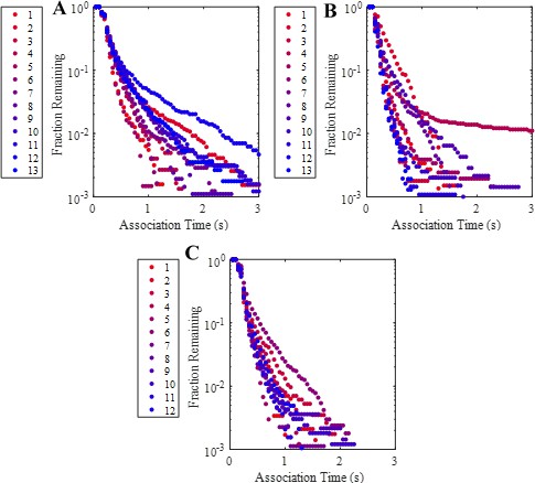
Complementary cumulative association time (high-FRET state dwell time) distributions calculated using only trajectories from a single movie for each of the three experimental conditions.
(A) High coverage wild-type, (B) intermediate coverage wild-type, and (C) high coverage mutant association time distributions. Legends indicate the order of the movie that was used to calculate the distributions. No systematic trend in distributions with sample imaging time (i.e. movie number) was observed.
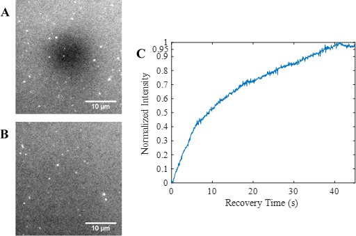
Fluorescence recovery after photobleaching (FRAP) analysis indicates the formation of a continuous, fluid supported lipid bilayer.
(A–B) Epifluorescence images showing the photobleached region 0 s and 40 s, respectively, after photobleaching. (C) FRAP recovery curve indicating a mobile fraction of greater than 0.95.
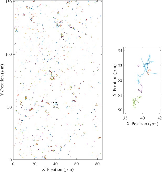
All localized and tracked trajectories two frames and longer from the 30 s high surface coverage wild-type movie clip included as Video 1 (left).
Zoomed in view of the region outlined by the dashed black square (right).
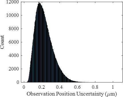
Representative histogram of positional localization uncertainties for all molecular observations for the high surface coverage wild-type condition indicating a significant number of observations with a large position uncertainty comparable to the size of a pixel (0.43 µm).
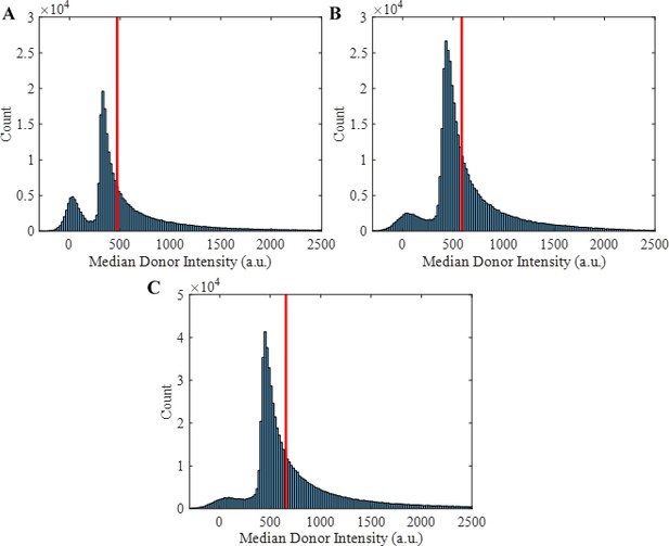
Trajectory median donor intensity histograms showing the 60th percentile cutoff as a vertical red line used to remove bright contaminants, donor E-cad aggregates, and donor E-cad labeled with multiple fluorophores.
The 60th percentile was selected as a consistent cutoff to remove trajectories corresponding to the tail of these distributions, as indicated by the figures. (A–C) Histograms for the mutant, high surface coverage wild-type, and intermediate surface coverage wild-type conditions, respectively.
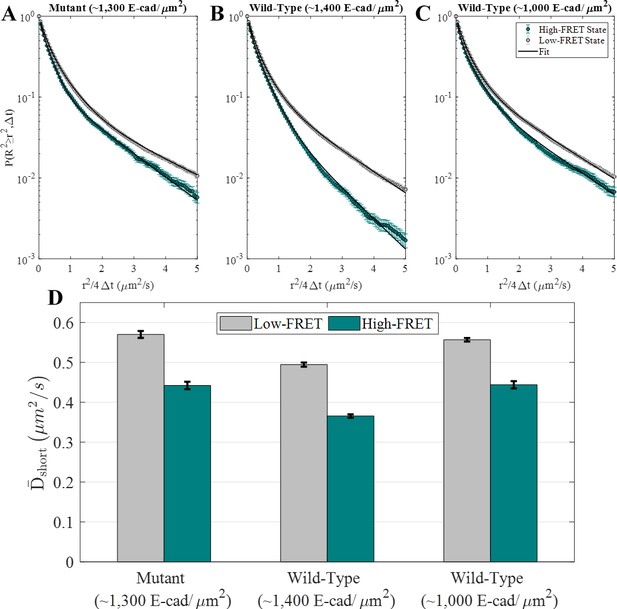
E-cad diffusion depends on FRET state and interaction capability.
(A–C) Complementary cumulative squared displacement distributions in the high-FRET and low-FRET states for the mutant and two wild-type E-cad conditions, along with the respective Gaussian mixture model fits. Error bars correspond to the standard deviation of CCSDDs calculated using 100 samples using a bootstrap method with replacement and are generally smaller than the data points, except in the ‘tail’ of the high-FRET state distributions. (D) in the high-FRET and low-FRET states for the mutant and two wild-type conditions. Error bars represent the standard deviation of fitting 100 samples using a bootstrap method with replacement.
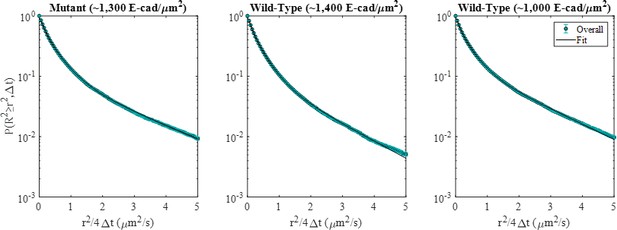
Overall CCSDDs, using all displacements from both high and low-FRET states, for the mutant and two wild-type E-cad conditions.
Gaussian mixture model fits are shown as the black curve. Error bars represent the standard deviation of 100 bootstrapped samples.
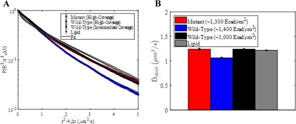
Displacement-based trajectory filtering results in short-time diffusion expected for supported lipid bilayers.
(A) Complementary cumulative squared displacement distributions for the three FRET conditions and a lipid in the bilayer. Solid black curves correspond to a two-term Gaussian mixture model fit. Trajectories shorter than 0.71 s or with a median single-frame displacement less than 0.3 µm were excluded from the analysis. Error bars correspond to the standard deviation of 100 distributions generated using a bootstrap sampling method. (B) Resulting values of the short-time diffusion coefficient calculated from the two-term Gaussian mixture model fitting. Error bars represent the standard deviation of short-time diffusion coefficients calculated by fitting 100 distributions generated using a bootstrap sampling method.
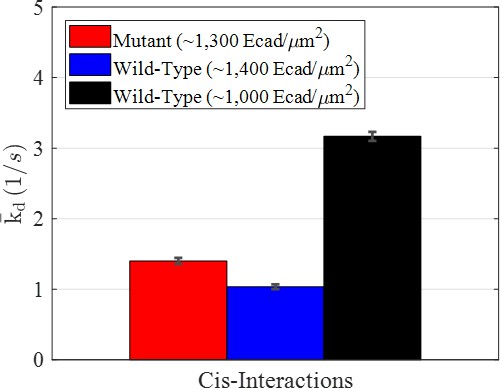
Average dissociation rate constants () for the mutant and two wild-type conditions resulting from modeling interactions using a Markov model.
Error bars were estimated as the square root of the Cramèr-Rao lower bound.
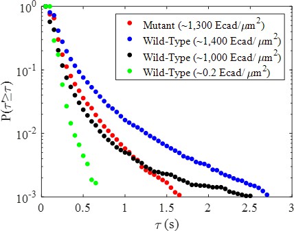
Complementary cumulative association time (high-FRET state dwell time) distributions calculated for each of the three high surface coverage experimental conditions and the low coverage control.
Notably, the low coverage control shows dramatically shorter dwell times than all other conditions.
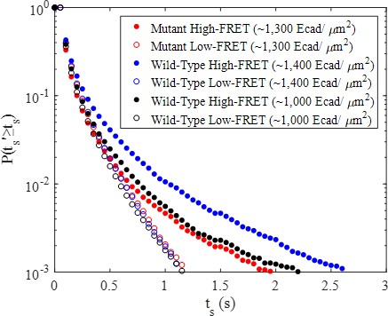
High-FRET and low-FRET complementary cumulative surface residence time (observation time) distributions for mutant E-cad and two concentrations of wild-type E-cad.
Qualitatively comparing the two wild-type high-FRET distributions indicates the probability of a long surface residence time increases with increasing surface coverage due to stronger lateral interactions.
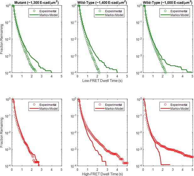
Complementary cumulative state dwell time distributions for the high and low-FRET states for the mutant and two wild-type E-cad conditions, compared to the predicted state dwell time distributions based upon the three-state, heterogeneous Markov model maximum likelihood estimate with beta-distributed transition probabilities.
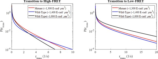
Probability density functions for the state transition rates between the high and low-FRET states for the mutant and wild-type conditions determined based upon the Markov model estimated, beta-distributed transition probabilities.
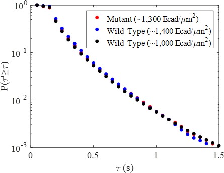
Low-FRET state complementary cumulative dwell time distributions for the mutant and two wild-type conditions.
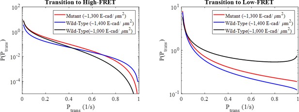
Beta distributions of state transition probabilities between the high and low-FRET states for the mutant and two wild-type conditions corresponding to the Markov model maximum likelihood estimated beta distribution parameters.
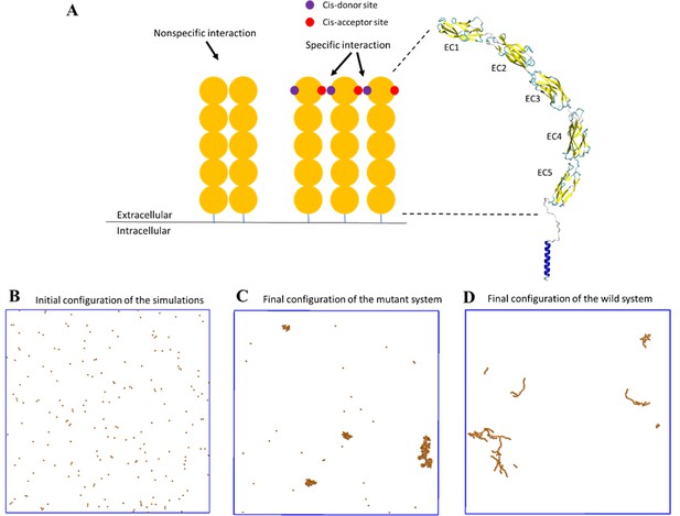
A coarse-grained model was constructed to simulate the spatial-temporal process of E-cad clustering.
(A) E-cad extracellular domains (orange), nonspecific and specific cis-interactions. Cis-donor sites are labeled in purple, and cis-acceptor sites are labeled in red. A structural model of the E-cad is shown on the right side. Ectodomain structure with EC domains 1–5 numbered from the N-terminus. (B) Top view of initial configuration in the simulations. The number of E-cad molecules is equal to 200. (C) Top view of final configuration in the mutant system. (D) Top view of final configuration in the wild-type system.
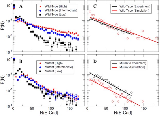
Specific and nonspecific interactions can cause E-cad clustering.
(A–B) Representative experimental cluster size probability distribution functions for wild-type and mutant E-cad at low, intermediate, and high surface coverages. Error bars correspond to the standard deviation of cluster size probability distribution functions calculated using 100 samples using a bootstrap method with replacement. (C–D) The comparison of experimental and simulated cluster size distributions for mutant and wild-type E-cad. The solid lines indicate the single exponential fitting.
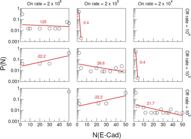
Distributions of mutant E-cad cluster size for different combinations of nonspecific interaction on/off rate.
The 1st, 2nd and 3rd columns correspond to on rate 2 × 10⁶ s−1, 2 × 10⁵ s−1, and 2 × 10⁴ s−1, respectively. The 1st, 2nd and 3rd rows correspond to off rate 104 s−1, 103 s−1, and 102 s−1, respectively. In each panel, the cluster size distributions are fitted by a single exponential function with a constant N0 corresponding to the characteristic cluster size. The fitted line and N0 values are colored in red.
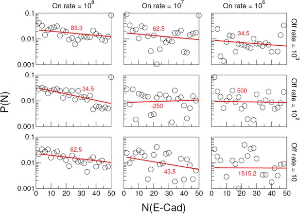
Distributions of wild-type E-cad cluster size for different combinations of specific interaction on/off rate.
The columns correspond to on rate 108 s−1, 107 s−1, and 106 s−1, respectively. The rows correspond to off rate 103 s−1, 102 s−1, and 10 s−1, respectively. Nonspecific interaction on and off rates, respectively, were fixed at 2 × 10⁵ s−1 and 103 s−1. In each panel, the cluster size distributions are fitted by a single exponential function with a constant N0 corresponding to the characteristic cluster size. The fitted line and N0 value are colored in red.
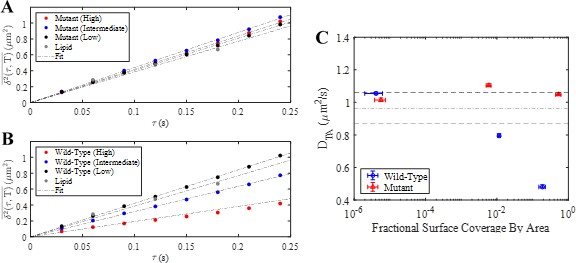
E-cad is primarily bound to a single lipid.
(A) Ensemble-time-averaged MSDs for mutant E-cad at high, intermediate and low surface coverage and a lipid in the bilayer. Linear fits are shown as the dot-dashed line. (B) Ensemble-time-averaged MSDs for wild-type E-cad at high, intermediate and low surface coverage and a lipid within the bilayer. Linear fits are shown as the dot-dashed line. (C) Resulting time-averaged diffusion coefficients (DTA) for wild-type and mutant E-cad as a function of fractional surface coverage by area. Error bars represent the 95% confidence interval calculated from fitting error. Fractional surface coverage by area calculations are described elsewhere by Thompson et al., 2019 (Thompson et al., 2019). The dot-dashed line represents the value of DTA for a lipid in an E-cad free bilayer and the dashed lines indicate the 95% confidence interval calculated from fitting error for the lipid MSD.
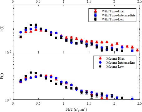
Trajectory averaged friction factor probability distributions for wild-type (top) and mutant (bottom) E-cad at high, intermediate, and low E-cad surface coverage.
The peak at a friction factor of ~0.5 s/µm2 corresponds to monomeric E-cad and was used to normalize all cluster size calculations.
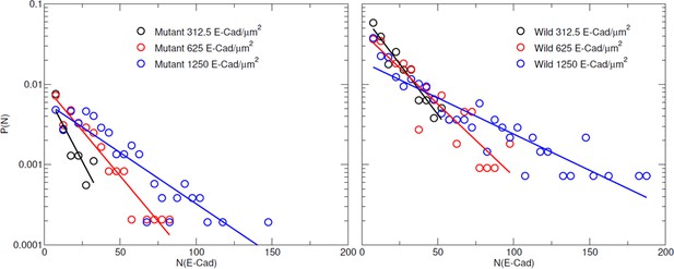
Distribution of cluster size for wild-type and mutant E-cad at a surface density of 312.5 E-cad/µm2, 625 E-cad/µm2, and 1,250 E-cad/µm2, respectively.
The data are fit to a single exponential.
Videos
High-coverage wild-type E-cad movie segment.
High-coverage mutant E-cad movie segment.
Intermediate-coverage wild-type E-cad movie segment.
Low-coverage wild-type E-cad control movie segment.
Lipid tracer control movie segment.
Tables
| Reagent type (species) or resource | Designation | Source or reference | Identifiers | Additional information |
|---|---|---|---|---|
| Cell line (human) | HEK293T | ATCC, Dr. Keith Johnson, University of Nebraska, Lincoln | CRL-3216 (RRID:CVCL_0063) | authenticated using STR-PCR and tested negative for mycoplasma |
| Transfected construct (human) | CEP 4.2 plasmid | Dr. Lawrence Shapiro, Columbia University | Encoding hexahistidine-tagged wild-type E-cad and L175D mutant | |
| Commercial assay or kit | Alexa Fluor 555 NHS-ester antibody labelling kit | Invitrogen | A20187 | Labeling E-cad |
| Commercial assay or kit | Alexa Fluor 647 NHS-ester antibody labelling kit | Invitrogen | A20186 | Labeling E-cad |
| Chemical compound, drug | DOPC | Sigma-Aldrich | P6354 | |
| Chemical compound, drug | DGS-NTA(Ni) | Avanti Polar Lipids | 790404 | |
| Chemical compound, drug | DOPE-LR | Avanti Polar Lipids | 810150 | |
| Software, algorithm | Custom Matlab-based software | 10.1021/acsmacrolett.8b00004; 10.1021/acsnano.8b02956; 10.1021/acs.jpclett.9b00004 | Image analysis | |
| Software, algorithm | simjFRAP | 10.1038/srep11655 | Image analysis |
Additional files
-
Supplementary file 1
Additional tables showing experimental parameters, simulation parameters, and sample size values.
- https://cdn.elifesciences.org/articles/59035/elife-59035-supp1-v2.docx
-
Transparent reporting form
- https://cdn.elifesciences.org/articles/59035/elife-59035-transrepform-v2.pdf


