Analysis of ultrasonic vocalizations from mice using computer vision and machine learning
- Laboratory of Physiology of Behavior, Department of Comparative Medicine, Yale School of Medicine, United States
- Institute of Informatics, Federal University of Rio Grande do Sul, Brazil
- Graduate Program in Biological Sciences - Biochemistry, Federal University of Rio Grande do Sul, Brazil
- Interdepartmental Neuroscience Program, Biological and Biomedical Sciences Program, Graduate School in Arts and Sciences, Yale University, United States
- Department of Neuroscience, Yale School of Medicine, Brazil
Figures
Figure 1 with 1 supplement
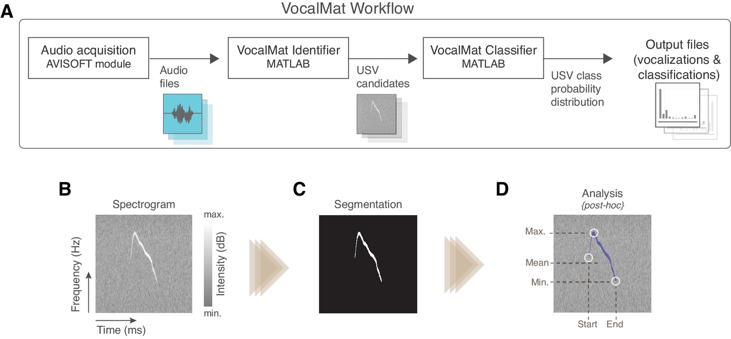
Overview of the VocalMat pipeline for ultrasonic vocalization (USV) detection and analysis.
(A) Workflow of the main steps used by VocalMat, from audio acquisition to data analysis. (B) Illustration of a segment of spectrogram. The time-frequency plan is depicted as a gray scale image wherein the pixel values correspond to intensity in decibels. (C) Example of segmented USV after contrast enhancement, adaptive thresholding, and morphological operations (see Figure 1—figure supplement 1 for further details of the segmentation process). (D) Illustration of some of the spectral information obtained from the segmentation. Information on intensity is kept for each time-frequency point along the segmented USV candidate.
Figure 1—figure supplement 1
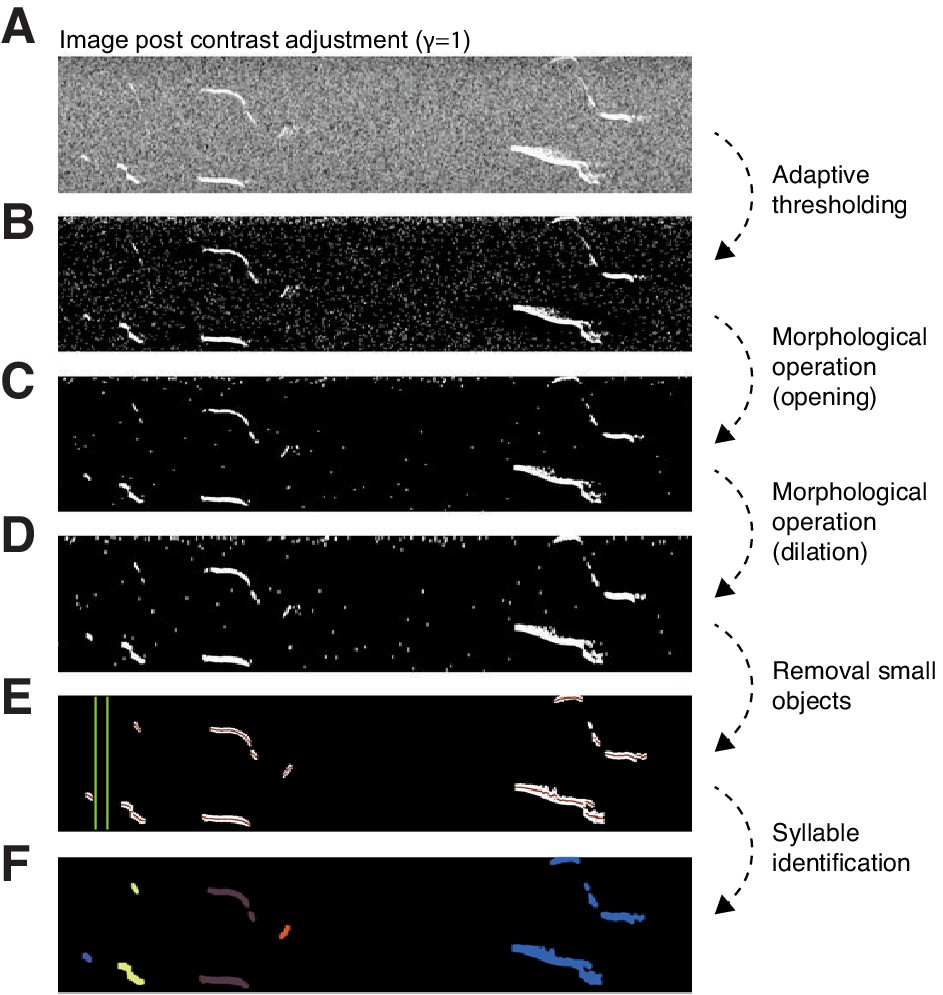
Image processing pipeline for segmentation of ultrasonic vocalizations (USVs) in spectrograms.
Image processing pipeline for segmentation of USVs in spectrograms. (A) Segment of a spectrogram post contrast adjustment (). (B) Output image post binarization using adaptive thresholding. (C) Resulting image from the opening operation with rectangle 4 × 2. (D) Result from the dilation with line l = 4 and 90°. (E) Removal of too small objects (≤60 pixels), mean of cloud points for each detected USV candidate being shown in red and green lines shows an interval of 10 ms. (F) Result after separating syllables based on the criterion of maximum interval between two tones in a syllable. The different colors differentiate the syllables from each other.
Figure 2
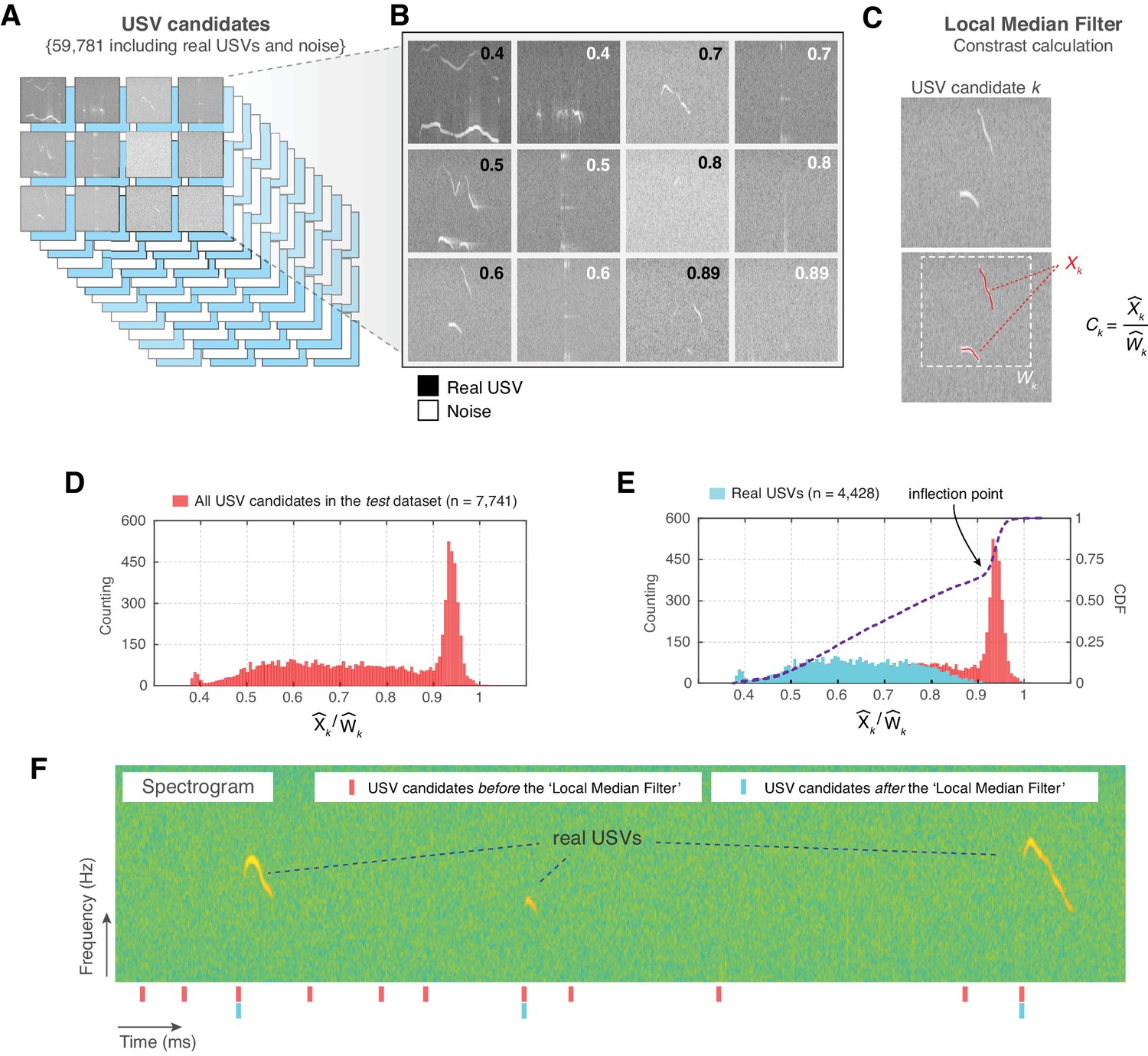
Noise elimination process for ultrasonic vocalization (USV) candidates.
(A) In a set of 64 audio files, VocalMat identified 59,781 USV candidates. (B) Examples of USVs among the pool of candidates that were manually labeled as either noise or real USVs. The score (upper-right corner) indicates the calculated contrast for the candidate. (C) Example of contrast calculation ( ) for a given USV candidate . The red dots indicate the points detected as part of the USV candidate () and the dashed-white rectangle indicates its evaluated neighborhood (). (D) Distribution of the for the USV candidates in the test data set. (E) Each USV candidate was manually labeled as real USV or noise. The distribution of for the real USVs (cyan) compared to the distribution for all the USV candidates (red) in the test data set. The blue line indicates the cumulative distribution function (CDF) of for all the USV candidates. The inflection point of the CDF curve is indicated by the arrow. (F) Example of a segment of spectrogram with three USVs. The analysis of this segment without the ’Local Median Filter’ results in an elevated number of false positives (noise detected as USV). ’Red’ and ’cyan’ ticks denote the time stamp of the identified USV candidates without and with the ’Local Median Filter’, respectively.
Figure 3
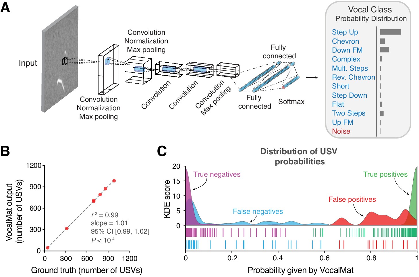
VocalMat ultrasonic vocalization (USV) classification using a convolutional neural network.
(A) Illustration of the AlexNet architecture post end-to-end training on our training data set. The last three layers of the network were replaced in order to perform a 12-categories (11 USV types plus noise) classification task. The output of the CNN is a probability distribution over the labels for each input image. (B) Linear regression between the number of USVs manually detected versus the number reported by VocalMat for the audio files in our test data set (see Figure 4—figure supplement 1 for individual confusion matrices). (C) Distribution of probabilities for the true positive (green), false positive (red), false negative (cyan), and true negative (magenta). Ticks represent individual USV candidates.
Figure 4 with 1 supplement

VocalMat performance for ultrasonic vocalization (USV) classification.
(A) Example of the 11 categories of USVs plus noise that VocalMat used to classify the USV candidates. (B) Confusion matrix illustrating VocalMat’s performance in multiclass classification (see also Supplementary file 5 and Figure 4—figure supplement 1 for individual confusion matrices). (C) Comparison of classification performance for labels assigned based on the most likely label (Top-one) versus the two most likely labels (Top-two) (see Supplementary file 6). Symbols represent median ±95% confidence intervals.
Figure 4—figure supplement 1
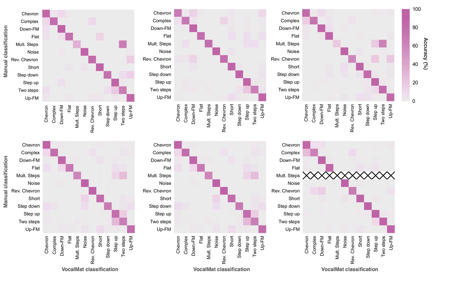
Confusion matrix illustrating VocalMat’s performance in multiclass classification per recording file.
Figure 5 with 1 supplement
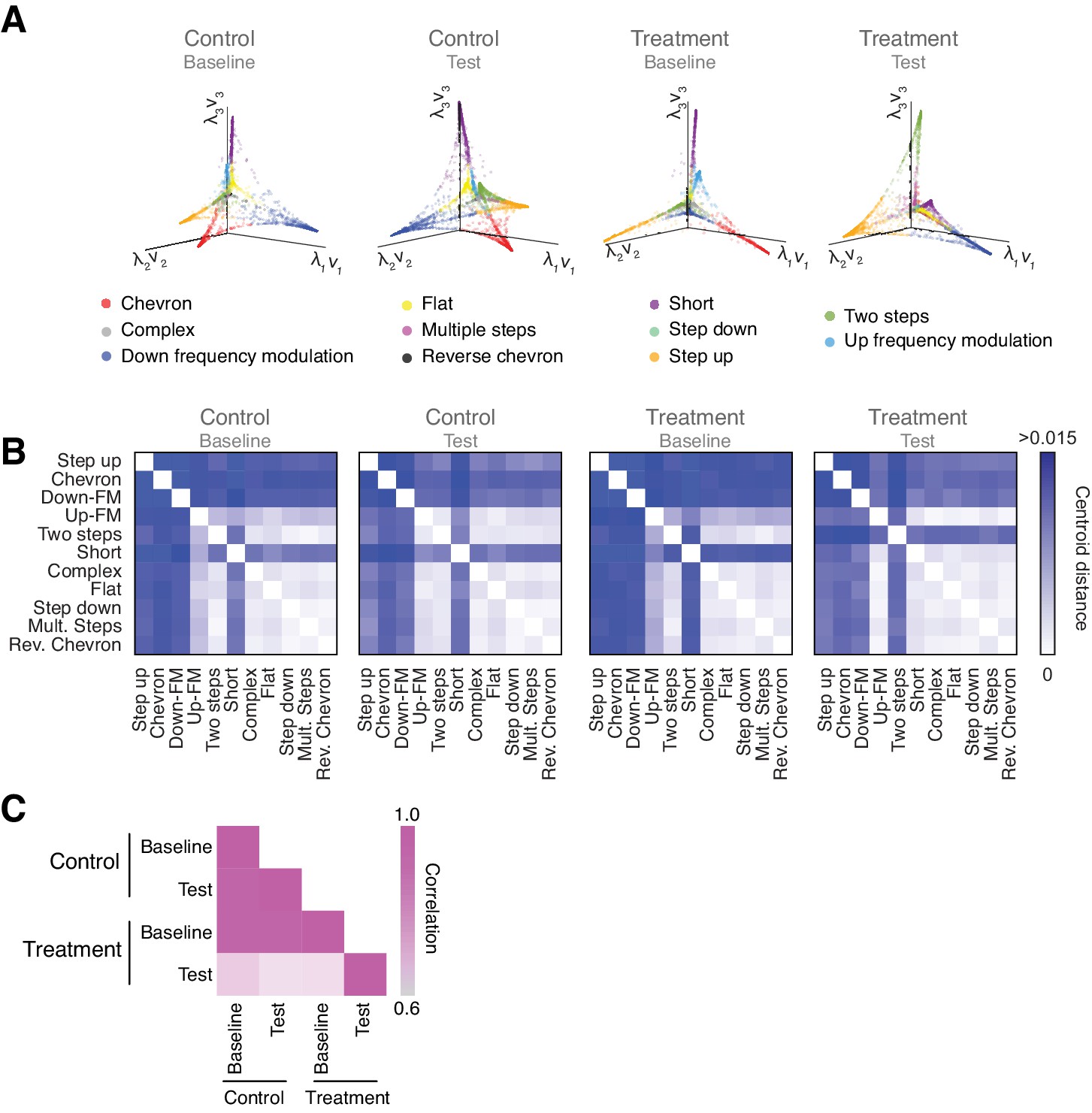
Vocal repertoire visualization using Diffusion Maps.
(A) Illustration of the embedding of the ultrasonic vocalizations (USVs) for each experimental condition. The probability distribution of all the USVs in each experimental condition is embedded in a Euclidean space given by the eigenvectors computed through Diffusion Maps. Colors identify the different USV types. (B) Pairwise distance matrix between the centroids of USV types within each manifold obtained for the four experimental conditions. (C) Comparison between the pairwise distance matrices in the four experimental conditions by Pearson’s correlation coefficient.
Figure 5—figure supplement 1
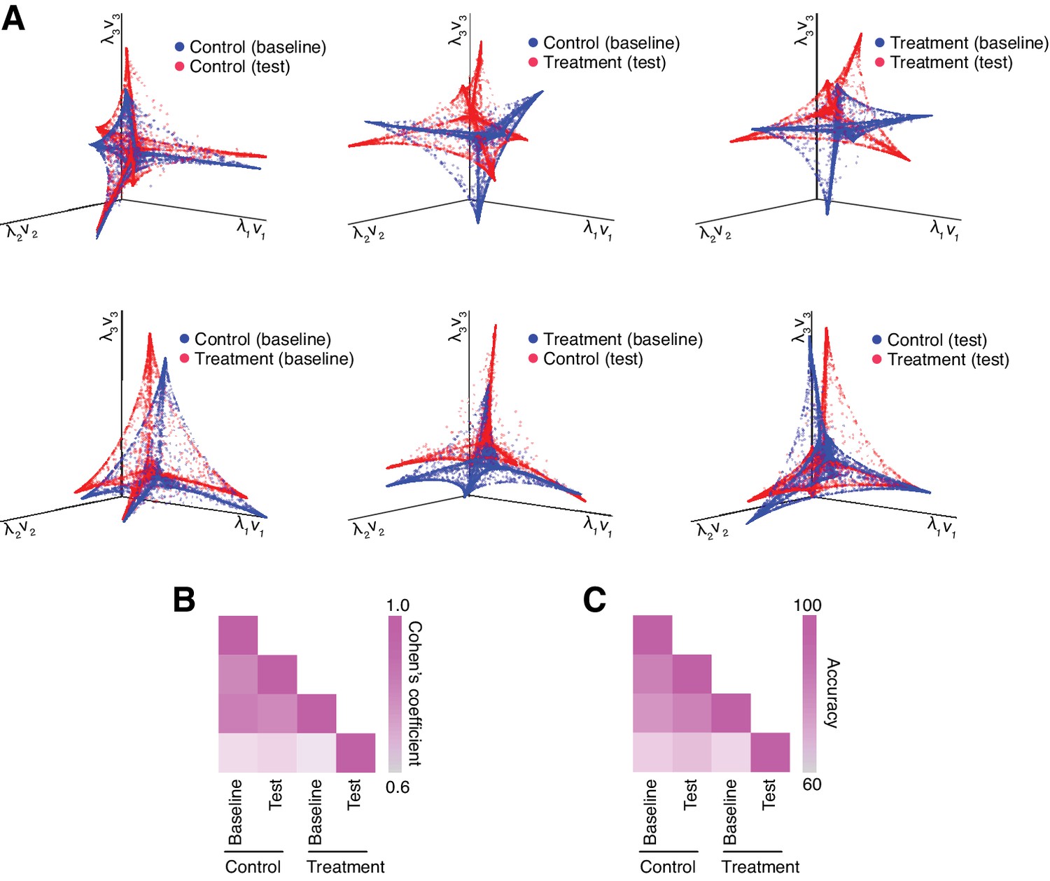
Alignment of the manifolds between pairs of experimental conditions.
(A) Illustration of the resulting manifold alignment for each pair of experimental conditions. The quality of the alignment between the manifolds is assessed by (B) Cohen’s coefficient and (C) overall projection accuracy into joint space.
Tables
Table 1
Summary of performance of VocalMat in detecting ultrasonic vocalizations (USVs) in the test data set.
| Audio file | True positive | False negative | True negative | False positive | Accuracy (%) |
|---|---|---|---|---|---|
| 1 | 316 | 1 | 58 | 2 | 99.20 |
| 2 | 985 | 1 | 105 | 15 | 98.55 |
| 3 | 696 | 12 | 73 | 5 | 97.84 |
| 4 | 862 | 13 | 51 | 4 | 98.17 |
| 5 | 44 | 1 | 216 | 3 | 98.48 |
| 6 | 696 | 2 | 87 | 4 | 99.24 |
| 7 | 787 | 5 | 122 | 5 | 98.91 |
Table 2
Summary of detection performance.
| Tool | Missed ultrasonic vocalizations (USVs) rate (%) | False discovery rate (%) |
|---|---|---|
| Ax | 4.99 | 37.67 |
| MUPET | 33.74 | 38.78 |
| USVSEG | 6.53 | 7.58 |
| DeepSqueak | 27.13 | 7.61 |
| VocalMat | 1.64 | 0.05 |
Table 3
Summary of experimental conditions covered in the test data set.
| Age | Microphone gain | Location | Heating |
|---|---|---|---|
| P9 | Maximum | Environmental chamber | No |
| P9 | Maximum | Environmental chamber | No |
| P9 | Maximum | Environmental chamber | No |
| P10 | Intermediary | Open field | No |
| P10 | Intermediary | Open field | No |
| P10 | Maximum | Environmental chamber | Yes |
| P10 | Maximum | Environmental chamber | Yes |
Additional files
-
Supplementary file 1
List of parameters and performance of Ax.
- https://cdn.elifesciences.org/articles/59161/elife-59161-supp1-v2.docx
-
Supplementary file 2
List of parameters and performance for MUPET.
- https://cdn.elifesciences.org/articles/59161/elife-59161-supp2-v2.docx
-
Supplementary file 3
List of parameters and performance for USVSEG.
- https://cdn.elifesciences.org/articles/59161/elife-59161-supp3-v2.docx
-
Supplementary file 4
List of parameters and performance for DeepSqueak.
- https://cdn.elifesciences.org/articles/59161/elife-59161-supp4-v2.docx
-
Supplementary file 5
VocalMat accuracy per class.
- https://cdn.elifesciences.org/articles/59161/elife-59161-supp5-v2.docx
-
Supplementary file 6
VocalMat accuracy considering the two most likely labels.
- https://cdn.elifesciences.org/articles/59161/elife-59161-supp6-v2.docx
-
Transparent reporting form
- https://cdn.elifesciences.org/articles/59161/elife-59161-transrepform-v2.docx
Download links
A two-part list of links to download the article, or parts of the article, in various formats.
Downloads (link to download the article as PDF)
Open citations (links to open the citations from this article in various online reference manager services)
Cite this article (links to download the citations from this article in formats compatible with various reference manager tools)
Analysis of ultrasonic vocalizations from mice using computer vision and machine learning
eLife 10:e59161.
https://doi.org/10.7554/eLife.59161


