3DeeCellTracker, a deep learning-based pipeline for segmenting and tracking cells in 3D time lapse images
- Graduate School of Science, Nagoya City University, Japan
- Department of Biological Sciences, Graduate School of Science, Osaka University, Japan
- Departments of Biomedical Engineering and Radiology and the Zuckerman Mind Brain Behavior Institute, Columbia University, United States
- Graduate School of Information Science and Technology, Hokkaido University, Japan
- National Institute for Physiological Sciences, Japan
- Exploratory Research Center on Life and Living Systems, Japan
- National Institute for Basic Biology, National Institutes of Natural Sciences, Japan
- The Graduate School for Advanced Study, Japan
- Department of Biology, Faculty of Science, Kyushu University, Japan
- RIKEN center for Advanced Intelligence Project, Japan
Figures
Figure 1 with 2 supplements
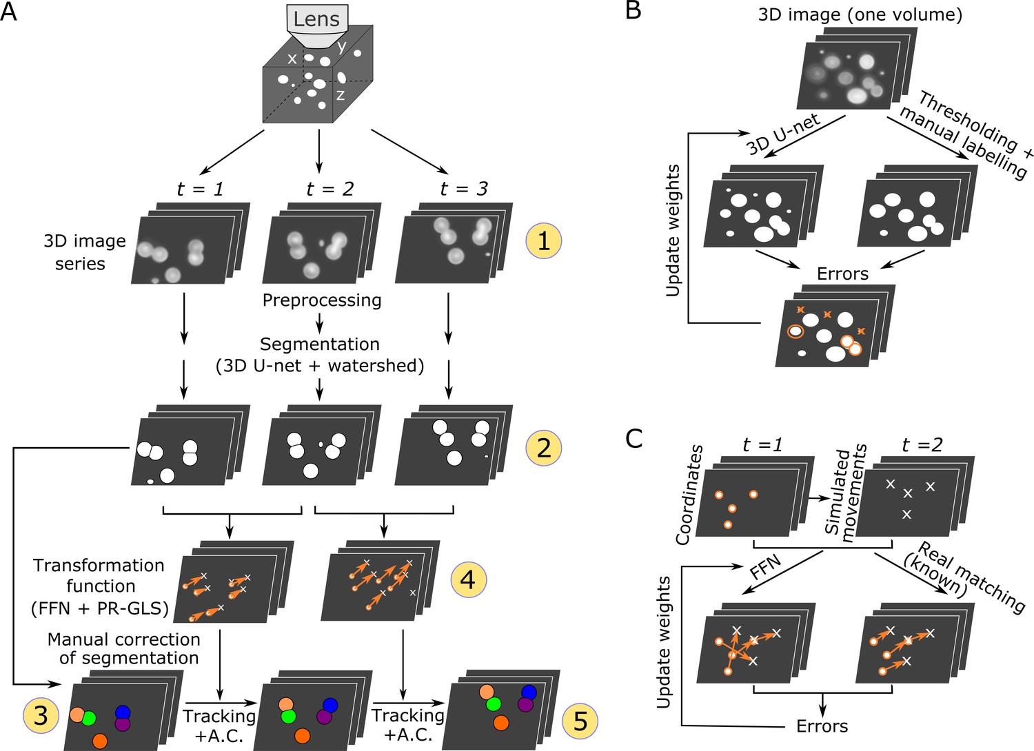
Overall procedures of our tracking method and the training procedures of the deep networks.
(A) Procedures of segmentation and tracking. 3D + T images are taken as a series of 2D images at different z levels (step 1) and are preprocessed and segmented into discrete cell regions (step 2). The first volume (t = 1) of the segmentation is manually corrected (step 3). In the following volumes (t ≥ 2), by applying the inferred transformation functions generated by FFN + PR-GLS (step 4), the positions of the manually confirmed cells are successively updated by tracking followed by accurate corrections (A.C.) (step 5). The circled numbers indicate the five different procedure steps. (B) Procedures for training the 3D U-net. The cell-like regions predicted by 3D U-net are compared with manually labeled cell regions. The errors (orange) are used to update U-net weights. (C) Procedures for training the feedforward network. The movements of cells used for training are generated from simulations, thus their correct matches are known. The errors in the predictions are used to update the feedforward network weights.
Figure 1—figure supplement 1

Illustration of segmentation and tracking.
Cell nuclei labeled with a fluorescent protein are scanned into 3D + T images and segmented into individual nuclei. The positions of segmented nuclei varied over time due to organ movement and/or deformation. These nuclei are tracked by updating their positions.
Figure 1—figure supplement 2

Illustration of the visual inspection of the tracking results.
The tracking results were compared with the raw images in each volume visually to find tracking mistakes.
Figure 2 with 4 supplements
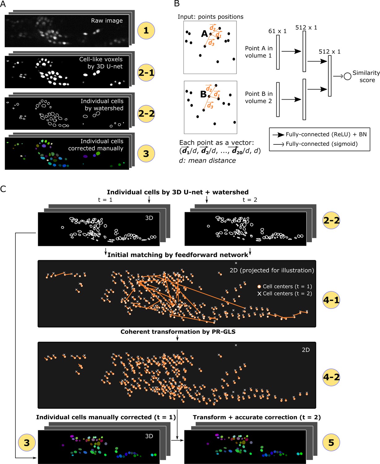
Detailed descriptions of segmentation and tracking.
(A) Details of segmentation. The circled numbers correspond to the numbers in Figure 1, while the numbers 2–1 and 2–2 indicate cell-like voxels detected by 3D U-net and individual cells segmented by watershed, respectively. One volume of a worm neuron dataset is used as an example. (B) Left: Definition of the positions in two point sets corresponding to two volumes. Right: Structure of the feedforward network for calculating the similarity score between two points in two volumes. The numbers on each layer indicate the shape of the layer. ReLU: Rectified linear unit. BN: Batch normalization. (C) Details of tracking. 4–1 and 4–2 indicate the initial matching from t = 1 to t = 2 using our custom feedforward network and the more coherent transformation function inferred by PR-GLS, respectively. The orange lines in 4–1 and 4–2 indicate the inferred matching/transformation from t = 1 to t = 2.
Figure 2—figure supplement 1

Structures of the 3D U-Net used in this study.
We designed different structures for adopting different resolutions of images, which is preferred but not necessary. End-users can freely choose one of the structures for their own data for simplicity. (A) Used for datasets worm #1 and #2, and for the binned zebrafish dataset. (B) Used for dataset worm #3 and the degenerated worm datasets. (C) Used for the raw zebrafish dataset. Each raw 3D image was split into sub-images and then sent into the network as input (top left) to generate maps of cell regions as output (top right), finally these maps for sub-images were combined. In the network, images were filtered and compressed to lower-resolution then recovered to the original resolution again, in order to utilize both local and global features. Numbers on each intermediate layer indicate the number of convolutional filters, while numbers on the left of each row indicate the size of the 3D images of input, output, and intermediate layers. Conv: Convolution; BN: Batch normalization.
Figure 2—figure supplement 2

Illustration of the FFN training method.
(A) Generation of the synthetic data for training the FFN. The locations of a point set (orange circles) were transformed by affine function with different parameters, and additional movements of the transformed points were incorporated by adding random movements to each point. (B) The matching by FFN between two test point sets, which was improved in accuracy over the course of training.
Figure 2—figure supplement 3

Comparison of our method with previous tracking techniques.
(A and B) Comparison of the initial matchings made by FPFH (Rusu et al., 2009) and FNN. Cell centers were generated from the 3D U-net + watershed segmentation of two volumes in worm #3 dataset. Blue dots indicate cell centers, and orange lines indicate the estimated matches between these two point sets. We manually counted the error rates. In the regular process, matching is between temporally adjacent volumes. In this panel, we performed matching between the points separated for 10 volumes (t1 and t2) as an example of a challenging condition. (C) The predicted positions from the three methods (affine alignment, FPFH + PR-GLS, and FFN + PR-GLS) and the real positions of cells at t2. (D) The distances between the predicted positions and their real positions for the three methods.
Figure 2—figure supplement 4

Illustration of the accurate correction.
(A and B) Our method for accurately correcting cell locations. (A) Correction method in the single cell case. We obtained the region (the large solid black ellipse) and the center (small black circle) of a cell predicted by PR-GLS from the previous volume. We also obtained cell regions detected by 3D U-Net (the dashed blue ellipse). Subsequently, we calculated the intersection of the PR-GLS region and 3D U-Net regions (filled with diagonal blue lines) and its center (small blue circle). The final accurate correction follows the small black arrow, that is the center of the cell should move from the small black circle to the small blue circle. (B) Correction method when two regions predicted by PR-GLS partially overlapped. The method is essentially the same as in (A), except that areas where two PR-GLS regions overlapped were removed from the intersection region of PR-GLS and 3D U-net, generating two smaller regions (diagonal blue lines). We used this technique to prevent the two cells from merging in tracking results. (C) An example of accurate correction with a worm neuron dataset. The locations of the cells predicted by FFN + PR-GLS (middle) had small discrepancies with their real positions in the raw image (top). Such discrepancies were corrected (white arrows) by our method (bottom). All panels are correspoinding to a 2D layer of a 3D image at z = 66.
Figure 3 with 6 supplements
Results for dataset worm #1a.
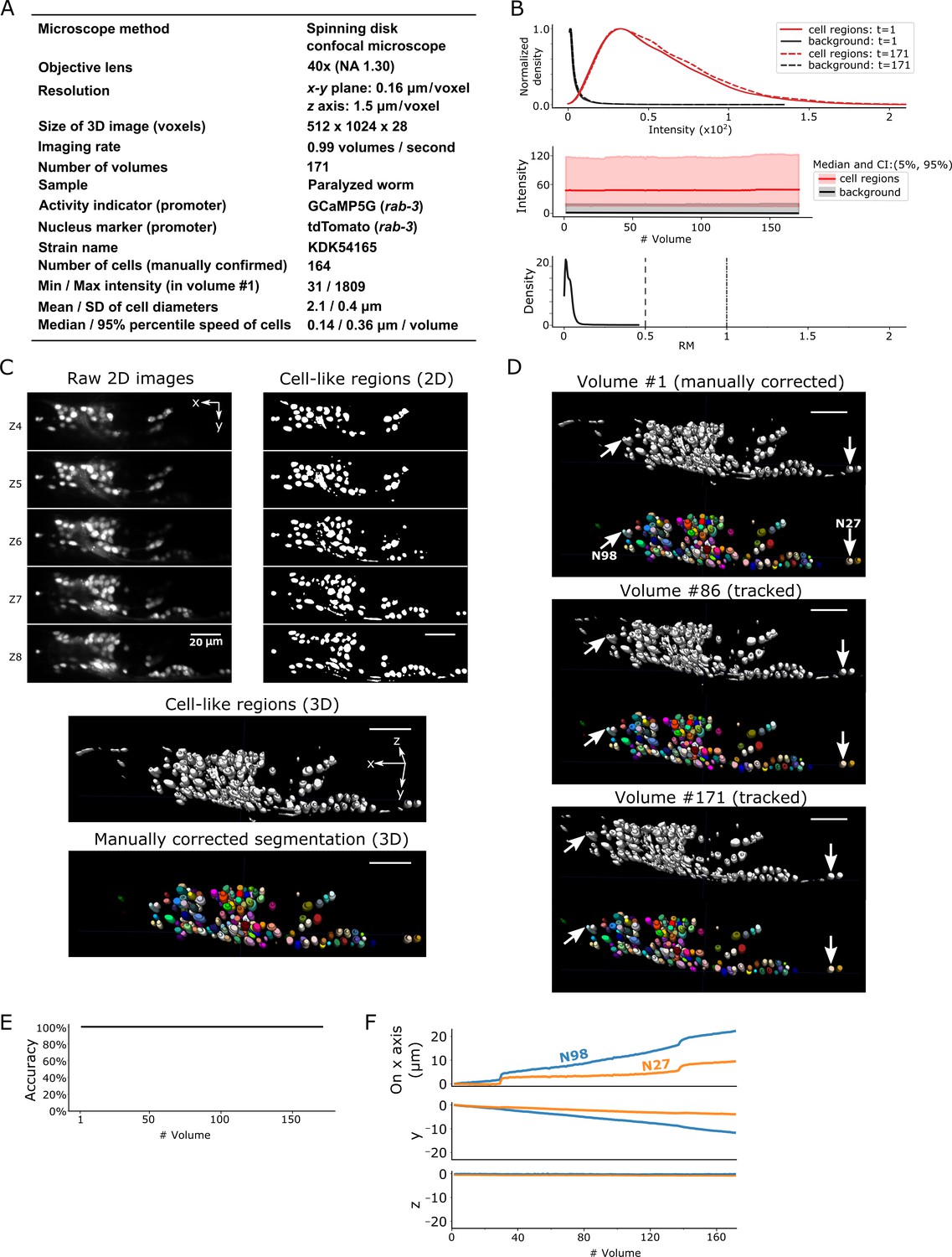
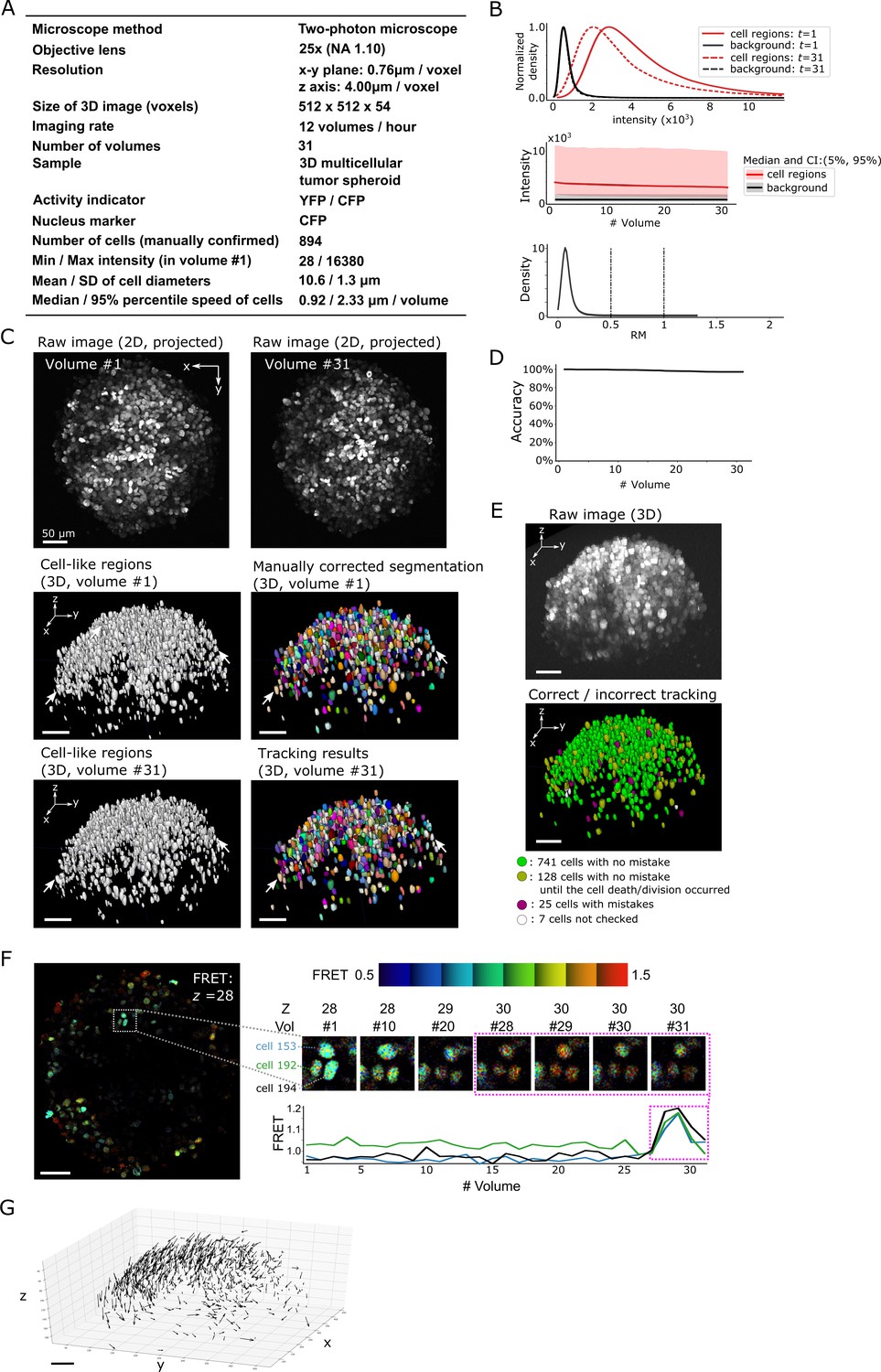
(A) Experimental conditions. (B) The distribution (top) and the time-course changes (middle) of the intensities in cell regions and in the background, and the distribution of relative movements (bottom). The distributions were estimated using the ‘KernelDensity’ function in Scikit-learn library in Python. The intensities were calculated using 8-bit images transformed from the 16-bit raw images. The relative movement (RM) is the normalized cell movement: RM = movement/(distance to the closest cell). The critical values, RM = 0.5 and 1.0, are emphasized by dashed and dash-dotted lines, respectively (see Figure 4 and Materials and methods for details). CI: confidence interval. (C) 3D image and its segmentation result in volume #1. Top left: Five layers (Z4–Z8) of the raw 2D images. Top right: Cell-like regions corresponding to the 2D images at left, detected by the 3D U-Net. Middle: Cell-like regions of the 3D view including all layers. Bottom: Final segmentations using watershed plus manual correction. Different colors represent different cells. (D) Tracking results. Tracked cells in volume #86 and volume #171 are shown, which are transformed from the segmentation in volume #1. In each panel, the top shows the cell-like regions detected by 3D U-Net, and the bottom shows tracked cells. Arrows indicate two example cells with large (N98) and small movement (N27). All cells were correctly tracked. (E) The tracking accuracy through time. (F) Movements of the two representative cells N98 and N27 in x, y, and z axes, indicating an expansion of the worm mainly in the x-y plane. The initial positions at volume #1 were set to zero for comparison. All scale bars, 20 µm.
Figure 3—figure supplement 1
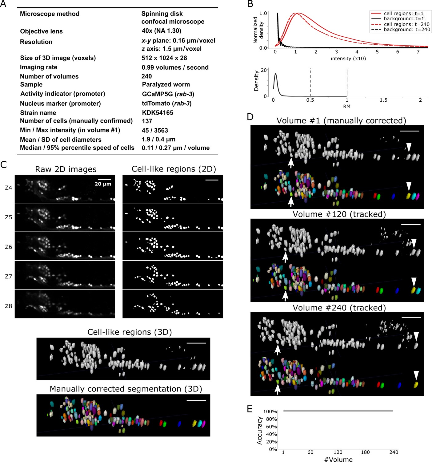
Results for dataset worm #1b.
(A) Experimental conditions. (B) Intensities and movements. (C) 3D image and its segmentation result in volume #1. (D) Tracking results. Tracked cells in volume #120 and volume #240 are shown. Arrows and arrowheads indicate two tracked cells. All the cells were correctly tracked except for those that moved out of the field of view of the camera. (E) Tracking accuracy through time. All scale bars, 20 µm.
Figure 3—figure supplement 2

Results for dataset worm #2.
(A) Experimental conditions. (B) Intensities and movements. (C) 3D image and its segmentation result in volume #1. (D) Tracking results. Tracked cells in volume #19 and #36 are shown. Arrows and arrowheads indicate two tracked cells. All cells were correctly tracked. (E) Tracking accuracy through time. (F) Movements of the two representative cells N29 and N99. When compared with Figure 3F, these cells showed small but irregular movements in the x-y plane. All scale bars, 20 µm.
Figure 3—figure supplement 3

Results for dataset worm #3.
(A) Experimental conditions. (B) Intensities and movements. (C) 3D image and its segmentation result in volume #1. (D) Tracking results. The tracked cells in volume #275 and #591 are shown. Arrows and arrowheads indicate two tracked cells. For their movements, see Figure 9L. Only four neurons were mistracked. (E) Tracking accuracy through time. (F) The positions of cells with/without tracking mistakes. Some small cells are invisible. All scale bars, 20 µm.
Figure 3—video 1
Tracking results for dataset worm #1a.
The animation of cell regions (top) detected by 3D U-net and corresponding individual cells (bottom) in dataset #1a tracked by our method.
Figure 3—video 2
Tracking results for dataset worm #2.
The animation of cell regions (top) detected by 3D U-net and corresponding individual cells (bottom) in dataset #2 tracked by our method.
Figure 3—video 3
Tracking results for dataset worm #3.
The animation of cell regions (top) detected by 3D U-net and corresponding individual cells (bottom) in dataset #3 tracked by our method.
Figure 4
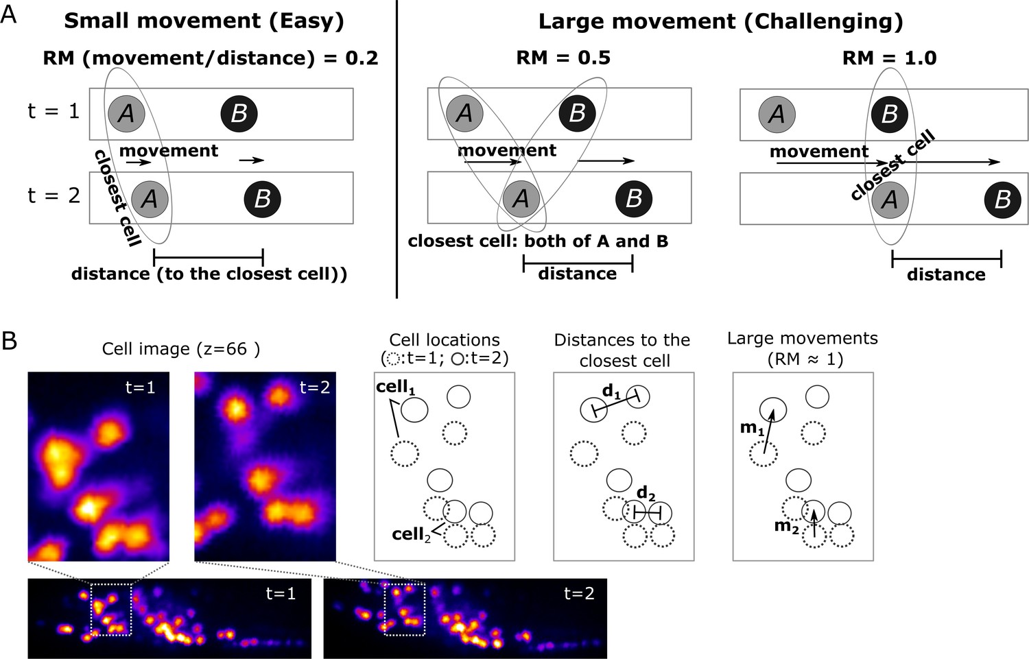
Quantitative evaluation of the challenging relative movement (RM) of cells.
(A) Illustrations of movements in one dimensional space with RM = 0.2, 0.5, and 1.0. Here RM = (movement a cell traveled per volume)/(distance to the closest neighboring cell). When RM ≥0.5, cell A at t = 2 will be incorrectly assigned to cell B at t = 1 if we simply search for its closest cell instead of considering the spatial relationship between cells A and B. When RM = 0.5, cell assignment is also impossible. Please also see Materials and methods for details. (B) Examples of large cell movements with RM ≈ 1. Also see Figure 10 and Table 3.
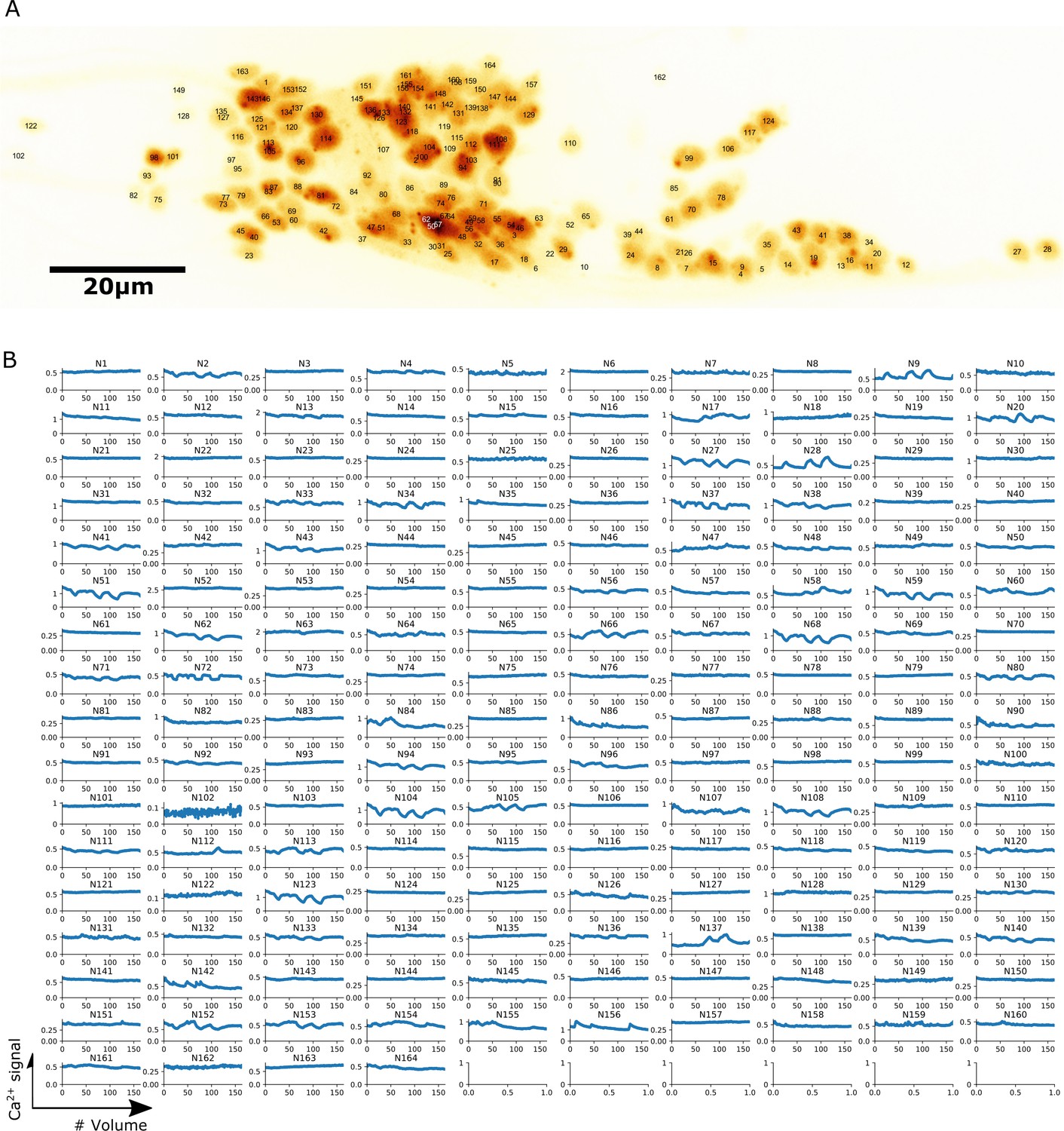
Figure 5 with 3 supplements

Localization and calcium dynamics in all 137 neurons for dataset worm #1b.
(A) The ID numbers of neurons were superimposed on the image of cell nuclei (tdTomato) projected onto the 2D plane. The orientation of the image has been rotated to align the anterior-posterior axis with the horizontal direction. To increase the visibility of both nuclei and IDs, we inverted the intensity of the nuclei image and displayed it using the pseudocolor ‘glow’. (B) Extracted calcium dynamics (GCaMP / tdTomato) in all 137 neurons. All cells were correctly tracked, while some of them moved out of the field of the camera and thus their activities were recorded for shorter periods.
Figure 5—figure supplement 1
Localization and calcium dynamics in all 164 neurons for dataset worm #1a.
(A) The ID numbers of neurons were superimposed on the image of cell nuclei (tdTomato) projected onto the 2D plane. (B) Extracted activities (GCaMP/tdTomato) in all 164 neurons.
Figure 5—video 1
GCaMP signals in dataset worm #1a.
The dynamics and movements of GCaMP signals in dataset #1a projected onto the 2D plane. The intensity was displayed using the pseudocolor ‘fire’.
Figure 5—video 2
GCaMP signals in dataset worm #2.
The dynamics and movements of GCaMP signals in dataset #2 projected onto the 2D plane.
Figure 6 with 1 supplement
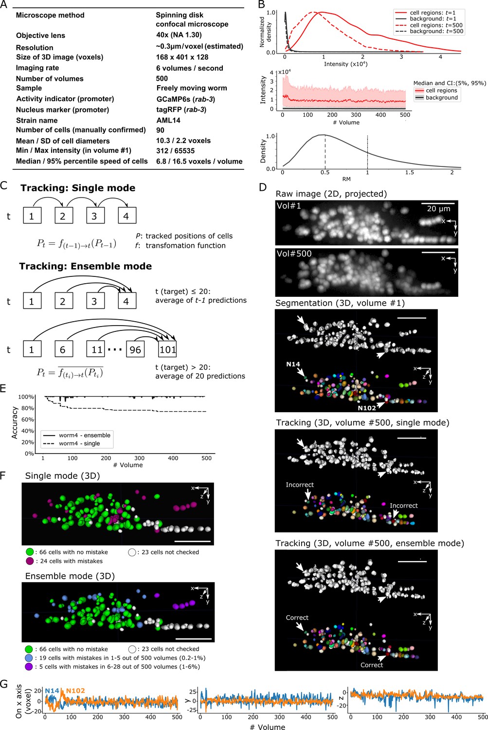
Results for dataset worm #4 – ‘straightened’ freely moving worm.
(A) Experimental conditions. (B) Intensities and movements. (C) The two methods (single mode and ensemble mode) we used for tracking this dataset. (D) The results of segmentation and tracking using the two methods. The intensity of the raw images (top) was enhanced for the visibility (adjusted ‘gamma’ value from 1 to 0.5). (E) The tracking accuracy through time. (F) The positions of 90 cells with/without tracking mistakes in the single (top) and ensemble (bottom) modes. (G) Movements of the two representative cells N14 and N102 in x, y, and z axes. All scale bars, 20 µm.
Figure 6—video 1
Tracking results for the ‘straightened’ freely moving dataset worm #4.
The animation of cell regions (top) detected by 3D U-net and corresponding individual cells (bottom) in dataset #3 tracked by our method in ensemble mode.
Figure 7 with 3 supplements
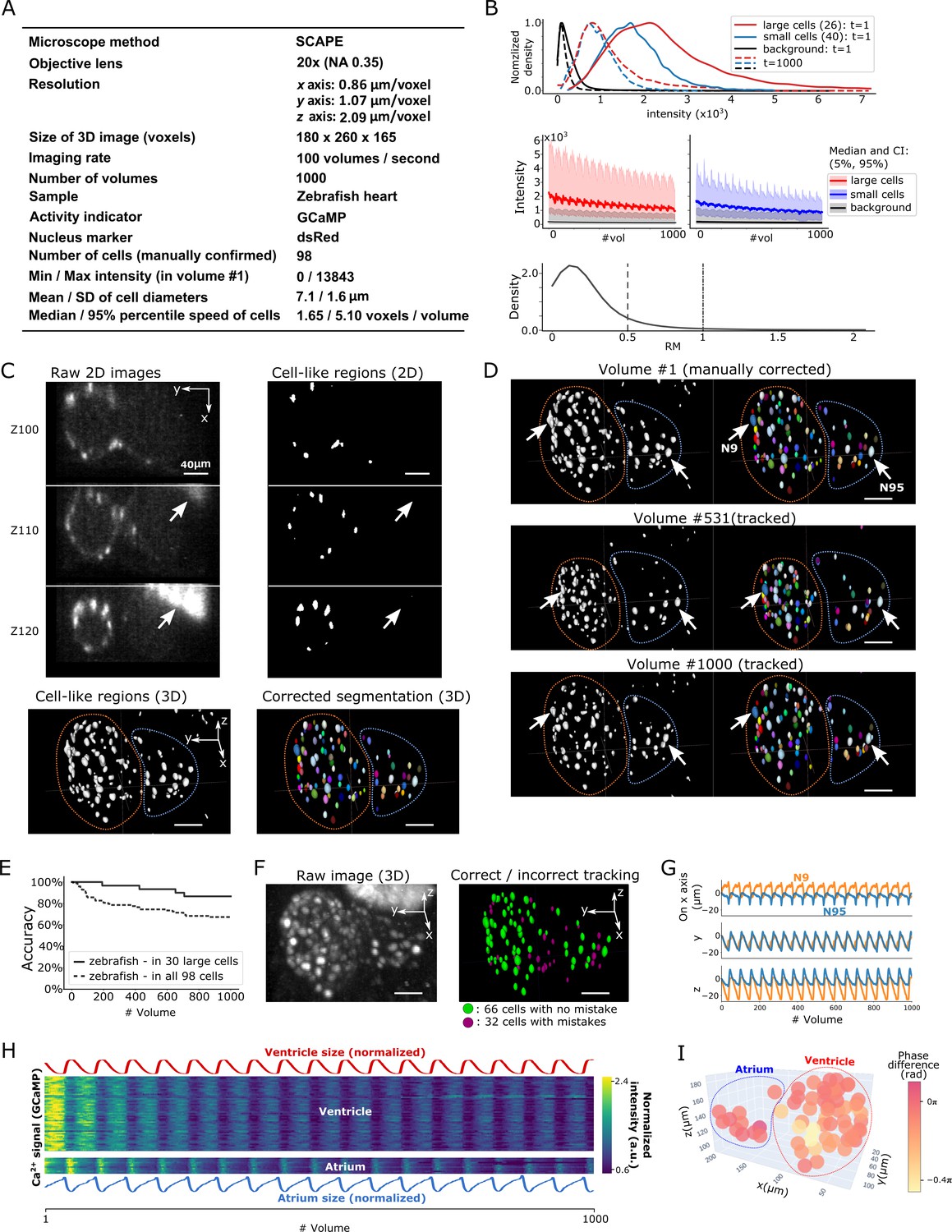
Results from tracking beating cardiac cells in zebrafish.
(A) Experimental conditions. (B) Intensities and movements of the correctly tracked cells with large size (26 cells) or small size (40 cells). (C) 2D and 3D images and its segmentation result in volume #1. The large bright areas in Z110 and Z120 indicated by arrows are irrelevant for the tracking task, and our 3D U-net correctly classified them as background. Orange and blue outlines in bottom panels indicate the regions of the ventricle and atrium, respectively. (D) Tracking results. Tracked cells in volume #531 and #1000 are shown; we showed #531 because #500 looks similar to #1. Arrows indicate two correctly tracked representative cells in the ventricle and atrium. The sizes of the ventricle and atrium changed periodically (orange and blue outlines). (E) Tracking accuracy in 30 large cells or in all 98 cells through time. (F) The positions of 98 cells with/without tracking mistakes. (G) Movements of the two representative cells N9 and N95, indicating regular oscillations of cells in whole 3D space. (H) Dynamics of ventricle size, atrium size, and calcium signals in ventricle cells and atrium cells. The sizes of the ventricle and atrium cannot be directly measured, so we instead estimated them as , where sd is standard deviation (more robust than range of x, y, z), and x, y, z are coordinates of correctly tracked cells in the ventricle or in the atrium. To improve visibility, these sizes were normalized by . Calcium signals (GCaMP) were also normalized by . (I) Phase differences between intracellular calcium dynamics and the reciprocal of segment sizes in ventricle and atrium were estimated. Here we used reciprocal of segment sizes because we observed the anti-synchronization relationships in (H). The phase differences were estimated using cross-correlation as a lag with the largest correlation. Most cells showed similar phase differences (mean = −0.110 π; standard deviation = 0.106 π). All scale bars, 40 µm.
Figure 7—figure supplement 1
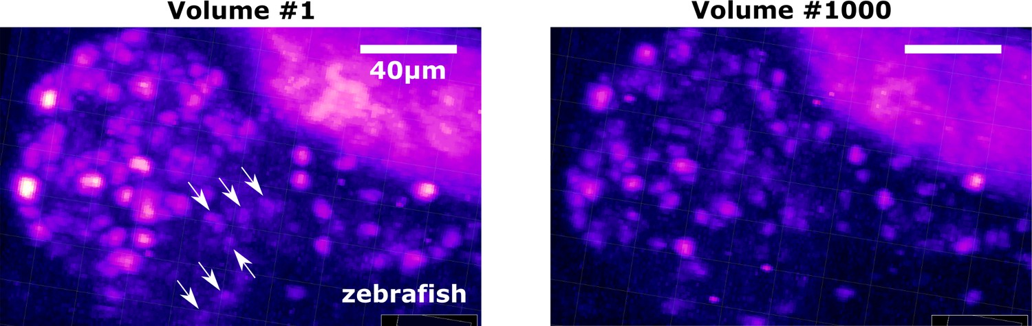
Examples of cells with weak intensities and photobleaching in the zebrafish dataset.
All cells were visualized in 3D view. The left and right images are displayed under the same brightness/contrast setting; the right image (Volume #1000) was much darker than the left image (Volume #1) due to photobleaching. Arrows: example cells with weaker intensities that were more difficult to segment and track than the stronger ones. All scale bars, 40 µm.
Figure 7—video 1
dsRed signals in the zebrafish dataset.
The intensity and movements of cell nuclei (dsRed) in the zebrafish dataset projected onto the 2D plane. The intensity of nuclei changed due to contraction and expansion of cells during beating.
Figure 7—video 2
Tracking results of the zebrafish dataset.
The animation of beating cardiac cell regions (left) detected by 3D U-net and corresponding individual cells (right) in the zebrafish dataset tracked by our method.
Figure 8 with 2 supplements
Results from tracking the cells in a 3D tumor spheroid.
(A) Experimental conditions. (B) Intensities and movements. (C) Raw 2D images (top), cell-like regions (middle left and bottom left), segmented cells in volume #1 (middle right) and the tracking result in volume #31 (bottom right). (D) Tracking accuracy through time with a small decrease from 100% (volume #1) to 97% (volume 31). (E) The positions of cells with/without tracking mistakes. Seven cells (white) were not checked because segmentation mistakes were found in volume #1 in these cells during the confirmation of tracking. (F) An example of the extracted activity (FRET = YFP/CFP). Left: one layer of the FRET image at z = 28 in volume #1. The movements and intensities of three cells in the square are shown on the right side. The extracted activities of the three cells are shown in the graph. (G) Movements of the 741 cells that experienced neither tracking mistakes nor cell death/division. Arrows indicate the location changes from volume #1 to #31. All scale bars, 50 µm.
Figure 8—video 1
CFP signals in the tumor spheroid dataset.
The intensity and movements of cell nuclei (CFP) in the tumor spheroid dataset (3D view).
Figure 8—video 2
Tracking results of the tumor spheroid dataset.
Upper: The cell regions detected by 3D U-net. Lower: Individual cells tracked by our method.
Figure 9 with 2 supplements
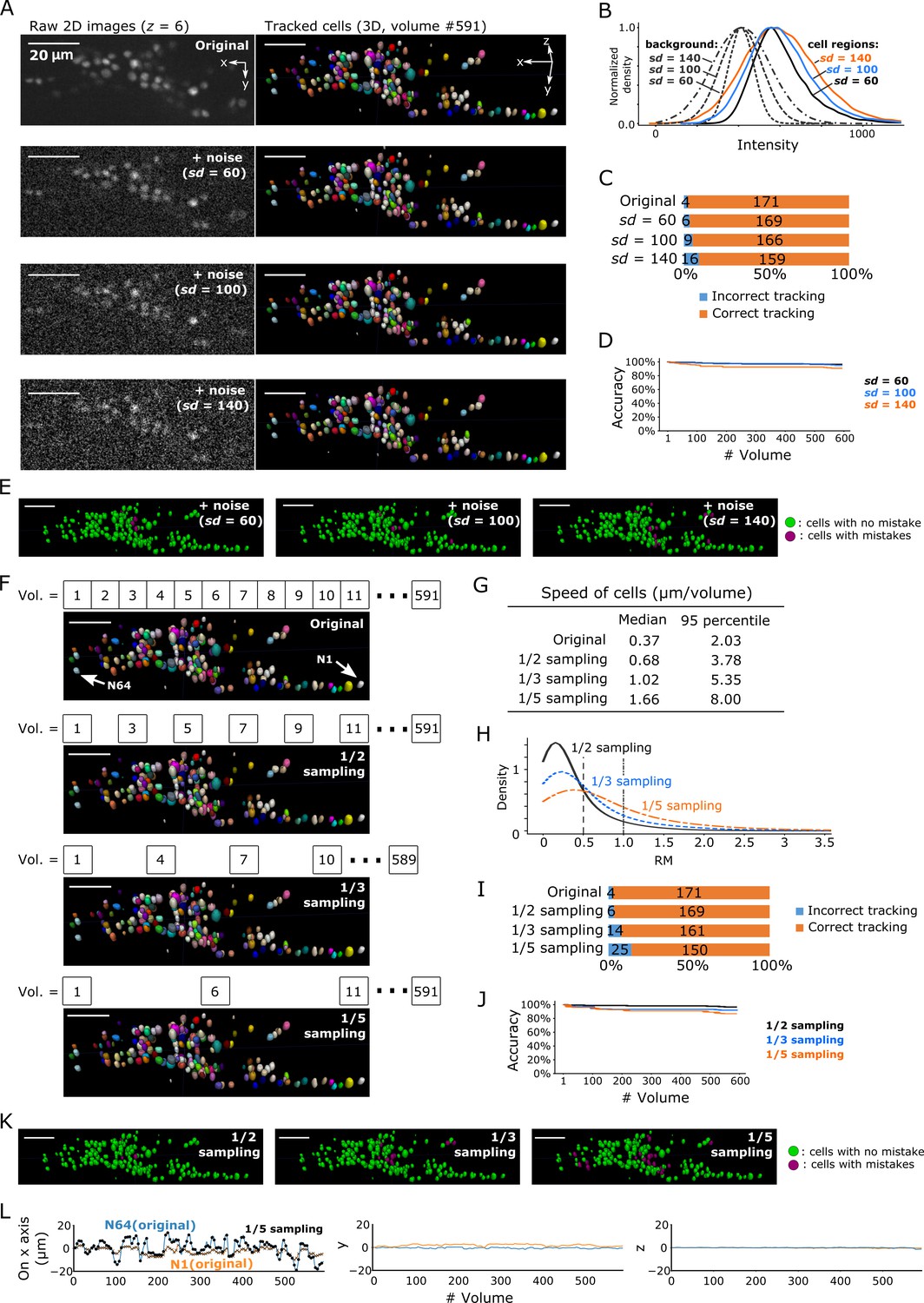
Robustness of our method in artificially generated challenging conditions.
(A) Tracking results when Poisson noise was added to dataset worm #3. One layer (z = 6) of 2D images (left, volume #1) and the corresponding tracking results in the last volume were shown (right). (B) Distributions of intensities of cell regions (solid lines) and background (dashed lines) from images with added noise. All distribution curves were normalized so that their peaks have the same height. (C) Bar graph showing the numbers of incorrectly tracked and correctly tracked cells for the four noise levels. (D) Tracking accuracies of the datasets with added noise through time. (E) The positions of cells with/without tracking mistakes. The numbers of cells with correct/incorrect tracking are shown in panel C. (F) Tracking results in the last volume when sampling rates were reduced by removing intermediate volumes in dataset worm #3. Arrows indicate two representative cells. (G) Statistics of cell speed based on the tracking results of the 171 correctly tracked cells in the original images. The speeds in 1/5 sampling conditions are much larger than in the original conditions, which makes the cells more challenging to track. (H) Distributions of movements. (I) Bar graph showing the numbers of incorrectly tracked and correctly tracked cells for the four sampling rates. (J) Tracking accuracies of the downsampled datasets through time. (K) The positions of cells with/without tracking mistakes. The numbers of cells with correct/incorrect tracking are shown in panel I. (L) Movements of the two representative cells N64 and N1, indicating iterative expansion and contraction of the worm mainly in the x-axis. The movements between neighboring volumes after applying 1/5 sampling (black dots and crosses) are larger than the movements in the original dataset worm #3 (blue and orange lines). See Figure 3—figure supplement 3 and Figure 3—video 3 for tracking results in the original dataset worm #3. All scale bars, 20 µm.
Figure 9—figure supplement 1
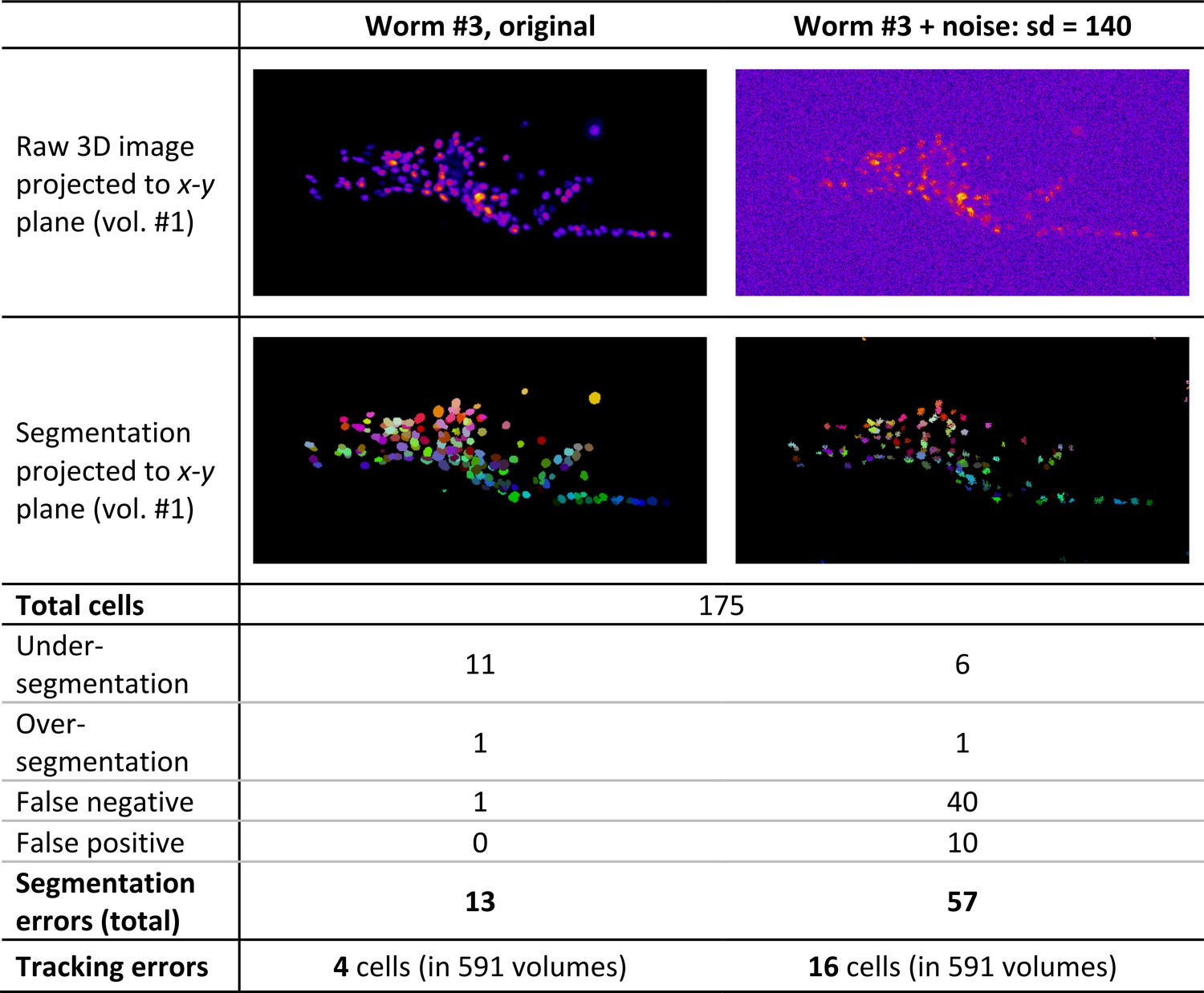
Errors in segmentation and tracking in two example image datasets.
Numbers of the cells that were incorrectly segmented (in volume #1) and incorrectly tracked (in any volume) are shown. We manually checked the segmentation errors in two images. Compared to the number of segmentation errors (13 and 57), the number of tracking errors are much lower (4 and 16), implying that most incorrectly segmented cells were still correctly tracked. Note that segmentation errors were manually corrected in vol #1 but not in the following volumes.
Figure 9—figure supplement 2
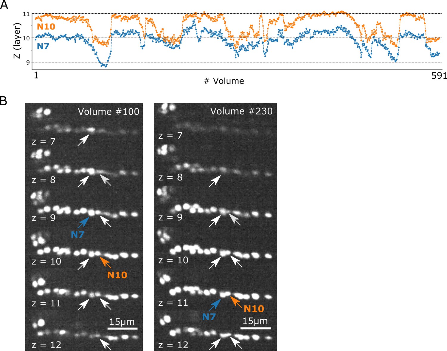
Cross-layer movements of two cells.
(A) Examples of cross-layer movements of two cells in dataset worm #3. The positions of the centroids of each cell (z) were calculated as the average locations of the segmented regions corresponding to that cell. (B) The positions of the two cells (arrows) and their centroids (blue and orange) in raw images at volumes #100 and #230.
Figure 10 with 2 supplements
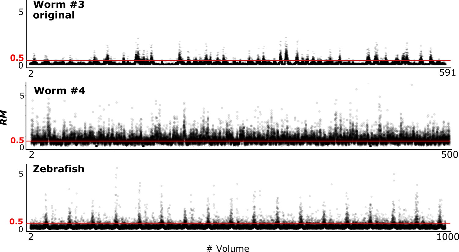
RM values at different time points in three datasets.
Figure 10—figure supplement 1

The relationship between movements and the error rate of our method.
(A) The relationship in the real datasets. (B) The relationship in the downsampled worm #3 datasets. The RM is the averaged RM in each volume. The error rate is the number of new errors divided by the number of correctly tracked cells until the last volume. We fitted regression lines using the kernel ridge regression with RBF kernel. The top and right parts show the marginal distributions of RM and error rate, respectively.
Figure 10—figure supplement 2
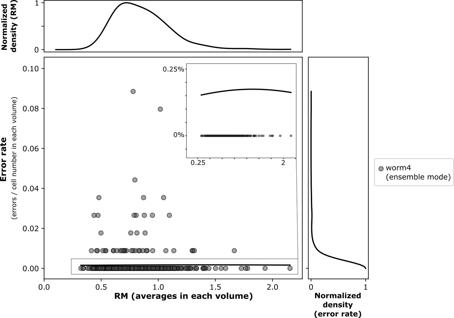
The relationship between movements and the error rate of our method in ensemble mode.
The result is based on the freely moving worm dataset (worm #4).
Figure 11 with 2 supplements

Comparison of the tracking results between our method, DeepCell 2.0, and Toyoshima et al., 2016.
(A) Comparison with DeepCell 2.0 tested using the layer z = 9 in worm #3. The raw images (top) are displayed using the pseudocolor ‘fire’. Colors in the tracking results (middle and bottom) indicate the initial positions (volume #1, left) and tracked positions of cells (volume #519, right). Note that the spatial patterns of cell colors in the initial and last volumes are similar in our method (middle) but not in DeepCell 2.0 (bottom). Arrows indicate all the correctly tracked cells in our method and in DeepCell 2.0. Cells without arrows were mistracked. The asterisk indicates a cell whose centroid moved to the neighboring layer (z = 10) and thus was not included in the evaluation. Also see Figure 11—video 1 and Table 4. (B) Comparison with Toyoshima’s software tested using all layers in worm #3 with 1/5 sampling rate. For demonstration, we only show tracking results at z = 9. Again arrows indicate all the correctly tracked cells in our method and in Toyoshima’s software. Because Toyoshima’s software is not able to label the tracked cells using different colors, all cells here are shown by purple circles. Some cells were not marked by circles because they were too far from the centroids of the cells (in other layers). See also Table 4. All scale bars, 20 µm.
Figure 11—figure supplement 1

Comparision of the tracking accuracies between our method and two previous methods.
(A) Tracking accuracies by DeepCell 2.0 and by our method for two 2D image datasets. (B) Tracking accuracies by Toyoshima et al., 2016 and by our method for three 3D image datasets. For the zebrafish dataset, Toyoshima ‘s method showed low accuracy from the first volume because of segmentation errors.
Figure 11—video 1
Tracking results of a 2D + T image (z = 9 of worm #3) using our method and DeepCell 2.0.
The tracked cells are shown in different colors. In our method, most cells were correctly tracked and their colors did not change (top). In DeepCell 2.0, most cells were incorrectly tracked and their colors changed during the tracking (bottom).
Tables
Table 1
Comparison between the complexities of our method and a previous method.
For each method, the procedures are listed along with the number of parameters (in bold) to be manually determined by researcher (see the guide in our GitHub repository). Our method requires manual determination of less than half of the parameters required by the previous method.
| Our method | Toyoshima et al., 2016 | |||
|---|---|---|---|---|
| Procedures | Parameters | Procedures | Parameters | |
| Pre-processing | Alignment | - | Alignment | - |
| Local contrast normalization | (1) Noise level | Denoising (median filter) | (1) Radius | |
| Background subtraction | (2) Radius | |||
| Gaussian blurring | (3) Radius | |||
| Segmentation | 3D U-net (detect cell/non-cell regions) | Automatically learned | Thresholding | (4) Method (e.g., ‘mean’,’ triangle’) |
| Watershed 1 | (5) Radius (6) Minimum size of cells | |||
| Watershed (twice) | (2) Minimum size of cells | Counting number of negative curvature | (7) Threshold (8) Distance to borders | |
| Watershed 2 | - | |||
| Tracking | Feedforward network (generate an initial matching) | Automatically learned | Least squares fitting of Gaussian mixture | (9-11) Default value of covariance matrix (3d vector) |
| PR-GLS (generate a coherent transformation from the initial matching) | (3,4) Coherence level controlled by β and λ (5) Maximum iteration | |||
| Accurate correction using intensity information | - | Removing over-segmentation | (12) Distance | |
Table 2
Values of parameters used for tracking each dataset.
Noise levels are more variable and dependent on image quality and the pre-trained 3D U-net. Other parameters are less variable and dependent on the sizes of cells or the coherence levels of cell movements, thus do not need to be intensively explored for optimization when imaging conditions are fixed. See the user-guide in GitHub for how to set these parameters. 3D U-net structure corresponds to Figure 2—figure supplement 1A,B and C.
| Dataset | Resolution (µm/voxel) | 3D U-net structure | Parameters | |||||
|---|---|---|---|---|---|---|---|---|
| Noise level | Minimum size of cells | Coherence level: β | Coherence level: λ | Maximum iteration | ||||
| Worm #1a | x-y: 0.16 z:1.5 | A | 20 | 100 | 300 | 0.1 | 20 | |
| Worm #1b | 8 | |||||||
| Worm #2 | 20 | |||||||
| Worm #3 | x-y: 0.33 z: 1.4 | B | 70 | 10 | 150 | 20 | ||
| Worm #3 + noise: | sd = 60 | 190 | ||||||
| sd = 100 | 320 | |||||||
| sd = 140 | 450 | |||||||
| Worm #3 + reduced sampling | 1/2 | 70 | ||||||
| 1/3 | ||||||||
| 1/5 | ||||||||
| Worm #4 (freely moving) | ~0.3 (estimated) | B | 200 | 400 | 1000 | 0.00001 | 50 | |
| Zebrafish | raw | x: 0.86 y: 1.07 z: 2.09 | C | 200 | 40 | 50 | 0.1 | 50 |
| binned | x: 0.86 y: 1.07 z: 4.18 | A | 1 | 10 | ||||
| Tumor spheroid | x-y: 0.76 z: 4.0 | B | 500 | 100 | 1000 | 0.00001 | 50 | |
Table 3
Evaluation of large RM values in each dataset.
We evaluated how challenging the tracking task is in each dataset using the metric ‘relative movement’ (RM). When RM ≥0.5, the cell cannot be simply tracked by identifying it as the closest cell in the next volume (see Figure 4A). When RM ≥1.0, the task becomes even more challenging. Note that large RM is just one factor making the segmentation/tracking task challenging. Lower image quality, photobleaching, three dimensional movements with unequal resolutions, lower coherency of cell movements, etc. also make tracking tasks more challenging. Some datasets share the same movement statistics because they are degenerated from the same dataset by adding noise or by modifying resolution. Also see Figures 4 and 10.
| Dataset | Number of challenging movements | Accuracy | ||||
|---|---|---|---|---|---|---|
| With RM ≥ 0.5 | With RM ≥ 1.0 | |||||
| Total | Per cell | Total | Per cell | |||
| Worm #1a | 110 | 0.7 | 0 | 0.0 | 100% | |
| Worm #1b | 0 | 0.0 | 0 | 0.0 | 100% | |
| Worm #2 | 0 | 0.0 | 0 | 0.0 | 100% | |
| Worm #3 | 6678 | 39.1 | 798 | 4.7 | 98% | |
| Worm #3 + noise | sd = 60 | 97% | ||||
| sd = 100 | 95% | |||||
| sd = 140 | 91% | |||||
| Worm #3 + reduced sampling | 1/2 | 9965 | 58.3 | 2908 | 17.0 | 97% |
| 1/3 | 10255 | 60.0 | 4049 | 23.7 | 92% | |
| 1/5 | 9117 | 53.5 | 4593 | 26.9 | 86% | |
| Worm #4 (Freely moving) | 20988 | 318.0 | 6743 | 102.2 | 99.8% (ensemble mode) 73% (single mode) | |
| Zebrafish | raw | 5337 | 80.9 | 1185 | 18.0 | 87% (30 larger cells); 67% (all 98 cells) |
| binned | 80% (30 larger cells); 53% (all 98 cells) | |||||
| Tumor spheroid | 47 | 0.1 | 5 | 0.0 | 97% | |
Table 4
Tracking accuracy of our method compared with DeepCell 2.0 and Toyoshima et al., 2016.
We evaluated the tracking accuracy in two 2D + T image datasets for the comparision with DeepCell 2.0, because DeepCell 2.0 currently cannot process 3D + T images. We also evaluated the tracking accuracy in three 3D + T image datasets for comparision with Toyoshima et al., 2016. For the zebrafish dataset, we only processed the initial 100 volumes because Toyoshima’s software requires a very long processing time (Table 5).
| Dataset | Method | Correct tracking | Accuracy |
|---|---|---|---|
| Worm #3 (z = 9) | Our method | 37 (in 39 cells) | 95% |
| DeepCell 2.0 | 5 (in 39 cells) | 13% | |
| Worm #3 (z = 16) | Our method | 36 (in 36 cells) | 100% |
| DeepCell 2.0 | 2 (in 36 cells) | 6% | |
| Worm #3 | Our method | 171 (in 175 cells) | 98% |
| Toyoshima et al., 2016 | 157 (in 175 cells) | 90% | |
| Worm #3: 1/5 sampling | Our method | 150 (in 175 cells) | 86% |
| Toyoshima et al., 2016 | 21 (in 175 cells) | 12% | |
| Zebrafish (100 volumes) | Our method | 84 (in 98 cells) | 86% |
| Toyoshima et al., 2016 | 35 (in 76 cells) | 46% |
Table 5
Runtimes of our method and two other methods.
We tested the runtime of our method and two other methods on our desktop PC.
| Dataset | Method | Runtime per volume | Comments |
|---|---|---|---|
| Worm #3 | Our method | ~38 s | 21 layers |
| DeepCell 2.0 (for 2D) | ~33 s | = 1.57 s x 21 layers | |
| Worm #3 | Our method | ~38 s | |
| Toyoshima et al., 2016 | ~140 s | ||
| Zebrafish | Our method | ~1 min | |
| Toyoshima et al., 2016 | ~15 min |
Key resources table
| Reagent type (species) or resource | Designation | Source or reference | Identifiers | Additional information |
|---|---|---|---|---|
| Strain, strain background (Caenorhabditis elegans, hermaphrodite) | KDK54165 AML14 | This paper Nguyen et al., 2016 | RRID:WB-STRAIN:KDK54165 RRID:WB-STRAIN:AML14 | lite-1(xu7);oskEx54165[rab-3p::GCaMP5G-NLS, rab-3p::tdTomato] ;wtfEx4[rab-3p::NLS::GCaMP6s, rab-3p::NLS::tagRFP] |
| Cell line (Homo sapience) | HeLa cells | Riken Cell Bank | RCB0007, RRID:CVCL_0030 | |
| Transfected construct | EKAREV-NLS | Komatsu et al., 2011 | FRET-type ERK sensor | |
| Software, algorithm | 3DeeCellTracker ImageJ ITK-SNAP IMARIS | This paper ImageJ ITK-SNAP IMARIS | RRID:SCR_003070 RRID:SCR_002010 RRID:SCR_007370 |
Additional files
Download links
A two-part list of links to download the article, or parts of the article, in various formats.
Downloads (link to download the article as PDF)
Open citations (links to open the citations from this article in various online reference manager services)
Cite this article (links to download the citations from this article in formats compatible with various reference manager tools)
3DeeCellTracker, a deep learning-based pipeline for segmenting and tracking cells in 3D time lapse images
eLife 10:e59187.
https://doi.org/10.7554/eLife.59187


