Heterogeneous somatostatin-expressing neuron population in mouse ventral tegmental area
- Department of Pharmacology, Faculty of Medicine, University of Helsinki, Finland
- Department of Neuroscience and Biomedical Engineering, Aalto University, Finland
- Department of Medical Biochemistry and Biophysics, Karolinska Institutet, Sweden
- Lee Kong Chian School of Medicine, Nanyang Technological University, Singapore
Figures
Figure 1 with 1 supplement
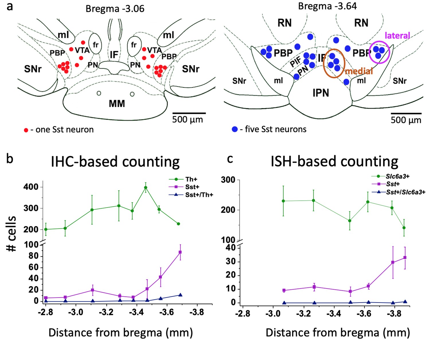
Localization and number of Sst and DA neurons in the mouse VTA.
(a) Schematic representation of lateral and medial Sst neuron clusters in coronal sections at different distances from bregma: the left figure represents the rostral VTA with only lateral clusters and small number of cells (each red dot = one Sst neuron); the right figure of the caudal VTA shows medial (PIF+PN) and lateral (PBP) cell clusters and a higher number of cells (each blue dot = 5 Sst cells). IF, interfascicular nucleus; IPN, interpeduncular nucleus; MM, medial mamillary nucleus; PBP, parabrachial pigmented nucleus; PIF, parainterfascicular nucleus; PN, paranigral nucleus; RN, red nucleus; SNr, substantia pars reticulata; VTA, ventral tegmental area (rostral part); ml, medial lemniscus; fr, fasciculus retroflexus. (b) Cell counts for DA and Sst cells using immunohistochemical (IHC) approach: Th-antibody staining for DA neurons combined with inbuilt dTomato signal for Sst neurons of Sst-tdTomato mice. Number of cells is given per 40-µm-thick coronal section as mean ± SEM (n = 3 mice) at different levels from bregma along the rostro-caudal axis. (c) Cell counts, using in situ hybridization (ISH) approach with RNAscope probes for Sst and Slc6a3 mRNAs. Number of cells is given per 12-µm-thick coronal section as mean ± SEM (n = 4 mice). The number of Sst neurons (magenta) increased in more caudal part of the VTA with both staining methods. Supporting data can be found in the Additional files: Figure 1—source data 1. Figure 1—figure supplement 1.
-
Figure 1—source data 1
Raw data for Figure 1b–c.
- https://cdn.elifesciences.org/articles/59328/elife-59328-fig1-data1-v2.xlsx
Figure 1—figure supplement 1
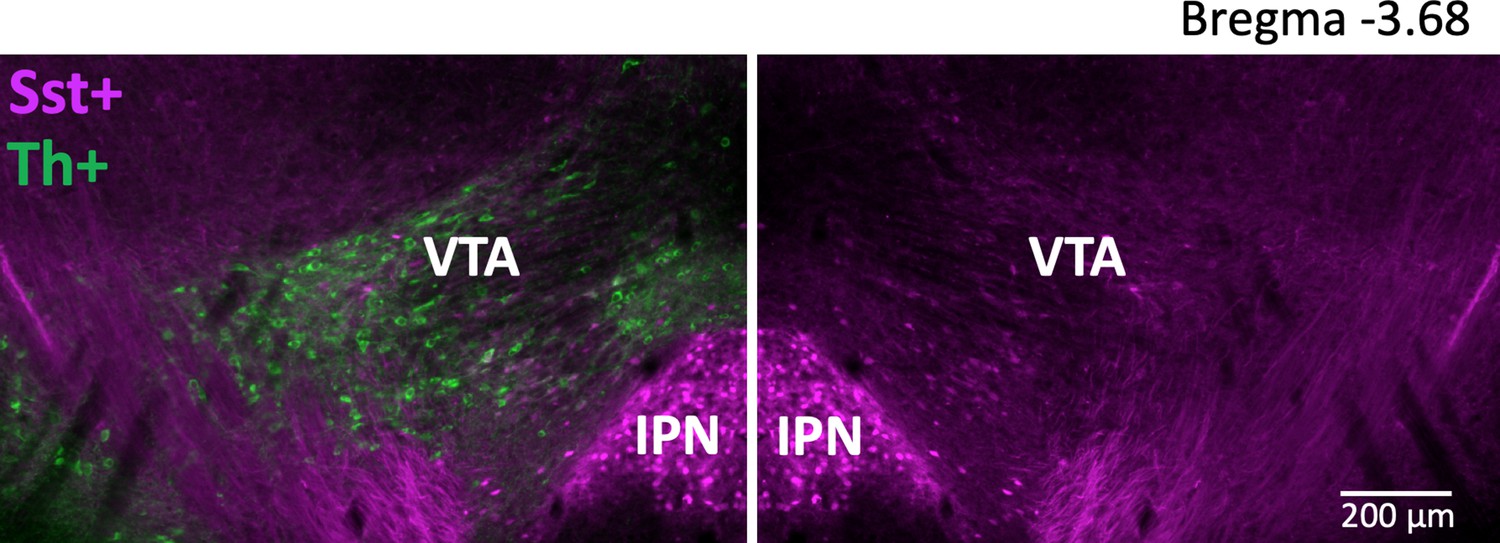
Anatomical localization of Sst neurons within the VTA in coronal plane.
A representative image of coronal sections, which were used for IHC-based counting. The VTA was defined by Th+ staining (excluding the substantia nigra compacta) – left image. Right image shows the magenta Sst cells in the same section (horizontally flipped) with the green Th+ channel off.
Figure 2
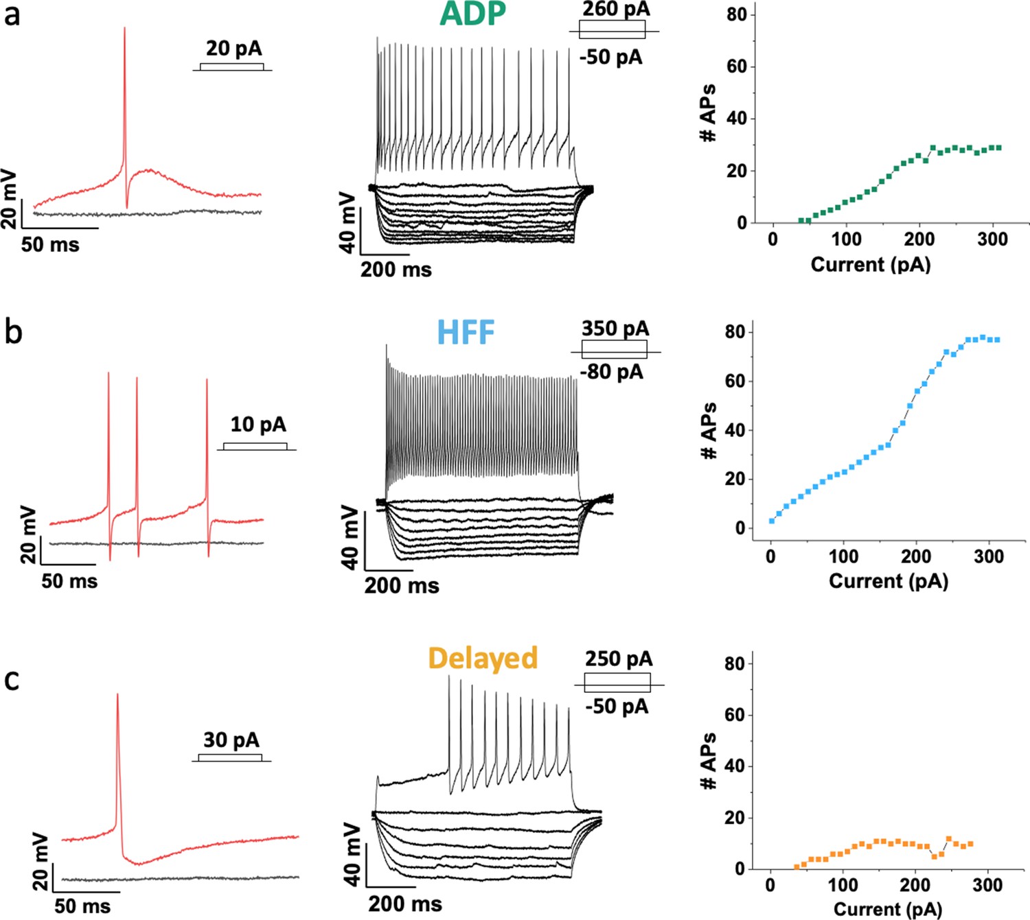
Three major Sst-expressing neuron subtypes in the VTA based on their firing properties.
From left to right: example traces of the action potentials (APs) (in red) evoked by rheobase current injection, black line represents the baseline with no current injected; example traces of subthreshold voltage-responses of the same cells to 800 ms current steps with 10 pA increment, together with voltage-responses to saturated excitation; cumulative spike counts after increasing currents steps. (a) ADP neurons showed salient afterdepolarization (ADP) at rheobase current and a visible adaptation in firing at the saturated level of excitation. (b) High-frequency firing neurons (HFF) displayed sharp prominent afterhyperpolarization at rheobase current and the highest number of APs at the saturated level of excitation. (c) Delayed neurons demonstrated a long delay preceding the firing at the saturated level of excitation. Slow afterhyperpolarization and low adaptation were distinctive features of this particular subtype.
Figure 3 with 4 supplements
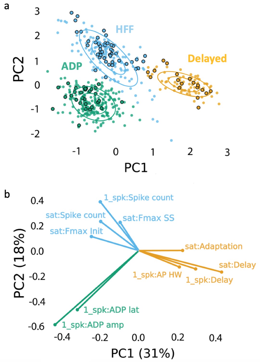
Clustering approach for electrophysiological subtyping of the Sst-expressing neurons.
Afterdepolarizing ‘ADP’ subtype is in green, high-frequency firing ‘HFF’ subtype in light blue, and ‘Delayed’ subtype in yellow. (a) Scatter plot of the Sst-neuron subtypes depicting the results of PCA (PC1 and PC2 as ‘x’ and ‘y’ axes, respectively) and GMM (big circles in corresponding colors). Non-outlined dots denote the cells from juvenile mice (n = 392), while black-outlined dots represent mature neurons from P60-P90 mice (n = 92): mature neurons reproduced the clustering pattern of younger neurons. (b) PCA weights of the electrophysiological characteristics that most influenced the clustering (see also Table 1). Clustering script and intermediate electrophysiological data to reproduce the results can be downloaded from here: https://version.aalto.fi/gitlab/zubarei1/clustering-for-nagaeva-et.-al.-sst-vta. Supporting data can be found in the Additional files: Figure 3—figure supplements 1–4.
Figure 3—figure supplement 1
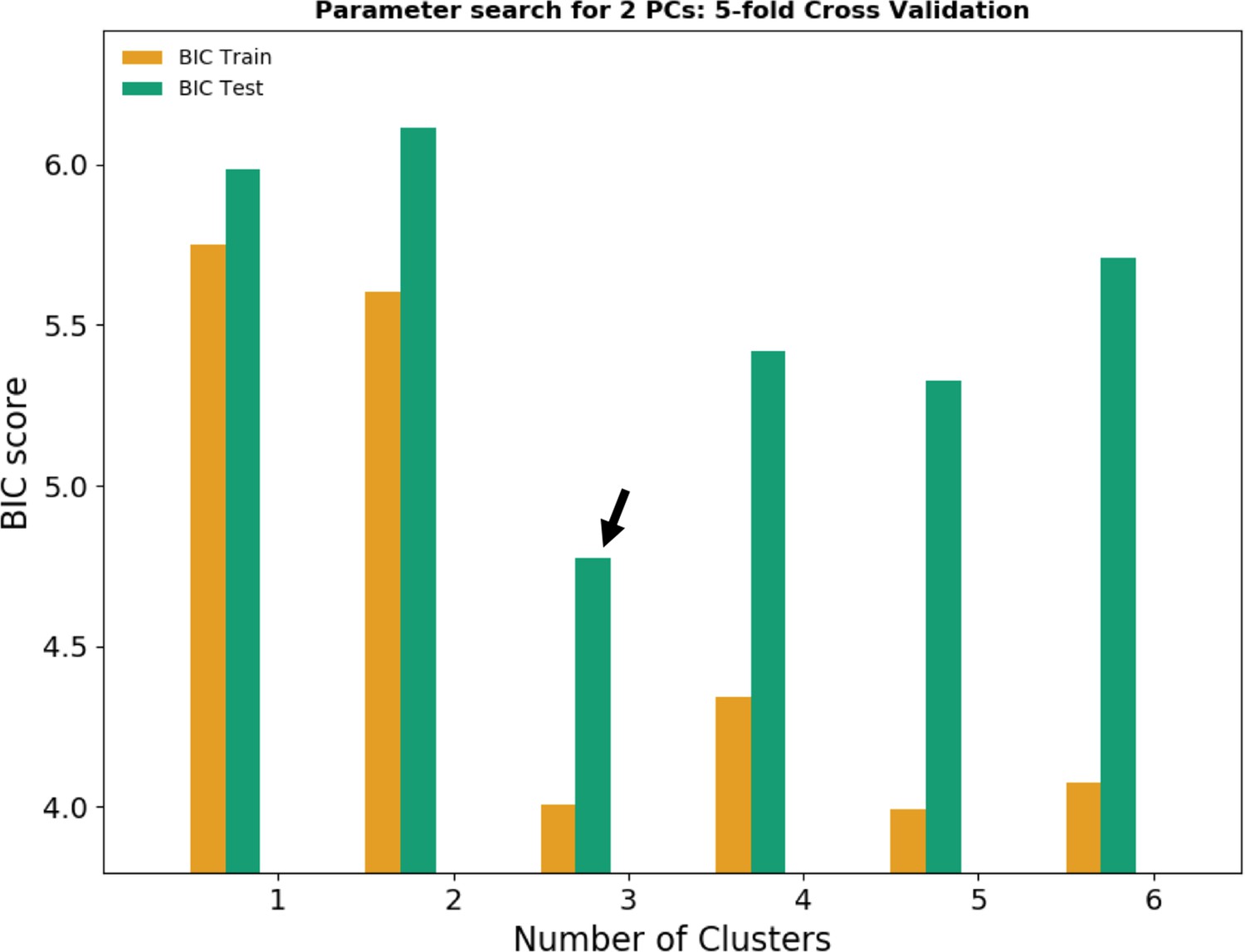
Bayesian information criterion (BIC) for model selection.
According to the BIC, the combination of two principal components (PCs) and three clusters gives the best fit to describe the data (black arrow). Orange bars represent the BIC score for the model training dataset; green bars represent the BIC score for the test dataset unfamiliar to the model.
Figure 3—figure supplement 2
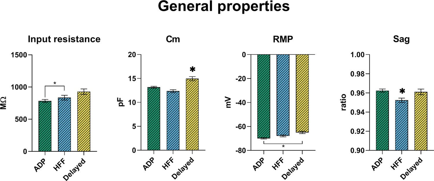
Passive membrane properties of VTA Sst-neuron subtypes.
Cm, cell capacitance; RMP, resting membrane potential. All graphs show means ± SEM for ADP (n = 215), HFF (n = 92) and Delayed (n = 85) neurons. Statistical significances between groups were measured by one-way ANOVA with Tukey’s post hoc test. Big asterisks show values, which are significantly different from two others (p<0.05). Small asterisks with the connecting line indicate only two significantly different values.
Figure 3—figure supplement 3
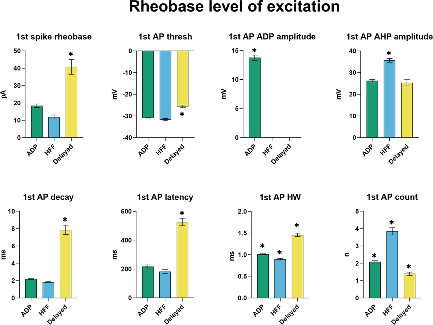
Electrophysiological properties of the first action potential (AP) at rheobase level of excitation.
ADP, afterdepolarization; AHP; afterhyperpolarization; HW, half-width. All graphs show means ± SEM for ADP (n = 215), HFF (n = 92) and Delayed (n = 85) neurons. Statistical significances between groups were measured by one-way ANOVA with Tukey’s post hoc test. Big asterisks show values, which are significantly different from two others (p<0.05). Small asterisks with the connecting line indicate only two significantly different values.
Figure 3—figure supplement 4
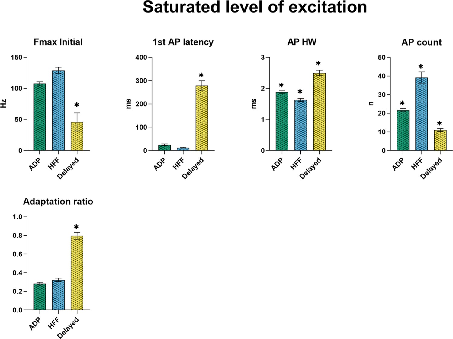
Electrophysiological properties of the subtypes at the saturating level of excitation, producing the highest number of action potentials.
All graphs show means ± SEM for ADP (n = 215), HFF (n = 92) and Delayed (n = 85) neurons. Statistical significances between groups were measured by one-way ANOVA with Tukey’s post hoc test. Big asterisks show values, which are significantly different from two others (p<0.05). Small asterisks with the connecting line indicate only two significantly different values.
Figure 4
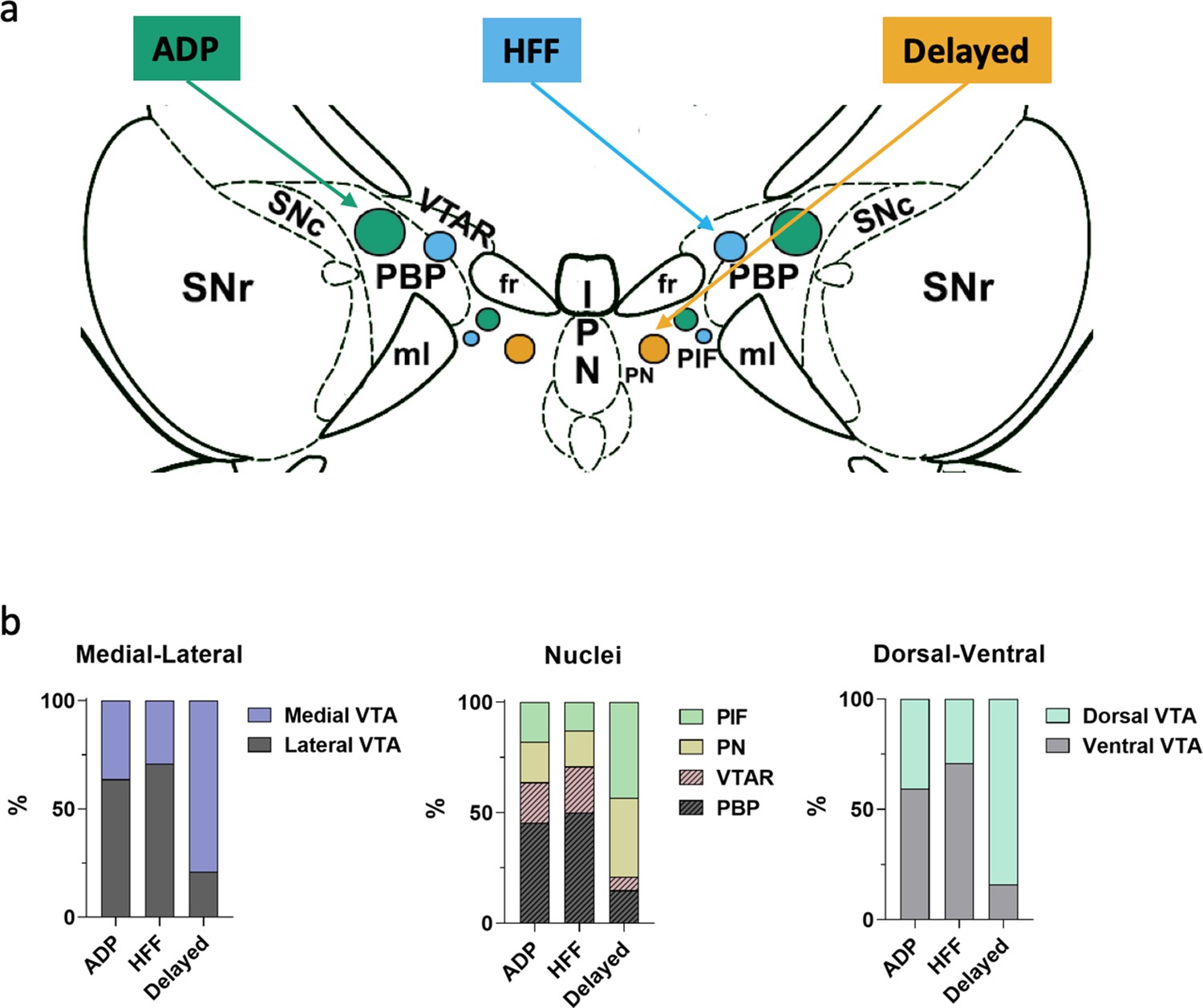
Differential localizations of Sst-expressing neuron subtypes within the VTA.
(a) Schematic depiction of subtype locations within the VTA horizontal slice (bregma −4.44 mm). Circle sizes represent relative number of cells. SNc, substantia nigra pars compacta; VTAR, ventral tegmental area, rostral part; the other abbreviations as defined in Figure 1a. (b) Lateral part of the VTA is represented by PBP and VTA nuclei, and the medial part by PIF and PN nuclei, in accordance with the Mouse Brain Atlas (Franklin and Paxinos, 2008). The ventral VTA was defined from −4.72 to −4.56 mm, and the dorsal VTA from −4.44 to −4.28 mm in horizontal plane. The Delayed neurons were preferentially localized in the mediodorsal VTA, while the ADP and HFF neurons lateroventrally.
Figure 5 with 2 supplements

Morphological properties of the Sst-expressing neuron subtypes.
(a) Significantly different morphological characteristics between the three electrophysiological subtypes. Mean intersections, a parameter from Sholl analysis, shows how many times a circle of one radius intersects neuronal processes. All graphs show means ± SEM for ADP neurons (n = 21), HFF neurons (n = 8) and Delayed neurons (n = 20). Asterisks indicate values statistically different from two others (cell body area: F(2, 46)=5.565, p=0.0068; # processes: F(2, 46)=9.745, p=0.0003; # branching points: F(2, 46)=6.974, p=0.0023; mean intersections: F(2, 46)=5.280, p=0.0086). (b) Example of a Delayed neuron morphology with color-coded circles, produced by Sholl analysis: from red to blue for minimum to maximum number of intersections, respectively. White line crossing the cell body corresponds to the direction of the sagittal plane and ‘midline’ indicates center of the slice close to the interpeduncular nuclei (IPN, see also Figure 4a). (c) Average Sholl curves for the electrophysiological subtypes, showing that Delayed neurons had the largest number of intersections within 100 µm from the cell body. Morphology of the traced neurons and individual Sholl curves can be found in Additional files: Figure 5—source datas 1–2. Figure 5—figure supplements 1–2.
-
Figure 5—source data 1
raw data for Figure 5a.
- https://cdn.elifesciences.org/articles/59328/elife-59328-fig5-data1-v2.xlsx
-
Figure 5—source data 2
File Morphology_Source.zip: source files for morphology and location.
This zip archive contains morphological images of all traced neurons grouped according their electrophysiological profiles. Each subtype’s folder contains a PDF file (with the list of neurons, their original location within the VTA, images of the traced morphology and individual Sholl curves) and two subfolders: ‘3D_gif’ – with *.gif files of the listed neurons; and ‘WaveFront_3D_obj’ – with corresponding *.obj files. *.gif files can be opened by any image viewer. *.obj files save information about the 3D model of the neurons and can be opened/reused with any 3D viewer or graphic software.
- https://cdn.elifesciences.org/articles/59328/elife-59328-fig5-data2-v2.zip
Figure 5—figure supplement 1

Examples of VTA Sst-neuron morphology.
From the left, line by line: black and white-inverted copies of original micrographs of neurobiotin-filled Sst cells of the ADP, HFF and Delayed subtypes defined by clustering according to their electrophysiological features. Middle: reconstructed morphology of the same neurons. Right: the Sholl curves for the same cells.
Figure 5—figure supplement 2
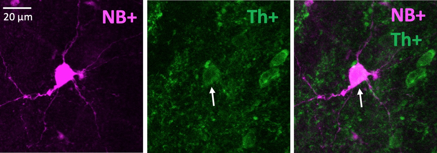
An example of a neurobiotin-filled (NB+) Delayed neuron with positive Th staining.
Figure 6 with 4 supplements
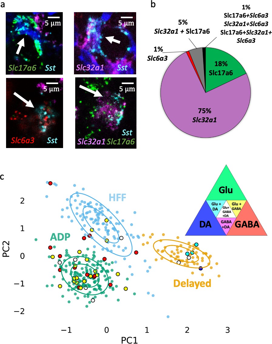
Neurochemical phenotypes of VTA Sst neurons according in situ mRNA hybridization and PatchSeq experiments.
(a) Example images of multichannel in situ hybridization RNAscope experiments, showing a variety of Sst neuron molecular subtypes, based on Sst, Slc6a3, Slc32a1 and Slc17a6 mRNA expressions. (b) Proportion of Sst neuron molecular subtypes, as classified and counted for coronal and horizontal sections of the VTA from adult wild-type C57BL/6J mice (n = 8). (c) Molecular subtypes, acquired by alignment of PatchSeq results to a bigger midbrain scRNASeq database, mapped on electrophysiological Sst-neuron clusters (see Figure 3a). Triangle in the right corner shows color-coding for the molecular subtypes. ADP and HFF clusters included mostly GABA or Glu+GABA neurons, whereas the Delayed cluster had a spectrum of DA-containing neurons. Supporting data can be found in the Additional files: Figure 6—source data 1. Figure 6—figure supplements 1–4.
-
Figure 6—source data 1
Raw data for Figure 6b–c.
- https://cdn.elifesciences.org/articles/59328/elife-59328-fig6-data1-v2.xlsx
Figure 6—figure supplement 1
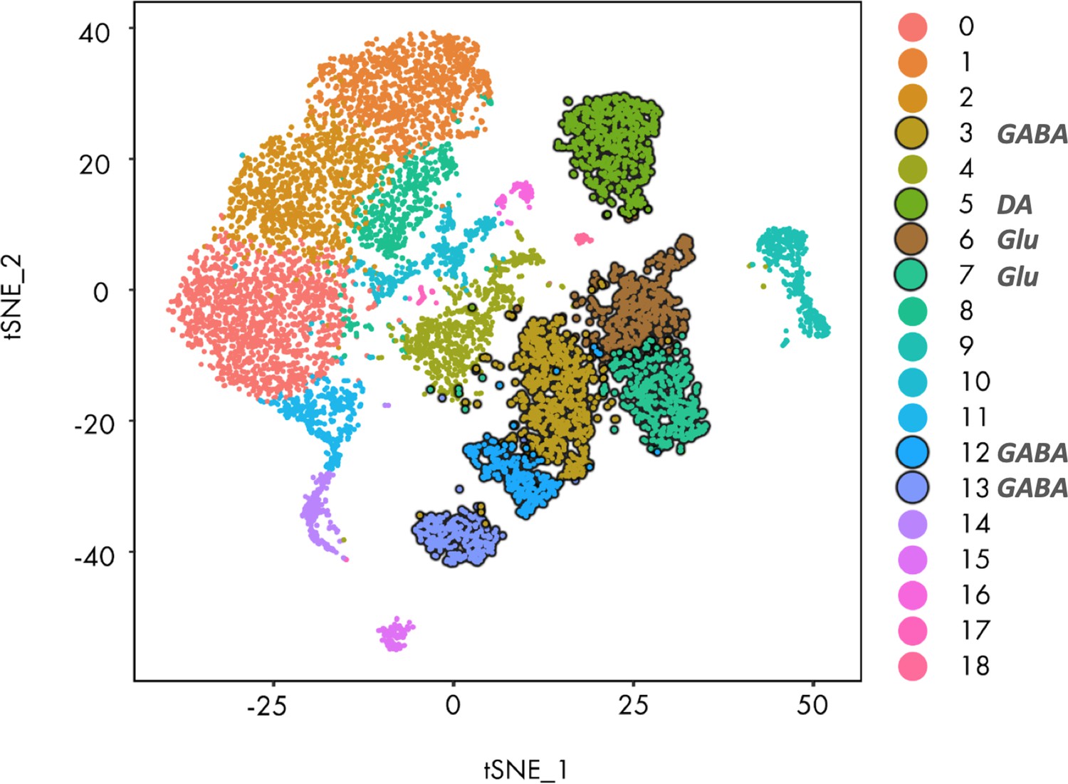
Seurat clustering of the reference midbrain dataset and selection of the clusters for PatchSeq cells classification.
tSNE of the clustering results. Clusters highlighted with dark contours were used for the mapping procedure. Clusters 3, 5, 6, 7, 12 and 13 were selected due to Sst (panel b) and neuronal markers expression (panel c).
Figure 6—figure supplement 2

Sst expression in selected clusters 3, 5, 6, 7, 12 and 13.
Figure 6—figure supplement 3
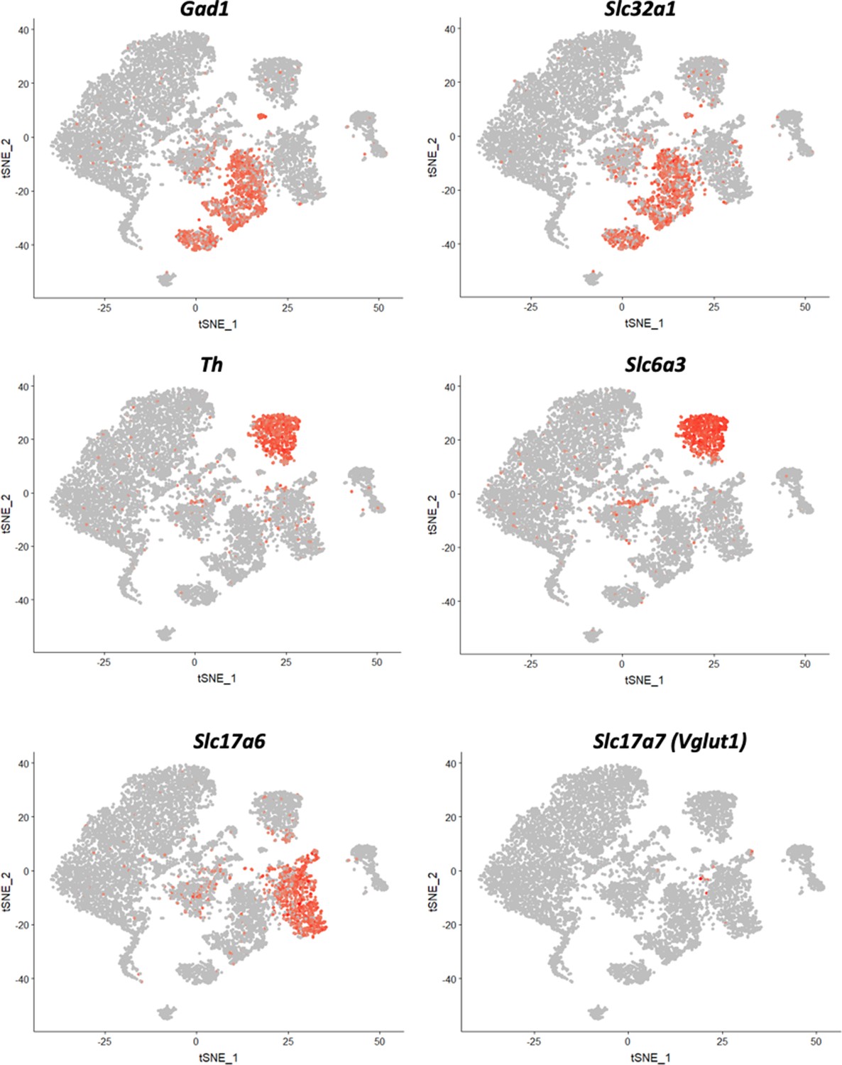
Neuronal marker expression in selected clusters 3, 5, 6, 7, 12 and 13.
Figure 6—figure supplement 4

Expression of dopamine-related genes in different Sst-expressing neuronal populations in the VTA, indicating strong expression in Delayed cells.
Values are mean expression levels in read counts for n cells. For scaling, the values for Th were divided by 10.
Figure 7 with 2 supplements
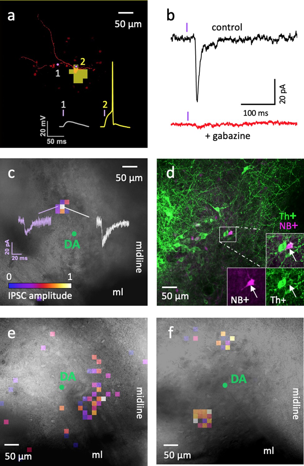
Optogenetic circuit mapping: a single VTA DA neuron can be inhibited by more than one ADP Sst-expressing neuron.
(a) Representative example of the optical footprint of a Sst neuron stimulated with 405 nm laser spots of 9 µW power. The neuron was filled with Alexa 594 dye through patch pipette. Optical footprint, illustrating the square spots where laser stimulation induced action potential in the ADP subtype of Sst cells, is shown in yellow pixels and located around the cell body. Traces 1 and 2 demonstrate evoked responses, while stimulating the corresponding point around the Sst cell. Action potential (2) was induced by stimulation on the soma, while no action potentials were induced by laser spots on the neurites (1). (b) The black trace (‘control’) shows an IPSC evoked in DA cell due to optical stimulation of a neighboring ADP neuron. The red trace shows an absence of evoked IPSCs in the same cell during application of the GABAA receptor antagonist gabazine (10 µM). The violet bars indicate moments of the light (405 nm) flash. (c) Colored pixels represent input maps from a Sst neuron to a neighboring DA cell (shown as a green circle in the center) at 9 μW laser power setting. Amplitudes of the optically evoked IPSCs were color-coded according to the pseudocolor scale, shown at the bottom in relative units from 0 to 1 (used also in panels e and f). Actual amplitudes varied between experiments and are here shown in white (corresponds to maximum IPSC amplitude of 40 pA) and purple (corresponds to IPSC amplitude of 20 pA) traces. (d) Post-staining of the neurobiotin-filled postsynaptic DA neuron shown in c; the cell is labeled with streptavidin 633 (magenta, NB+) and tyrosine hydroxylase antibody (green, Th+). (e–f) Two other examples of input maps at 9 µW demonstrate their variability. All circuit maps in c, e and f overlay images of horizontal VTA slices, where recordings were carried out showing location of the DA cells. Maps in c and e were recorded at bregma −4.44 and that in f at bregma −4.56. ml, medial lemniscus; ‘midline’ indicates the sagittal center line of the horizontal slice. Supporting data can be found in the Additional files: Figure 7—figure supplements 1–2.
Figure 7—figure supplement 1

Examples of Ih-current test (a) and immunohistochemistry (b) for confirmation of DA neuron phenotype.
(a) Ih current is shown as an extra inward current, occurring during hyperpolarization of the cell membrane potential from −70 to −130 mV. (b) The recorded DA neuron was positive for Neurobiotin (magenta) and Th (green). Often Th was leaking out from the cell body during neurobiotin loading, explaining why many cells are brighter co-stained at axonic/dendritic sites than at somas.
Figure 7—figure supplement 2
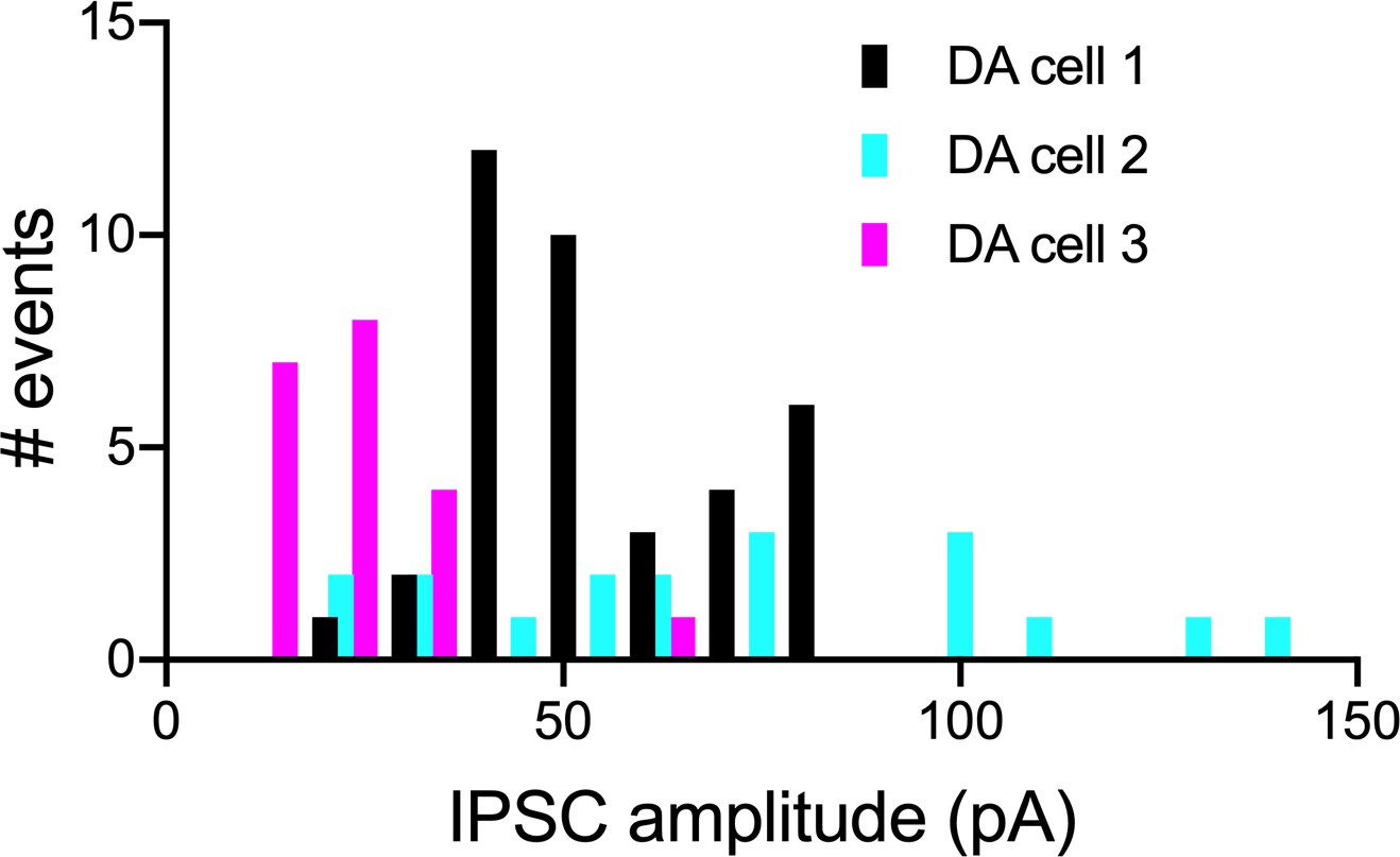
Examples of amplitude variations of evoked IPSCs in VTA DA cells.
ADP-subtype Sst neurons were activated by repeated laser spots at 9 mW power, which resulted in IPSCs in local DA cells. IPSC frequencies are shown by number of events, one event being a mean of three IPSCs evoked by the stimulation of the same anatomical spot. Events for three representative DA cells are shown to illustrate the variation in amplitudes between and within the cells. Supporting data can be found in the Additional files: Figure 7—figure supplement 2—source data 1.
-
Figure 7—figure supplement 2—source data 1
Raw data for Figure 7—figure supplement 2.
- https://cdn.elifesciences.org/articles/59328/elife-59328-fig7-figsupp2-data1-v2.xlsx
Figure 8
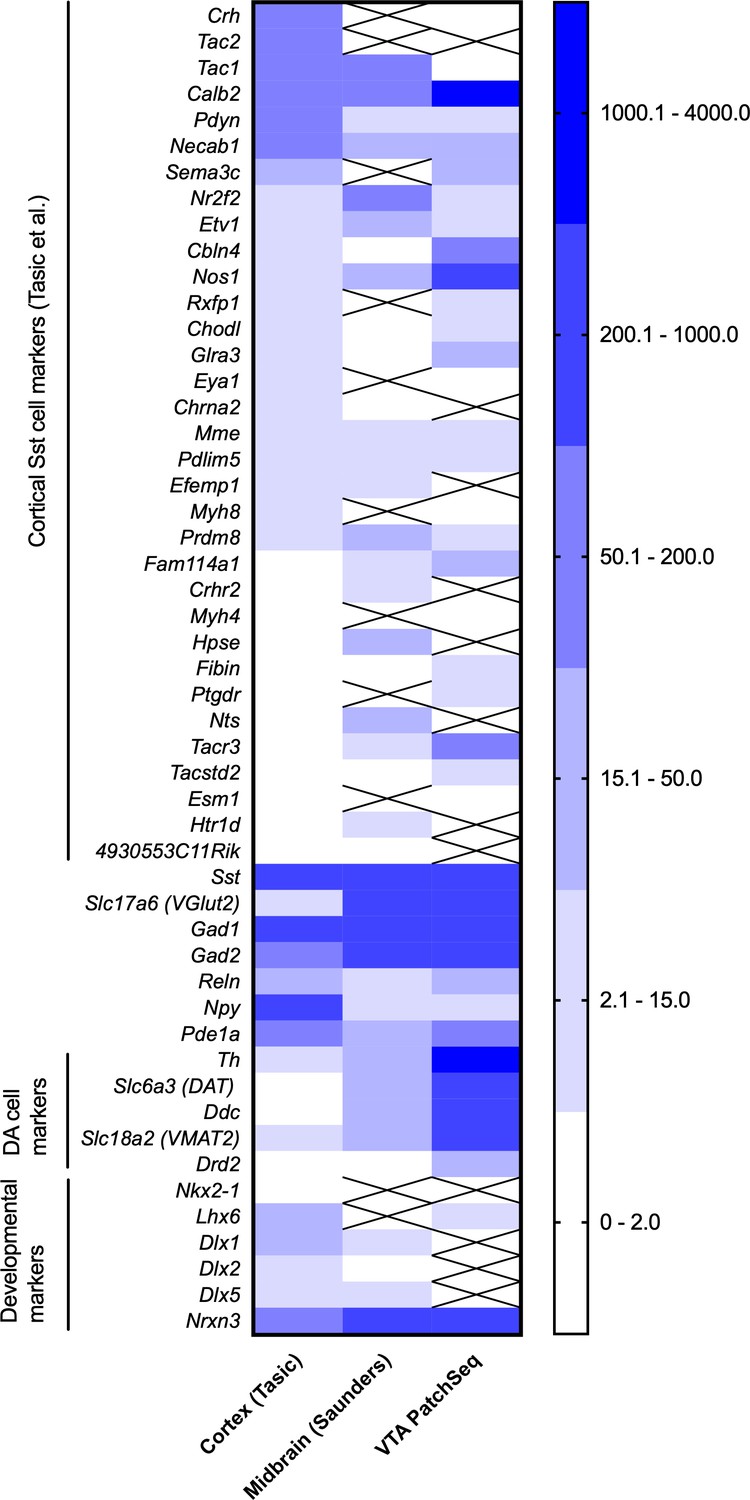
Comparison of expression of genes of interest in neocortical Sst neurons (Tasic et al., 2018), Sst neurons of the midbrain (Saunders et al., 2018) and in the PatchSeq cells of the present study.
The three sets were normalized by setting the Sst expression to 1000. Crossed out means ‘no expression’ in the dataset.
Videos
Video 1
https://vimeo.com/422563851 A video abstract illustrates three subtypes of somatostatin neurons, described in the article, with their original morphology (traced with neurobiotin with further 3D reconstruction), firing patterns (recorded with patch-clamp method).
It also shows location of these neurons within ventral tegmental area (VTA), midbrain and the whole mouse brain. Video has been made by a media artist Nikolai Larin. 3D Mouse brain credit: Allen Institute.
Tables
Table 1
Electrophysiological properties of the three Sst neuron subtypes in the VTA.
| General | ADP (n = 215) | HFF (n = 92) | Delayed (n = 85) |
|---|---|---|---|
| Input resistance (MΩ) | 783 ± 24 | 835 ± 37 | 928 ± 42 |
| RMP (mV) | −69.9 ± 0.6 | −67.8 ± 0.8 | −64.9 ± 1.0 |
| Cm (pF) | 13.2 ± 0.2 | 12.4 ± 0.3 | 15.0 ± 0.4* |
| Sag | 0.963 ± 0.002 | 0.952 ± 0.002* | 0.961 ± 0.003 |
| 1 st spike at rheobase current | |||
| Rheobase current (pA) | 18.4 ± 1.0 | 11.9 ± 1.2 | 40.8 ± 4.3* |
| AP threshold (mV) | −31.1 ± 0.3 | −31.7 ± 0.5 | −25.6 ± 0.6 |
| AP amplitude (mV) | 95.2 ± 0.6 | 94.0 ± 0.8 | 87.9 ± 0.8* |
| ADP amplitude (mV) | 13.8 ± 0.5* | no ADP | no ADP |
| 1 st AP delay (ms) | 218 ± 10 | 182 ± 14 | 528 ± 25* |
| AP half-width (ms) | 1.01 ± 0.01* | 0.90 ± 0.02* | 1.46 ± 0.04* |
| AHP amplitude (mV) | 26.3 ± 0.5 | 35.7 ± 0.9* | 25.3 ± 1.5 |
| AP decay (ms) | 2.2 ± 0.1 | 1.84 ± 0.04 | 7.9 ± 0.5* |
| Spike count | 2.1 ± 0.1* | 3.9 ± 0.2* | 1.4 ± 0.1* |
| Saturated level of excitation | |||
| Saturating current step (pA) | 207 ± 5 | 209 ± 11 | 242 ± 12 |
| Fmax initial (Hz) | 108 ± 3 | 129 ± 5 | 46 ± 15* |
| Fmax steady state (Hz) | 25.6 ± 1.1 | 42.9 ± 3.7 | 21.2 ± 1.4 |
| Adaptation ratio | 0.28 ± 0.02 | 0.32 ± 0.02 | 0.80 ± 0.04* |
| 1 st AP delay (ms) | 24.8 ± 3.4 | 12.2 ± 1.2 | 279.0 ± 20.4* |
| AP half-width (ms) | 1.88 ± 0.04* | 1.6 ± 0.1* | 2.5 ± 0.1* |
| Spike count | 21.6 ± 0.9* | 39.1 ± 3.1* | 11.00 ± 0.8* |
-
Data are shown as means ± SEM. Asterisks indicate values statistically different from two others (p<0.05). Row colors indicate important features, which influenced unsupervised clustering (Figure 3a–b).
Key resources table
| Reagent type (species) or resource | Designation | Source or reference | Identifiers | Additional information |
|---|---|---|---|---|
| Genetic reagent (M. musculus) | Ssttm2.1(cre)Zjh//J; Sst-IRES-Cre | The Jackson Laboratory | RRID:IMSR_JAX:013044 | |
| Genetic reagent (M. musculus) | B6.Cg-Gt(ROSA)26Sortm14(CAG-tdTomato)Hze/J; Ai14 | The Jackson Laboratory | RRID:IMSR_JAX:007914 | |
| Genetic reagent (M. musculus) | B6;129S-Gt(ROSA)26Sortm32(CAG-COP4*H134R/EYFP)Hze/J | The Jackson Laboratory | RRID:IMSR_JAX:012569 | |
| Strain, strain background (M. musculus) | C57BL/6J | The Jackson Laboratory | 000664; RRID:IMSR_JAX:000664 | |
| Antibody | Anti-tyrosine hydroxylase (Rabbit polyclonal) | Sigma-Aldrich | Cat# AB152, RRID:AB_390204 | IHC: 1:100 |
| Antibody | Anti-rabbit IgG H and L Alexa Fluor 488 (Goat polyclonal) | Invitrogen | Cat# A-11008, RRID:AB_143165 | IHC: 1:1000 |
| Peptide, recombinant protein | Streptavidin, Alexa Fluor 633 conjugate | Thermo Fisher | Cat# S-21375, RRID:AB_2313500 | (1:1000) |
| Software, algorithm | Zeiss ZEN 2 (Blue) | Zeiss | RRID:SCR_013672 | |
| Software, algorithm | Leica Application Suite X | Leica | RRID:SCR_013673 | |
| Software, algorithm | Fiji Image J | Fiji https://imagej.net/Fiji/Downloads | RRID:SCR_003070; | Version 1.51; Plugins: Neurite Tracer |
| Software, algorithm | MATLAB | Mathworks (https://www.mathworks.com/) | RRID:SCR_001622 | Version R2018b; custom script for electrophysiological analysis https://github.com/zubara/fffpa |
| Software, algorithm | pClamp | Molecular devices | RRID:SCR_011323 | Clampex 8.2 and 10, Clampfit 10.7 |
| Software, algorithm | R Project for Statistical Computing | https://www.r-project.org | RRID:SCR_001905 | Version 3.5; Seurat 2.3.4 https://satijalab.org/seurat/install.html and EWCE (https://github.com/NathanSkene/EWCE) packages for scRNAseq analysis |
| Software, algorithm | Python Programming Language | https://www.python.org | RRID:SCR_008394 | Version 3.6; custom script for electrophysiological clustering analysis https://version.aalto.fi/gitlab/zubarei1/clustering-for-nagaeva-et.-al.-sst-vta |
| Software, algorithm | CSC Chipster | CSC – IT center for science LTD. (csc.fi) | https://chipster.csc.fi | HISAT2 and HTSeq implementations |
| Software, algorithm | Graphpad Prism | Graphpad | RRID:SCR_002798 | Version 8.1 |
| Commercial assay or kit | RNAScope probe Mm-Slc6a3 | Advanced Cell Diagnostics | ACD: 315441 | |
| Commercial assay or kit | RNAScope probe Mm-Slc17a6 | Advanced Cell Diagnostics | ACD: 319171-C2 | |
| Commercial assay or kit | RNAScope probe Mm-Sst | Advanced Cell Diagnostics | ACD: 404638 | |
| Commercial assay or kit | RNAScope probe Mm-Slc32a1 | Advanced Cell Diagnostics | ACD: 319191 |
Additional files
Download links
A two-part list of links to download the article, or parts of the article, in various formats.
Downloads (link to download the article as PDF)
Open citations (links to open the citations from this article in various online reference manager services)
Cite this article (links to download the citations from this article in formats compatible with various reference manager tools)
Heterogeneous somatostatin-expressing neuron population in mouse ventral tegmental area
eLife 9:e59328.
https://doi.org/10.7554/eLife.59328


