A single-cell atlas of the mouse and human prostate reveals heterogeneity and conservation of epithelial progenitors
- Department of Medicine, Columbia University Irving Medical Center, United States
- Department of Genetics and Development, Columbia University Irving Medical Center, United States
- Department of Urology, Columbia University Irving Medical Center, United States
- Department of Systems Biology, Columbia University Irving Medical Center, United States
- Herbert Irving Comprehensive Cancer Center, Columbia University Irving Medical Center, United States
- Department of Biomedical Informatics, Columbia University Irving Medical Center, United States
- Department of Pathology and Laboratory Medicine, Weill Medical College of Cornell University, United States
- Department of Pathology and Cell Biology, Columbia University Irving Medical Center, United States
Figures
Figure 1 with 5 supplements
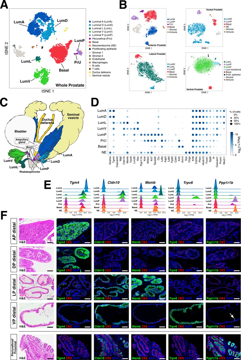
Single-cell analysis identifies prostate luminal epithelial heterogeneity.
(A) t-distributed stochastic neighbor embedding (tSNE) plot of 5288 cells from an aggregated dataset of two normal mouse prostates, processed by Randomly and clustered using the Leiden algorithm. (B) tSNE representation of each prostate lobe (AP: 2735 cells; DP: 1781 cells; LP: 2044 cells; VP: 1581 cells). (C) Schematic model of prostate lobes with the urethral rhabdosphincter partially removed, with the distribution of luminal epithelial populations indicated. (D) Dot plot of gene expression levels in each epithelial population for selected marker genes. (E) Ridge plots of marker genes showing expression in each population. (F) Hematoxylin-eosin (H and E) and immunofluorescence (IF) images of selected markers in serial sections; the periurethral/proximal region shown is from the AP and DP. Arrow in VP distal indicates distal cell with Ppp1r1b expression. Scale bars indicate 50 µm.
Figure 1—figure supplement 1
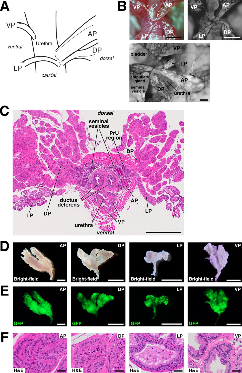
Anatomy and dissection of mouse prostate lobes.
(A) Schematic of connections of prostate lobes to the urethra. Note that the AP, DP, and LP connect dorsally in close proximity, whereas the VP connects on the ventral side. (B) Whole-mount views of prostate lobe connections in UBC-GFP mice. (C) H and E staining of transverse section through intact urogenital apparatus. The LP crosses the rhabdosphincter caudally (right), and the periurethral (PrU) region lies within the rhabdosphincter. (D,E) Bright-field and epifluorescence views of dissected prostate lobes from UBC-GFP mouse. Proximal regions are oriented downwards; note that the LP is the smallest lobe and has a relatively long unbranched region. (F) H and E staining of sections from the indicated lobes. Scale bars in (B–E) indicate 2 mm, in (F) indicate 50 µm.
Figure 1—figure supplement 2

Random-matrix analysis of single-cell datasets.
Comparison of dimensional reduction, clustering and visualization of 2322 sequenced cells from the mouse anterior lobe, based on traditional PCA (A–D), and the Randomly algorithm (E–J). (A) 'Elbow plot' describing the variance ratio of each principal component (PC) after a PCA reduction of the log2(1+TPM) transformed count matrix. (B) Mean silhouette scores of the clusters obtained for different values of the Leiden resolution after performing a clustering in the first 11 PCs using the Leiden algorithm (as implemented in Wolf et al., 2018). (C,D) tSNE visualizations of the 11 PCs and clustering for Leiden resolutions of 0.2 (7 clusters) and 0.3 (8 clusters), respectively. The LumA* cells have similar expression profiles as the LumA population, but display altered expression of ribosomal and mitochondrial genes, which is consistent with cellular stress. (E) Normality test to detect eigenvector localization in the 2322 cell-eigenvectors of the z-scored log2(1+TPM) transformed count matrix. The red line corresponds to the sparse data before Randomly and the green line shows eigenvector behavior after elimination of the sparsity-induced signal. (F) Spectral distribution of the Wishart matrix for selected cells after elimination of the sparsity-induced signal (blue histogram) with a Marchenko-Pastur (MP) distribution fit (red line). Only 50 eigenvalues (~2% of the total) lie outside the MP distribution, and their corresponding eigenvectors carry true signal. The remaining ~98% of the data is comparable to a random matrix and is therefore noise. (G) Chi-squared test for the variance of the genes’ projection into different sets of eigenvectors. Blue, the 50 signal-like eigenvectors; pink, the eigenvectors corresponding to the last 50 MP eigenvalues; green, the eigenvectors corresponding to the first 50 MP eigenvalues; brown, projection on 50 2,322-dimensional random vectors. (H) Selection of the genes that are mostly responsible for the signal in this dataset (purple line). The number of genes (orange line) is calculated with a false discovery rate (FDR) using the ratio of the blue and pink distributions in (G) Approximately 5000 genes are responsible for the signal using FDR . (I) Mean silhouette score of the clusters obtained for different values of the Leiden resolution after processing with Randomly. In comparison with (B), the score is much higher, indicating better clustering. (J) tSNE visualization of the latent space generated by Randomly and clustering performed with the Leiden algorithm. For downstream analyses, we have combined the LumA* cells with the LumA population. The number of clusters selected corresponds to the maximum of the curve in (I). Randomly can assist in identification of populations (e.g. PrU) by removing noise and sparsity-induced signals, and by selecting genes responsible for the biological signal.
Figure 1—figure supplement 3
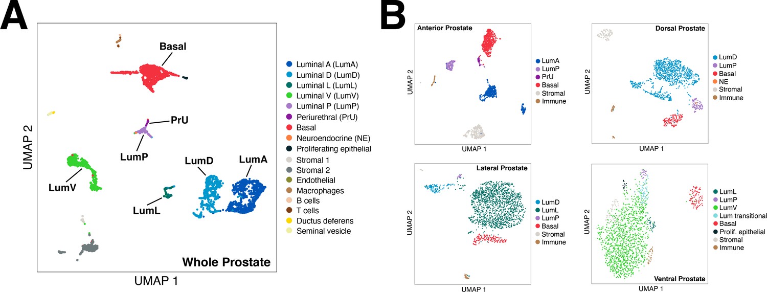
UMAP plots of mouse single-cell RNA-seq data.
Figure 1—figure supplement 4
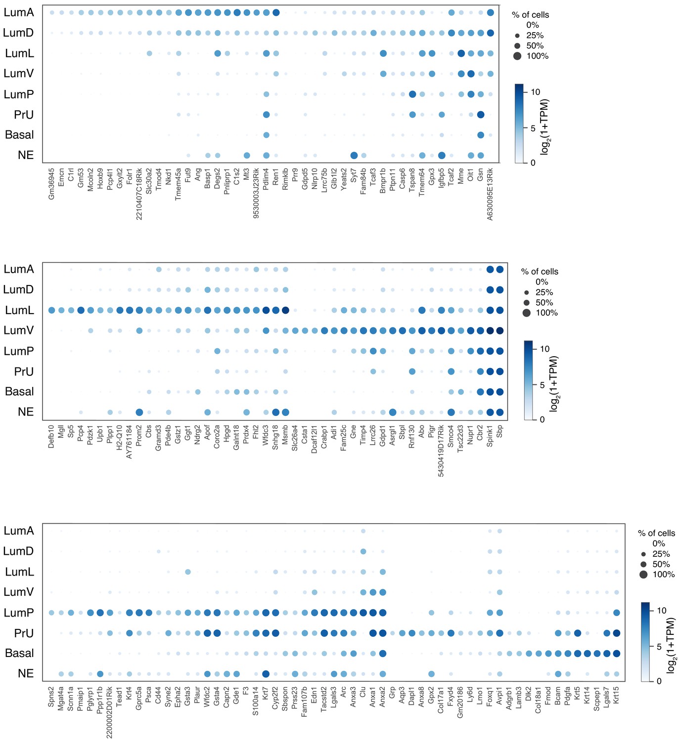
Dot plot of expression levels for selected genes in each epithelial population.
An expanded list of genes is shown to complement the dot plot in Figure 1D.
Figure 1—figure supplement 5
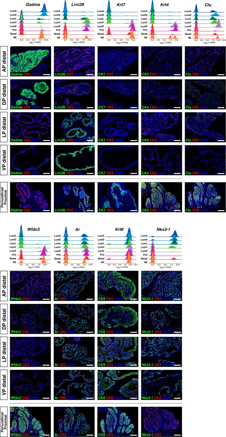
Additional marker validation for epithelial populations.
(Above) Ridge plots of marker genes show expression in each population. (Below) Immunofluorescence staining of marker expression in sections; the periurethral/proximal region shown is from the AP and DP. Scale bars indicate 50 µm.
Figure 2 with 1 supplement
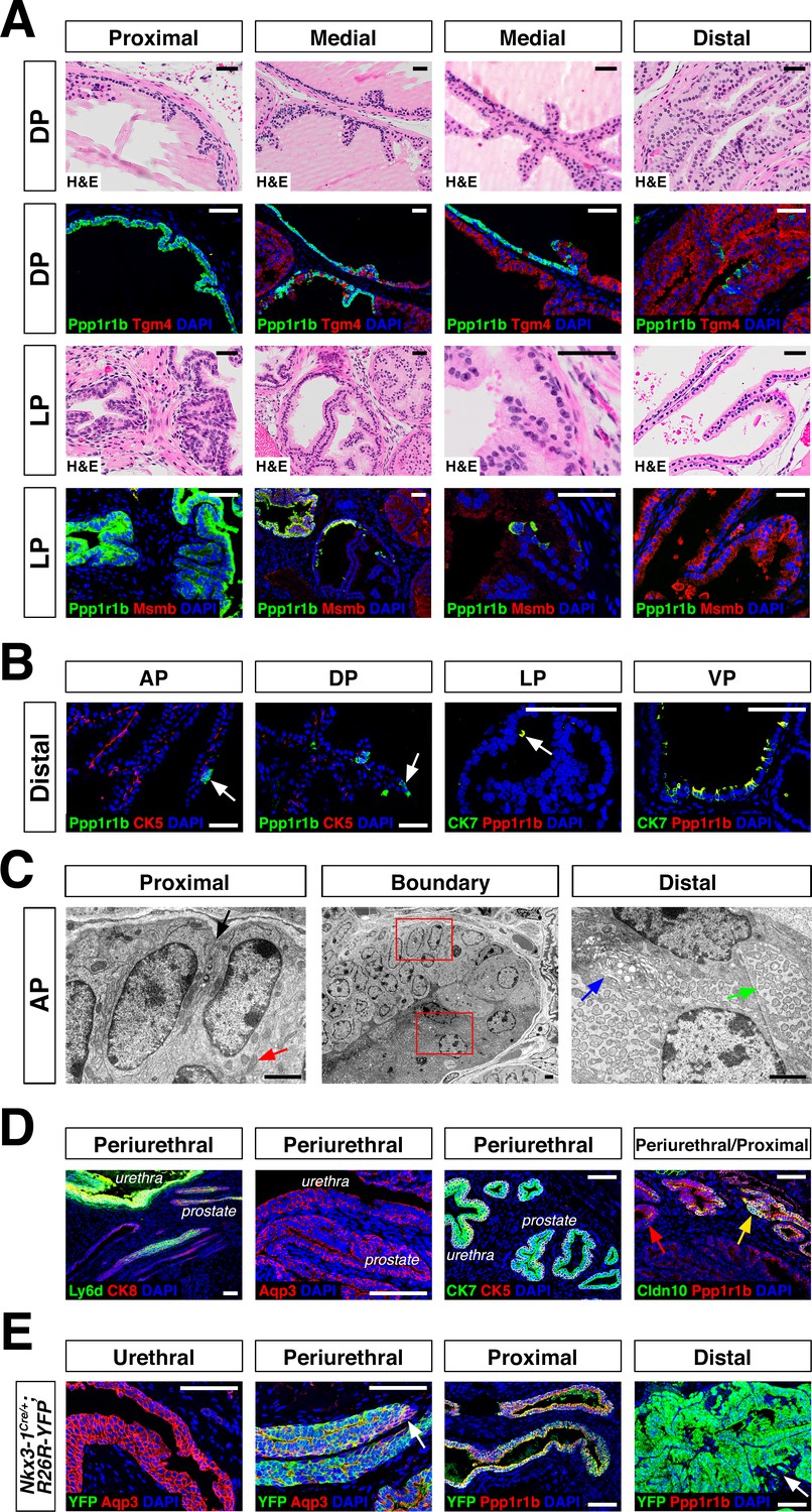
Luminal epithelial populations display spatial and morphological heterogeneity.
(A) H and E and IF of serial sections from the DP and LP, showing expression of proximal (Ppp1r1b) and distal (Tgm4, Msmb) markers; note apparent differences in the boundary regions of the two lobes. (B) Detection of distally localized LumP cells (arrows) in all four lobes; these are most abundant in the VP. (C) Scanning electron micrographs of the boundary region of the AP; central low-power image is flanked by high-power images of boxed regions. Red arrow, mitochondria; black arrow, membrane interdigitation; blue arrow, Golgi apparatus; green arrow, rough endoplasmic reticulum. (D) Identification of the periurethral region. Cells in the periurethral region generally express Ly6d, Ck7, Aqp3, and Ppp1r1b; notably, Cldn10-expressing LumP cells decrease approaching the periurethral region (E) Lineage-marking in Nkx3.1Cre/+; R26R-YFP mice (n = 3) shows widespread YFP expression in the periurethral, proximal, and distal AP; small patches remain unrecombined and lack YFP (arrows). Scale bars in (A,B,D,E) indicate 50 µm; scale bars in (C) indicate 2 µm.
Figure 2—figure supplement 1
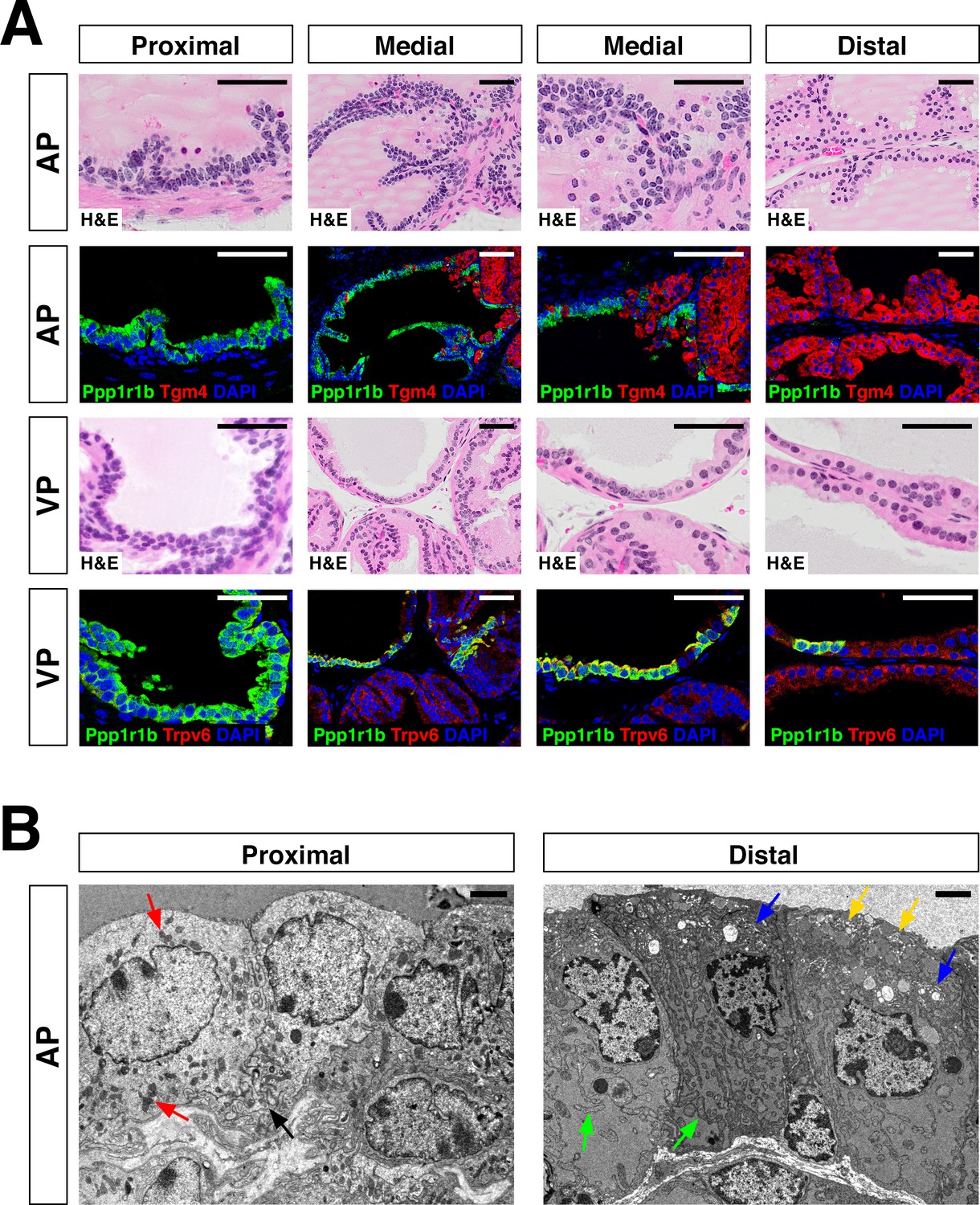
Additional analysis of proximal-distal heterogeneity.
(A) H and E and IF of serial sections from the AP and VP, showing expression of proximal (Ppp1r1b) and distal (Tgm4, Trpv6) markers. (B) Scanning electron micrographs of proximal and distal regions of the AP. Left: red arrows, mitochondria; black arrow, membrane interdigitation; Right: blue arrows, Golgi apparatus; green arrows, rough endoplasmic reticulum; yellow arrows, secretory vesicles near the apical surface. Scale bars in (A) indicate 50 µm; scale bars in (B) indicate 2 µm.
Figure 3 with 2 supplements
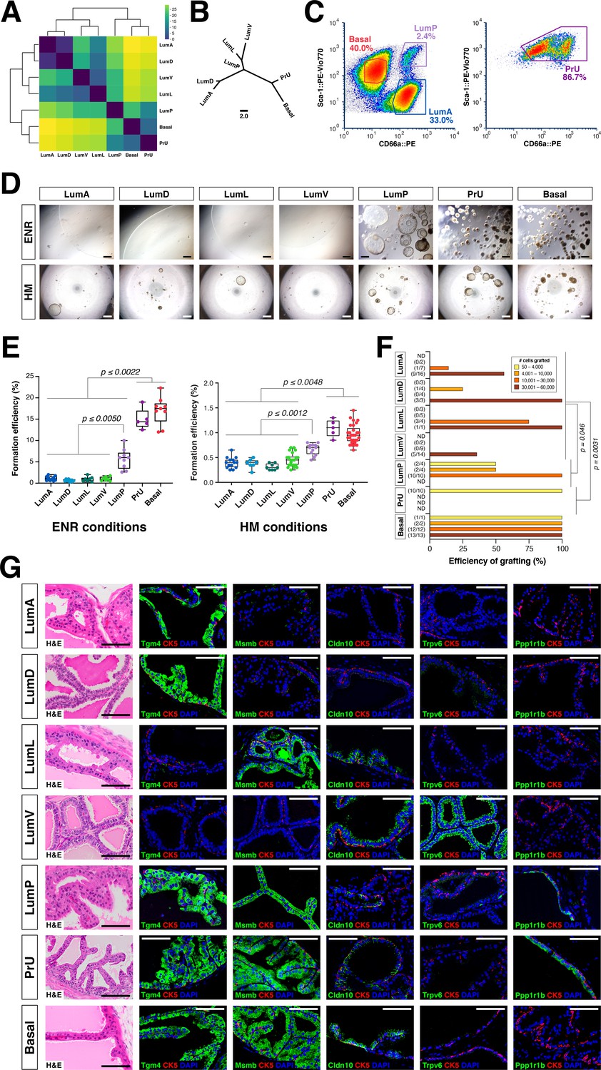
Functional analysis of epithelial populations in organoid and tissue reconstitution assays.
(A) Heatmap visualization of the Wasserstein distances between epithelial populations with hierarchical clustering. (B) Tree visualization of Wasserstein distances. (C) Flow sorting of distinct epithelial populations from the AP lobe. (D) Organoids grown from sorted epithelial cells in two distinct culture conditions. ENR conditions: sorted cells from UBC-GFP mice plated at 1000 cells/well, imaged at day 10. Hepatocyte Media (HM) conditions: sorted cells from wild type C57BL/6 mice plated at 2000-5000 cells/well and imaged on day 12-13. (E) Organoid formation efficiency plots. Maximum p-values for each pair-wise comparison are indicated. (F) Grafting efficiency in tissue reconstitution assays (average p-value shown). LumP, PrU, and basal are significantly more efficient at generating grafts from smaller number of cells relative to distal luminal populations. (G) H&E and IF of sections from fully-differentiated renal grafts; positive staining corresponds to results found in independent grafts. Scale bars indicate 50 µm.
Figure 3—figure supplement 1
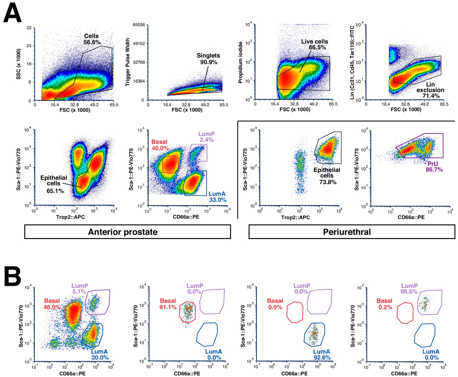
Flow-sorting strategy and validation.
(A) Sorting strategy to isolate epithelial populations from each prostate lobe. Periurethral regions were removed by dissection and sorted separately. Note that basal cells in the LP and VP are not captured efficiently by this approach. (B) Representative re-sort experiment (n = 3) to confirm purity of isolated epithelial populations.
Figure 3—figure supplement 2
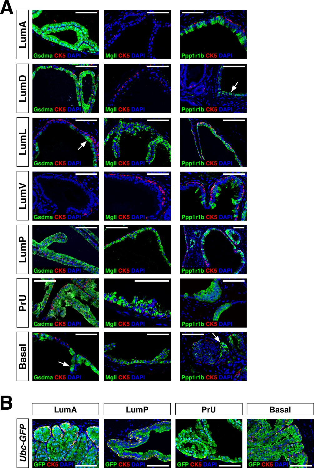
Additional marker analysis of renal grafts.
(A) Immunofluorescence staining of grafts using the indicated markers; arrows indicate regions of patchy expression. The left-most two columns show fully-differentiated graft regions, whereas the right-most column shows less-differentiated regions that are relatively small, have less abundant basal cells, are typically found on the periphery of the graft, and have fewer secretions. These less-differentiated regions tend to express the LumP marker Ppp1r1b. (B) Immunofluorescence detection of GFP in grafts from UBC-GFP mice demonstrates donor origin of grafted epithelial cells.
Figure 4 with 1 supplement
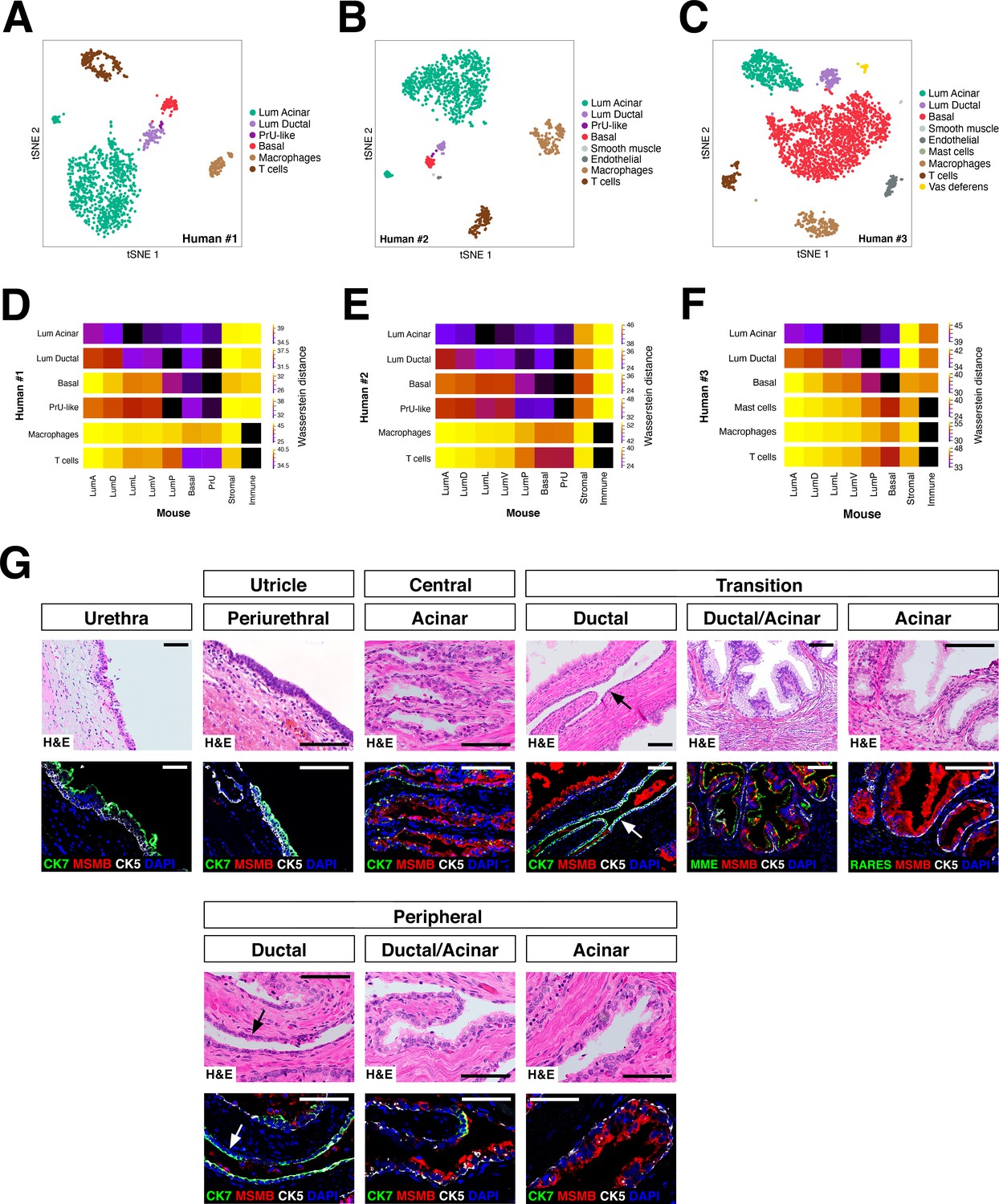
Heterogeneity and conservation of luminal populations in the human prostate.
(A–C) tSNE plot of scRNA-seq data (A, 1600 cells; B, 2303 cells; C, 2825 cells) from three independent human prostatectomy samples. (D–F) Heatmap visualization of Wasserstein distances between the human and mouse prostate populations for each dataset. (G) H and E and IF images of serial sections from human prostate, showing regions of the prostatic utricle, central, transition, and peripheral zones. Arrows indicate regions of ductal morphology. Scale bars indicate 50 µm.
-
Figure 4—source data 1
Human prostate samples and corresponding clinical data.
- https://cdn.elifesciences.org/articles/59465/elife-59465-fig4-data1-v2.docx
Figure 4—figure supplement 1
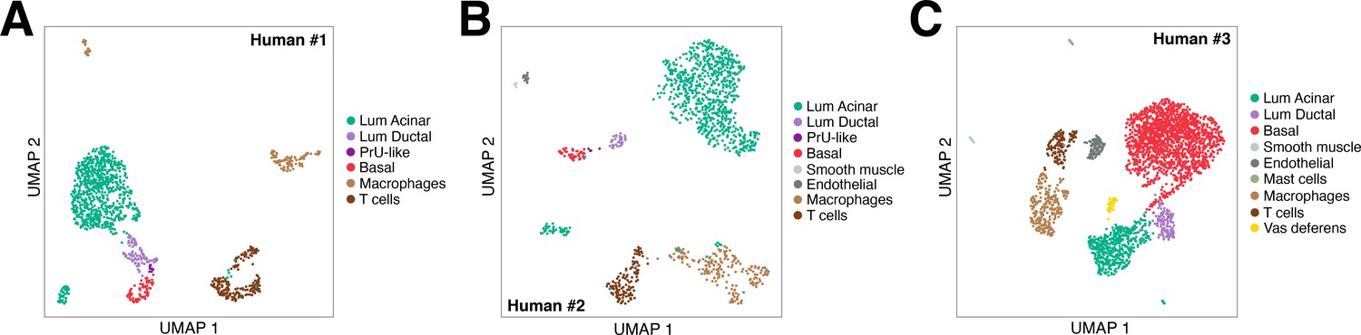
UMAP plots of human single-cell RNA-seq data.
UMAP plots are shown for three independent human prostate datasets, corresponding to the tSNE plots in Figure 4A–C.
Tables
Key resources table
| Reagent type (species) or resource | Designation | Source or reference | Identifiers | Additional information |
|---|---|---|---|---|
| Strain, strain background (Mus musculus) | C57BL/6N (wild type) | Taconic | C57BL/6NTac | 8- to 10-week-old males |
| Strain, strain background (Mus musculus) | SW (wild type) | Taconic | Tac:SW | 8- to 10-week-old males |
| Strain, strain background (Mus musculus) | UBC-GFP | Jackson Laboratory, JAX #004353 | C57BL/6-Tg(UBC-GFP) 30Scha/J | BL6 background, 8- to 13- week-old males |
| Strain, strain background (Mus musculus) | R26R-YFP | Jackson Laboratory, JAX #007903 | B6.Cg–Gt(ROSA) 26Sortm3(CAG−EYFP)Hze/J | 8- to 13-week-old males |
| Strain, strain background (Mus musculus) | Nkx3-1Cre | Shen lab | BL6 background, 8- to 13- week-old males | |
| Strain, strain background (Mus musculus) | R2G2 | Envigo | B6;129- Rag2tm1Fwa Il2rgtm1Rsky/DwIHsd | 8- to 15-week-old males |
| Strain, strain background (Mus musculus) | NOD/SCID | Jackson Laboratory, JAX #001303 | NOD.Cg-Prkdcscid/J | 8- to 15-week-old males |
| Strain, strain background (Rattus norvegicus domestica) | Sprague-Dawley embryos | Charles River #400 | SAS Sprague Dawley | E18 embryos from pregnant females |
| Antibody | Anti-mouse Cd66a (CEACAM1)-PE (recombinant monoclonal) | Miltenyi | cat 130-106-209, lot 5190208411, clone REA410 | FACS (1:700) |
| Antibody | Anti-mouse Trop-2 (Tacstd2)-APC (goat polyclonal) | R and D | cat FAB1122A, lot AAZB0117091 | FACS (1:200) |
| Antibody | Anti-mouse Sca-1 (Ly-6a/e) PE-Vio770 (recombinant monoclonal) | Miltenyi | cat 130-106-258, lots 5190308494 and 5180615495, clone REA422 | FACS (1:700) |
| Antibody | Anti-mouse Cd31 (Lin)-FITC (rat monoclonal) | eBiosciences | cat 11-0311-82, lot 1978184, clone 390 | FACS (1:700) |
| Antibody | Anti-mouse Cd45 (Lin)-FITC (rat monoclonal) | eBiosciences | cat 11-0451-82, lot 2015744, clone 30-F11 | FACS (1:700) |
| Antibody | Anti-mouse Ter119 (Lin)-FITC (rat monoclonal) | eBiosciences | cat 11-5921-82, lot 2009756, clone TER-119 | FACS (1:700) |
| Antibody | Anti-mouse Ly6d -APC-Vio770 (recombinant m onoclonal) | Miltenyi | cat 130-115-315, lot 5190715088, clone REA A906 | FACS (1:700); IF (1:100) |
| Antibody | Anti-mouse Ppp1r1b (DARPP-32) (mouse monoclonal) | SCBT | cat sc-271111, lot C2719, clone H-3 | IF (1:50) |
| Antibody | Anti-mouse Ppp1r1b (DARPP-32) (rabbit monoclonal) | Invitrogen | cat MA5-14968, lot VB2947074 | IF (1:400) |
| Antibody | Anti-mouse Trpv6 (rabbit polyclonal) | Alomone labs | cat ACC-036, lot ACC036AN1002 | IF (1:100) |
| Antibody | Anti-mouse Lrrc26 (rabbit polyclonal) | Alomone labs | cat APC-070, lot APC070AN0102 | IF (1:100) |
| Antibody | Anti-mouse Msmb (rabbit polyclonal) | Abclonal | cat A10092, lot 204440101 | IF (1:100) |
| Antibody | Anti-mouse Cldn10 (rabbit polyclonal) | Invitrogen | cat 38–8400, lot UA279882 | IF (1:100) |
| Antibody | Anti-mouse Mgll (rabbit polyclonal) | Invitrogen | cat PA5-27915, lots TI2636340A and VB2935243A | IF (1:250) |
| Antibody | Anti-mouse Tgm4 (rabbit polyclonal) | Invitrogen | cat PA5-42106, lot uc2737144 | IF (1:100) |
| Antibody | Anti-mouse Gsdma (rabbit monoclonal) | Abcam | cat ab230768, lot GR3212791-1 | IF (1:100) |
| Antibody | Anti-mouse Krt7 (rabbit monoclonal) | Abcam | cat ab68459, lot GR40294-6 | IF (1:250–500 uL) |
| Antibody | Anti-mouse Aqp3 (rabbit polyclonal) | Biorbyt | cat orb47955, lot B3440 | IF (1:500) |
| Antibody | Anti-mouse Krt5 (chicken polyclonal) | Biolegend | cat 905901, lot B271562 | IF (1:500) |
| Antibody | Anti-mouse p63 (rabbit polyclonal) | Biolegend | cat 619002, lot B262186 | IF (1:250) |
| Antibody | Anti-mouse Krt8/18 (rat monoclonal) | DSHB | Troma-1 | (1:250, lot-specific) |
| Antibody | Anti-mouse Synaptophysin (mouse monoclonal) | BD Biosciences | cat BD611880, lot 8290534 2 | IF (1:500) |
| Antibody | Anti-mouse Chromogranin A (rabbit polyclonal) | Abcam | cat ab15160, lot GR3205971-2 | IF (1:500) |
| Antibody | Anti-GFP (chicken polyclonal) | Abcam | cat ab13970, lot GR3190550-30 | IF (1:1000) |
| Antibody | Anti-mouse Nkx3.1 (rabbit polyclonal) | Athena Enzymes | cat 0315, lot 20316 | IF (1:100) |
| Antibody | Anti-mouse Ki67 (rabbit polyclonal) | Abcam | cat ab15580, lot GR3198158 | IF (1:100) |
| Antibody | Anti-mouse Krt4 (mouse monoclonal) | Invitrogen | cat MA1-35558, lot TB2524522 | IF (1:100) |
| Antibody | Anti-mouse Clusterin (rabbit polyclonal) | LS-Bio | cat LS-331486, lot 115142 | IF (1:100) |
| Antibody | Anti-mouse Wfdc2 (rabbit polyclonal) | Invitrogen | cat PA5-80226, lot TK2671201 | IF (1:100) |
| Antibody | Anti-mouse Ar (Androgen receptor) (rabbit monoclonal) | Abcam | cat ab133273, lot GR3271456-1 | IF (1:100) |
| Antibody | Anti-human Krt7 (mouse monoclonal) | Thermo Fisher | cat MA1-06316, lot OVTL12/30 | IF (1:200) |
| Antibody | Anti-human Rarres1 (mouse monoclonal) | Thermo Fisher | cat MA5-26247, lot OTI1D2 | IF (1:200) |
| Antibody | Anti-human Cd10 (Mme) (mouse monoclonal) | SCBT | cat sc-46656, clone F-4 | IF (1:100) |
| Antibody | Anti-human Msmb (rabbit polyclonal) | Abclonal | cat A10092 | IF (1:200) |
| Software, algorithm | Random Matrix Theory | R. Rabadan Lab | https://rabadan.c2b2.columbia.edu /html/randomly/ | |
| Software, algorithm | Python Optimal Transport | Rémi Flamary and Nicolas Courty, POT Python Optimal Transport library | https://github.com/rflamary/POT | |
| Software, algorithm | Phylogenetic tree analysis | Phangorn package | https://github.com/ KlausVigo/phangorn | |
| Software, algorithm | Leiden algorithm | F. A. Wolf, P. Angerer, and F. J. Theis, Genome Biology (2018). ‘SCANPY: large-scale single-cell gene expression data analysis’ | https://scanpy. readthedocs.io/en/stable |
Additional files
Download links
A two-part list of links to download the article, or parts of the article, in various formats.
Downloads (link to download the article as PDF)
Open citations (links to open the citations from this article in various online reference manager services)
Cite this article (links to download the citations from this article in formats compatible with various reference manager tools)
A single-cell atlas of the mouse and human prostate reveals heterogeneity and conservation of epithelial progenitors
eLife 9:e59465.
https://doi.org/10.7554/eLife.59465


