Cryo-EM reveals species-specific components within the Helicobacter pylori Cag type IV secretion system core complex
- Department of Pathology, Microbiology, and Immunology, Vanderbilt University Medical Center, United States
- Life Sciences Institute, University of Michigan, United States
- Department of Medicine, Vanderbilt University School of Medicine, United States
- Veterans Affairs Tennessee Valley Healthcare System, United States
- Department of Cell and Developmental Biology, University of Michigan, United States
Figures
Figure 1 with 4 supplements
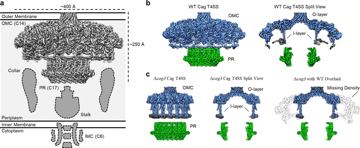
Comparison between maps of the wild-type (WT) and ΔCag3 Cag T4SS core complex.
(a) The Cag T4SS spans the inner membrane and outer membrane and consists of distinct features with differing symmetry: the OMC (C14 symmetry), the PR (C17 symmetry), an inner-membrane complex (IMC, C6 symmetry), and the stalk and collar with unknown symmetries. (b) In the reconstruction of the WT Cag T4SS, we observe the O-layer of the OMC (shown in blue), the I-layer of the OMC (shown in gray), and the PR (shown in green). Left panel, WT Cag T4SS density map; Right panel, central slice of the WT density map. (c) All of these features are observed in the ΔCag3 Cag T4SS map (shown in the same colors as panel b), but peripheral regions of the OMC are missing in the ΔCag3 Cag T4SS map (shown in white). Left panel, ΔCag3 Cag T4SS density map; middle panel, central slice of ΔCag3 Cag T4SS density map; right panel, overlaid central slices of WT (grey) and ΔCag3 (blue and green) Cag T4SS density maps.
Figure 1—figure supplement 1
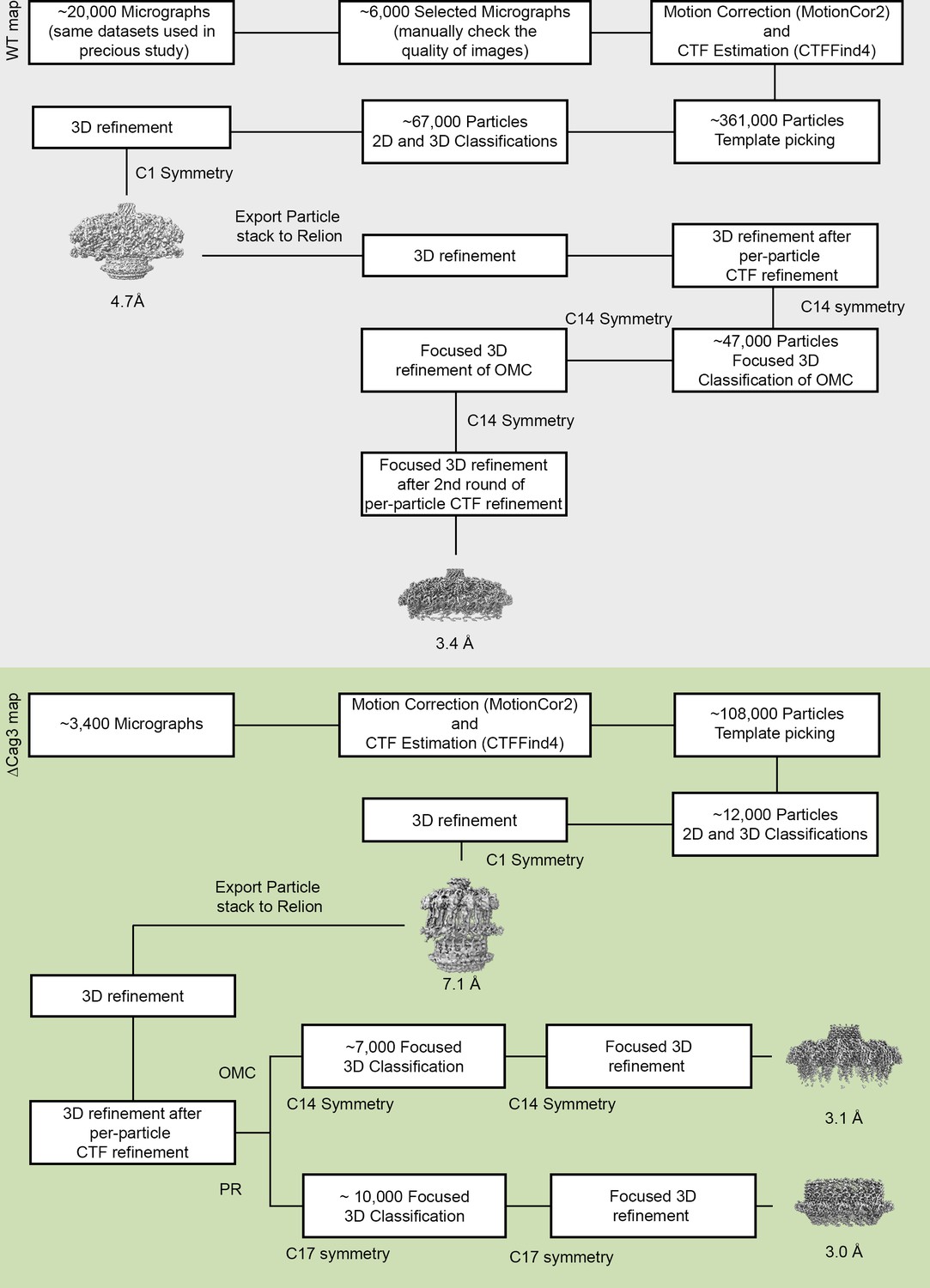
Flow chart of cryo-EM processing steps.
The processing steps for WT Cag T4SS data are on a gray background and the processing steps for ΔCag3 Cag T4SS data are on a green background. All the raw micrographs used in the WT Cag T4SS 3D reconstructions were identical to the datasets used in our previous study (Chung et al., 2019). Approximately 6000 high quality images were selected from ~20,000 images.~361,000 particles were selected by template picking in CryoSPARC. After 2D and 3D classification, the best class (~67,000 particles) was chosen for further refinement, without symmetry (C1). All the particles used in the 3D refinement of CryoSPARC were exported into RELION for further steps and the 4.7 Å 3D model with C1 symmetry was filtered to 60 Å resolution and used as an initial model for 3D structure determination in RELION. Focused 3D classification and 3D refinement were used to determine higher resolution maps of the WT OMC (with 14-fold symmetry), resulting in a 3D map of the OMC (14-fold symmetry) at 3.4 Å. Similar steps were applied to ΔCag3 Cag T4SS data. Approximately 3400 micrographs were collected and ~108,000 particles were selected by template picking in CryoSPARC. After the 2D/3D filtration and further refinement (3D map at 7.1 Å with C1 symmetry),~12,000 particles were exported into RELION for further steps. Focused 3D classification (without alignment) was used to determine higher resolution maps of the ΔCag3 OMC (with 14-fold symmetry) and the PR (with 17-fold symmetry). The maps of the OMC and PR were further refined using focused 3D refinement (with local refinement), resulting in 3D maps of the OMC (14-fold symmetry) and the PR (17-fold symmetry) at 3.1 Å and 3.0 Å, respectively.
Figure 1—figure supplement 2
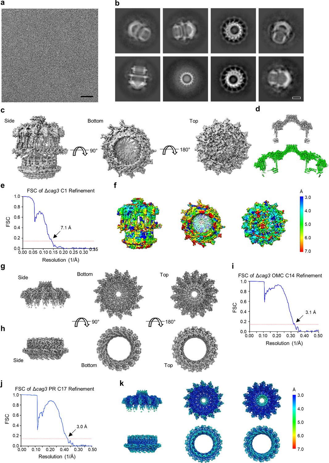
Cryo-EM processing of the ΔCag3 Cag T4SS core complex.
(a) Sub-area of a motion-corrected image of vitrified ΔCag3 Cag T4SS particles. Scale bar, 50 nm. (b) Selected 2D class averages. Scale bar, 10 nm. (c) Rotated views of the 3D reconstructed model with no applied symmetry (C1, 7.1 Å resolution). (d) A comparison between maps of the ΔCag3 (gray) and WT (green) OMC. (e) FSC of C1 refinement after applying a tight mask in cryoSPARC. Dotted red line, Fourier Shell Correlation (FSC) = 0.143. (f) Heat map showing local resolution of C1 3D reconstruction. The heat map scales are exponential. (g) Views of the focused refined 3D model of the ΔCag3 OMC with C14 symmetry applied (3.1 Å resolution) and (h) ΔCag3 PR with C17 symmetry applied (3.0 Å resolution). (i) FSC of focused ΔCag3 C14 OMC and (j) ΔCag3 C17 PR refinements. Dotted red line, FSC = 0.143. (k) Map of local resolution of focused ΔCag3 C14 OMC and ΔCag3 C17 PR refinement. The heat map scales are exponential.
Figure 1—figure supplement 3
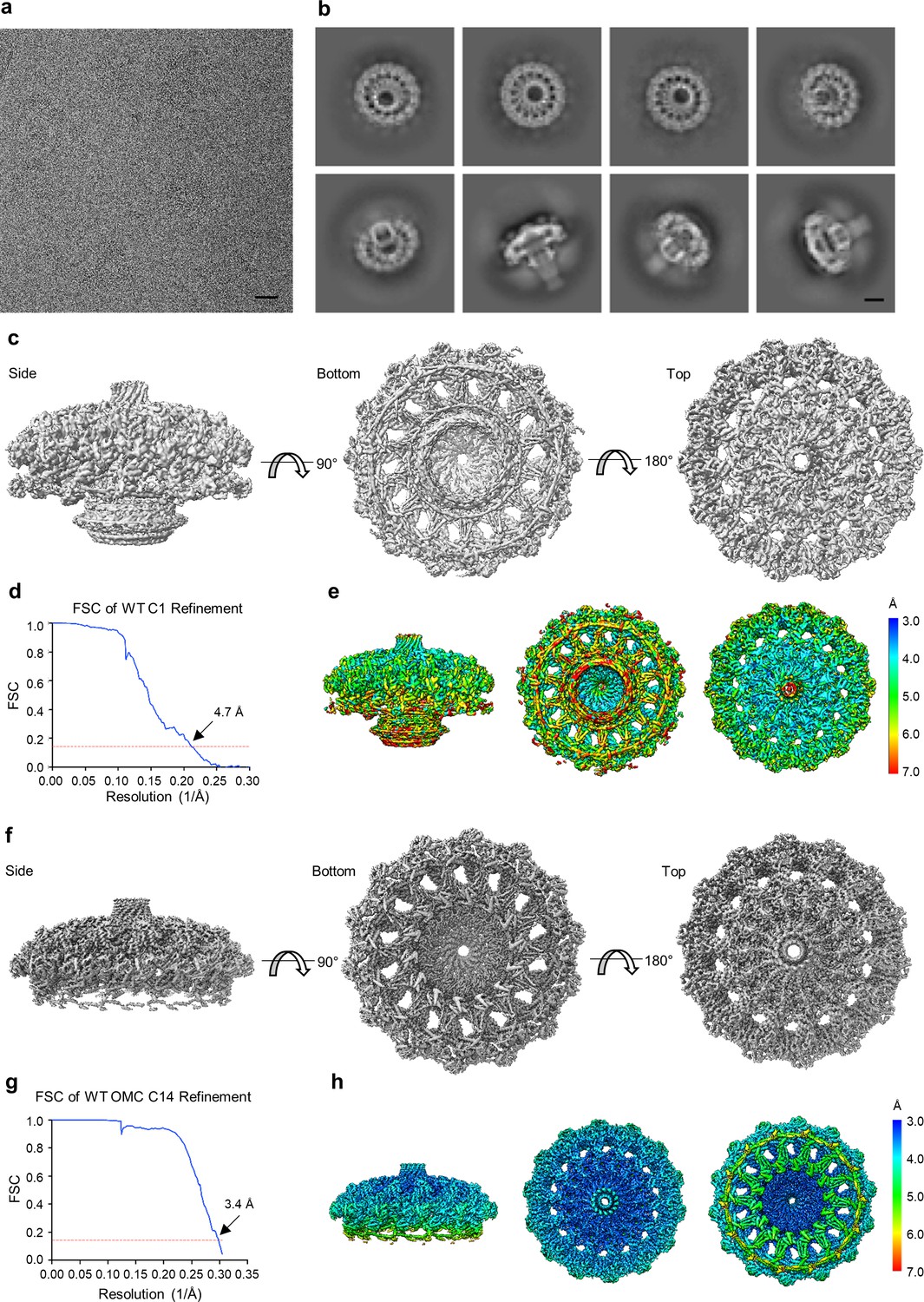
Cryo-EM processing of the WT Cag T4SS core complex.
(a) Sub-area of a motion-corrected image of vitrified WT Cag T4SS particles. Scale bar, 50 nm. (b) Selected 2D class averages. Scale bar, 10 nm. (c) Rotated views of the 3D reconstructed model of the WT Cag T4SS with no applied symmetry (C1, 4.7 Å resolution). (d) FSC of C1 refinement after applying a tight mask in cryoSPARC. Dotted red line, Fourier Shell Correlation (FSC) = 0.143. (e) Heat map showing local resolution of C1 3D reconstruction. The heat map scales are exponential. (f) Views of the focused refined 3D model of the WT OMC with C14 symmetry applied (3.4 Å resolution). (g) FSC of focused C14 OMC refinement. Dotted red line, FSC = 0.143. (h) Map of local resolution of focused WT OMC refinement. The heat map scales are exponential.
Figure 1—figure supplement 4
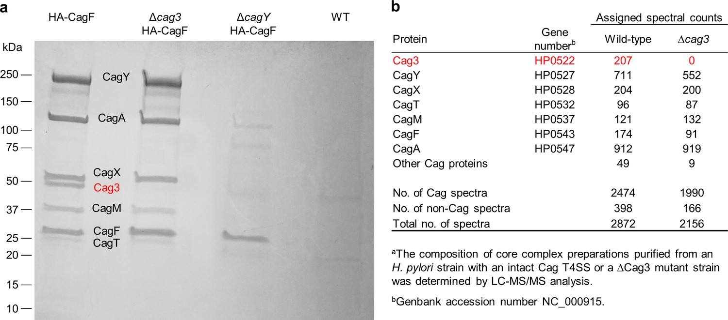
Analysis of Cag T4SS core complex preparations.
(a) SDS-PAGE analysis of core complexes purified from wild-type and Δcag3 H. pylori strains, each producing HA-tagged CagF (first and second lanes). The same purification methods were applied to a ΔcagY mutant strain producing HA-tagged CagF (defective in core complex assembly) or a control wild-type strain with no modification of CagF. Dominant bands visible in the first lane have molecular masses consistent with CagY (219 kDa), CagA (132 kDa), CagX (61 kDa), Cag3 (55 kDa), CagM (44 kDa), CagT (32 kDa), and CagF (32 kDa). LC-MS/MS analysis of excised bands confirmed these identifications. The 55 kDa band (indicated in red) is absent from the ΔCag3 mutant core complex preparation. (b) Mass spectrometric analysis of core complex samples purified from the WT and ΔCag3 H. pylori strains.
Figure 2 with 6 supplements

The asymmetric unit of the WT and ΔCag3 Cag T4SS core complex.
(a) A cross-section model of the mapped portions of CagY (yellow), CagX (orange), CagT (red and salmon), CagM (brown and tan), and Cag3 (various shades of green and blue) in the OMC from the WT Cag T4SS. Portions of CagX and CagY are present in both the OMC and the PR (denoted by the gray box). (b) A cartoon representation of the WT Cag T4SS core complex proteins, colored as in panel a. The dotted lines represent densities that were not clearly seen in the density maps. (c) A cross-section model of the mapped portions of CagY (yellow), CagX (orange), and CagT (red) from the ΔCag3 Cag T4SS core complex. (d) A cartoon representation of the ΔCag3 Cag T4SS core complex proteins with CagY (yellow), CagX (orange), CagT-1 (red). The red rectangles represent the alternate conformation of the C-terminal helices of CagT-1. CagT-2 and Cag-3 were not observed within this map. The dashed lines represent densities that were not clearly seen in the density map.
Figure 2—figure supplement 1
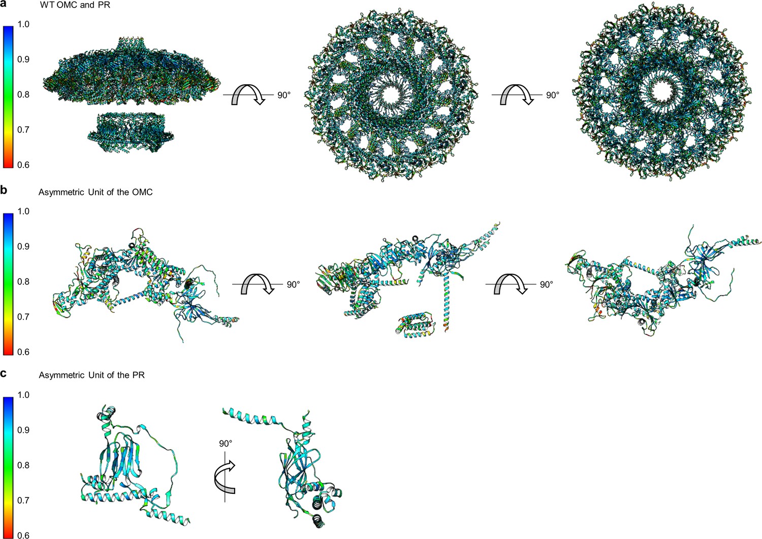
Correlation of each component of the WT Cag T4SS to experimental maps.
(a) The correlation coefficient of each residue is plotted on the structure of the entire WT Cag T4SS as a heat map. The asymmetric units of the OMC (b) and the PR (c) depict the relative quality of the models in each portion of the structure.
Figure 2—figure supplement 2
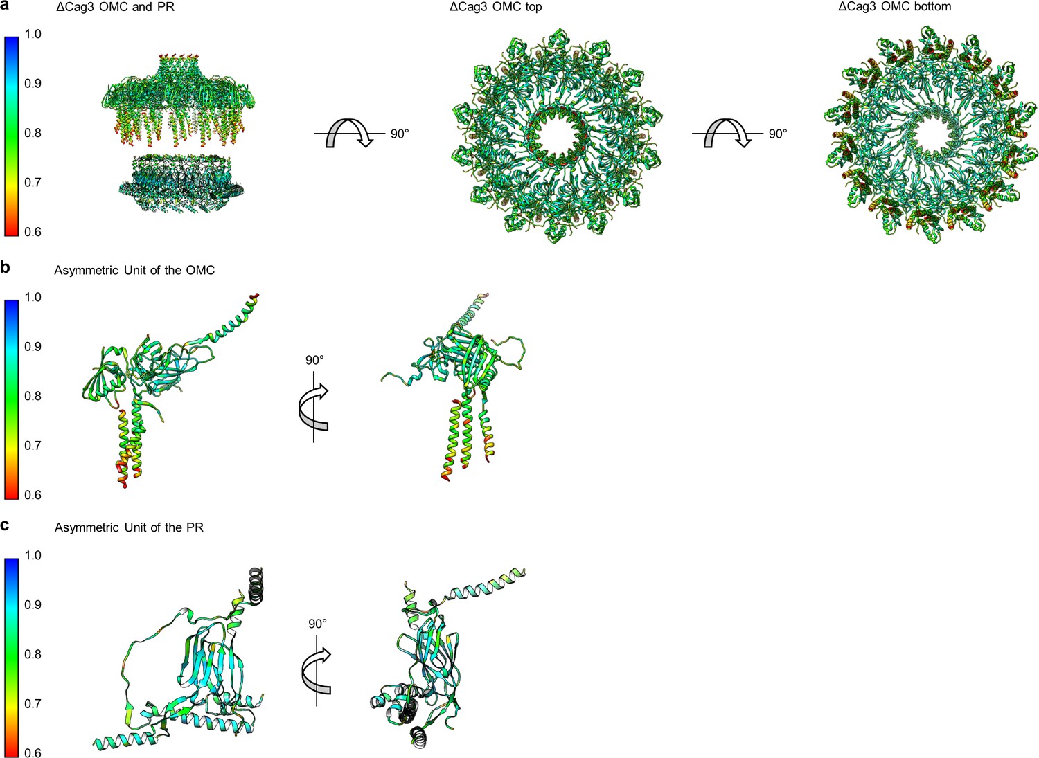
Correlation of each component of the ΔCag3 Cag T4SS to experimental maps.
(a) The correlation coefficient of each residue is plotted on the structure of the entire ΔCag3 Cag T4SS as a heat map. The OMC is rotated to show ‘top’ and ‘bottom’ views. The asymmetric units of the OMC (b) and the PR (c) depict the relative quality of the models in each portion of the structure.
Figure 2—figure supplement 3
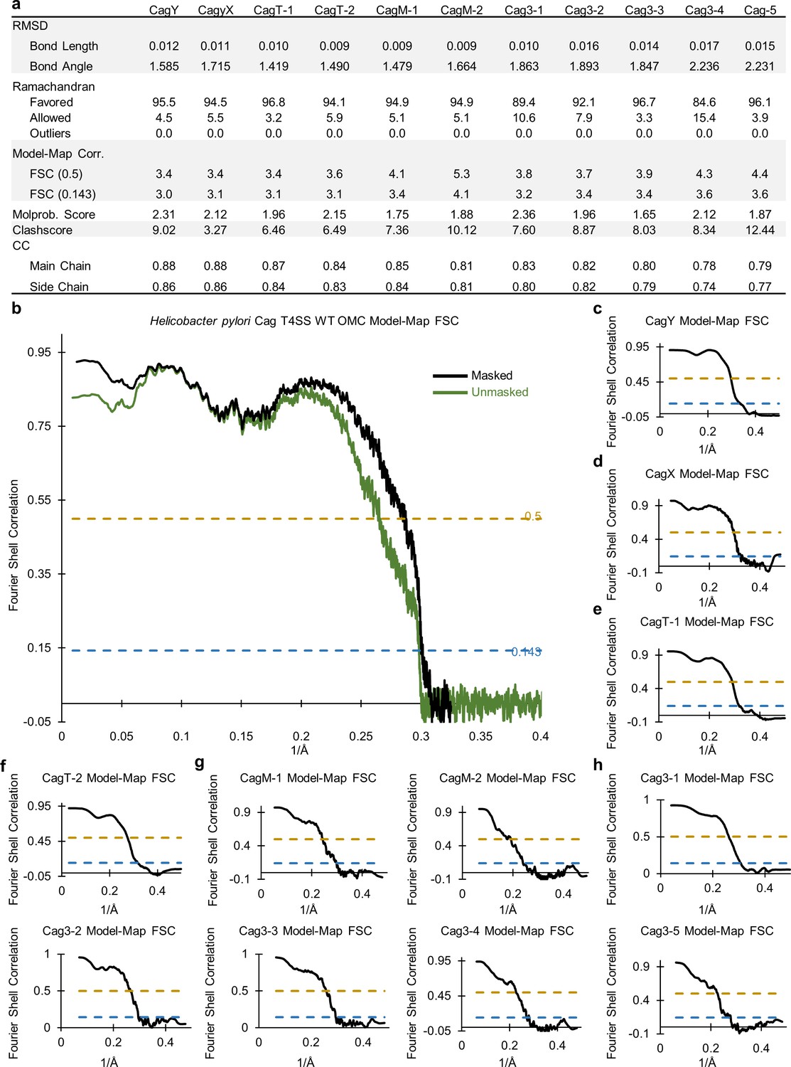
Correlation between the WT OMC cryo-EM map and models.
(a) Statistics for each of the constructed models indicate their relative quality. (b) A model-map correlation curve for the entire WT OMC is shown, with the unmasked data in green and the masked data in black. (c–h). The model-map correlation was also determined for each of the individual protein structures within the OMC.
Figure 2—figure supplement 4
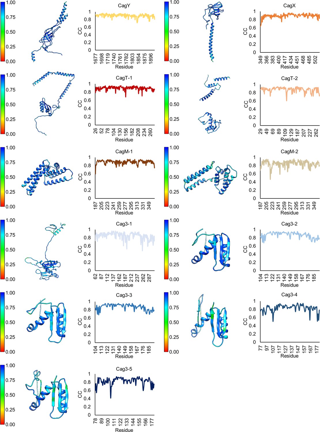
Model-map correlation for each protein within the OMC.
(a) The correlation coefficient for each protein within the OMC is depicted as a heat map on the corresponding structure and is plotted against the residue number.
Figure 2—figure supplement 5
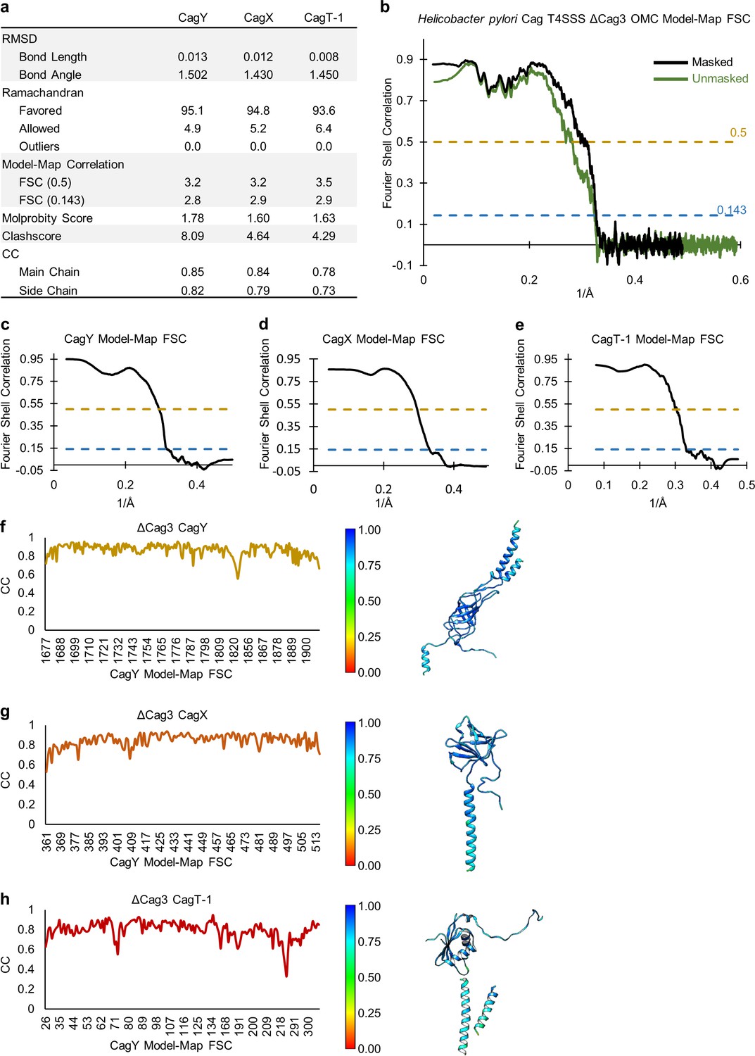
Quality of models within the OMC of the ΔCag3 T4SS.
(a) Statistical analysis for each of the models constructed within the OMC of the ΔCag3 T4SS. (b) A model-map FSC curve is shown for the OMC of the ΔCag3 T4SS. The green line indicates data derived using an unmasked map and the black line indicates data derived using a masked map. (c–e) A model-map FSC curve is shown for all models constructed in the ΔCag3 OMC map. (f–h) Per-residue correlation coefficients are plotted against residue number (left) and are depicted as a heat map on the corresponding structures (right).
Figure 2—figure supplement 6
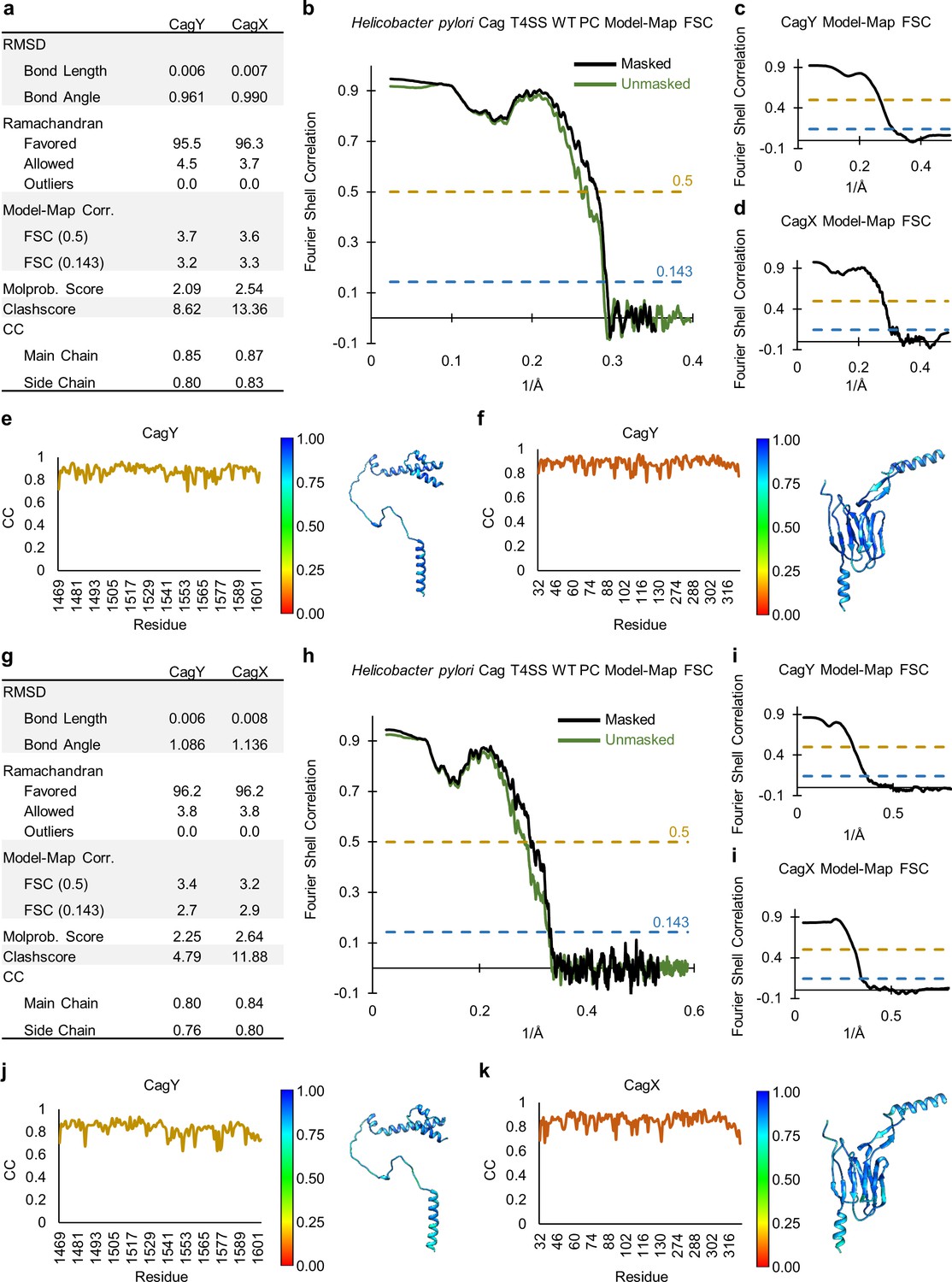
Quality of models within the PR of the WT and ΔCag3 maps.
(a) Statistical analysis of all models constructed within the PR of the WT T4SS. (b) A model-map FSC curve is shown for the PR of the WT T4SS. The green line indicates data derived using an unmasked map and the black line indicates data derived using a masked map. (c, d) A model-map FSC curve is shown for CagY and CagX. (e, f) Per-residue correlation coefficients are plotted against residue number (left) and are depicted as a heat map on the corresponding structure (right). (g) Statistical analysis of all models constructed within the PR of the ΔCag3 T4SS. (h) A model-map FSC curve is shown for the PR of the ΔCag3 T4SS. The green line indicates data derived using an unmasked map and the black line indicates data derived using a masked map. (i) A model-map FSC curve is shown for CagY and CagX. (j, k) Per-residue correlation coefficients are plotted against residue number (left) and are depicted as a heat map on the corresponding structures (right).
Figure 3
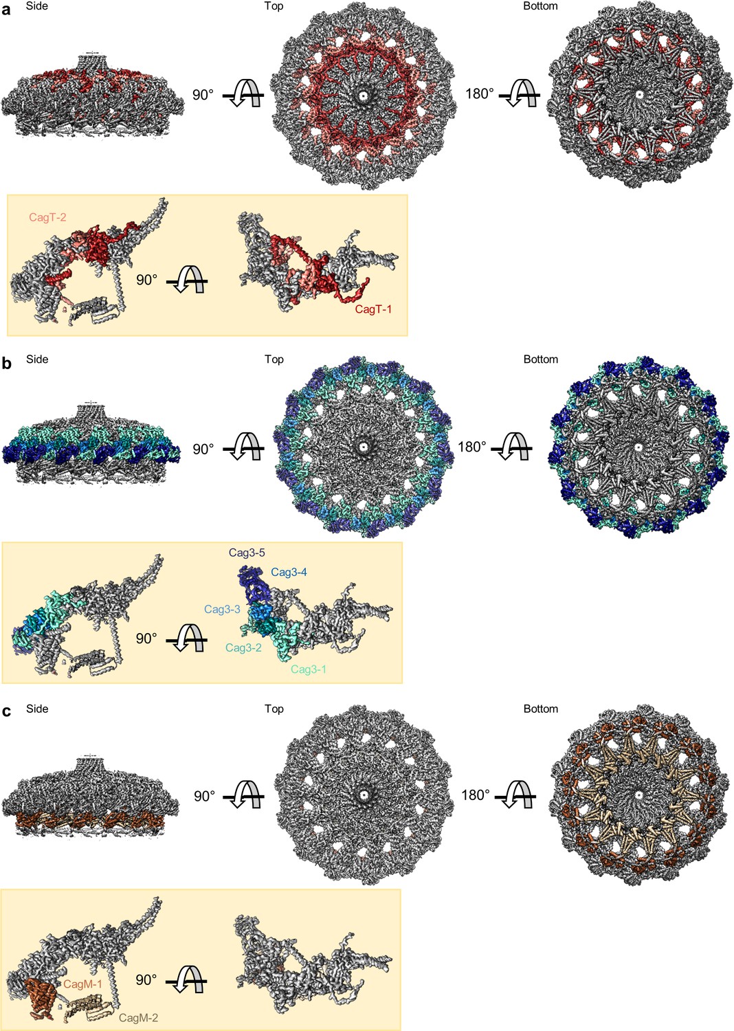
Locations of components within the OMC.
(a) The O-layer of the OMC contains two copies of CagT (CagT-1 and CagT-2) (shown in red and salmon). The two copies are localized within the center of the asymmetric unit (inset) as shown in red and salmon. (b) Cag3 comprises a significant portion of the O-layer of the Cag T4SS, as shown in blue and green. Within the asymmetric unit (inset), we observe five copies of Cag3 (denoted Cag3-1 through Cag3-5, shown in various shades of blue and green). (c) Within the I-layer of the OMC, there are two similar folds, each defined as CagM. Within the asymmetric unit, we observe two copies (inset) that are colored in brown and tan.
Figure 4 with 2 supplements
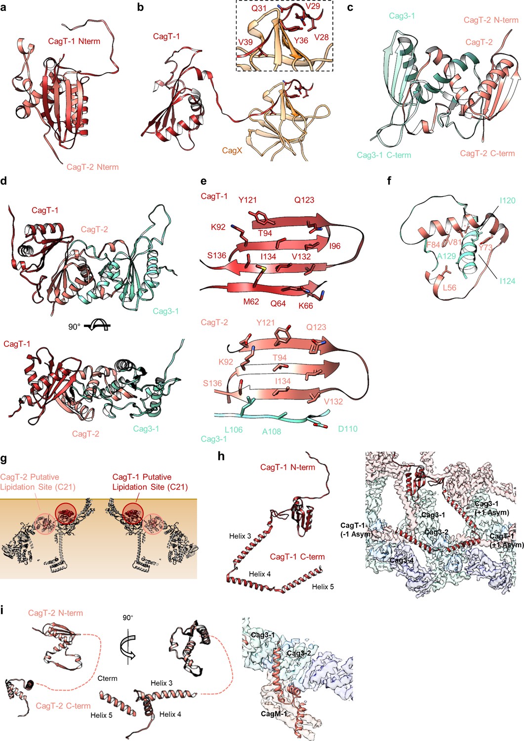
The N- and C-termini from CagT-1 and CagT-2 are positioned differently.
(a–c) The N-terminus of CagT-1 extends inward toward the center of the map and interacts with CagX from the next asymmetric unit. The residues that contribute to this interaction are largely hydrophobic, as indicated in the inset panel. CagT-2 differs from CagT-1 in that the N-terminus of the protein extends outward toward the periphery of the map, forming the last strand of a β-sheet with Cag3-1. (d) The three proteins (CagT-1, CagT-2 and Cag3-1) have an interwoven architecture. (e) The interface that is formed between the three proteins consists of two β-sheets that include strands from all three molecules. (f) The interface of CagT-2 and Cag3-1 is a pair of α-helices that bury hydrophobic residues within the interface. (g) The position of the N-terminal loops of CagT-1 (red) and CagT-2 (salmon) are such that the putative lipidation sites are near the outer membrane. (h) The C-terminal α-helices of CagT-1 adopt an extended conformation (left) and interact with Cag3-1, Cag3-2, and Cag3-4 within the same asymmetric unit and Cag3-1 and CagT-1 in neighboring asymmetric units (right). (i) The C-terminal α-helices of CagT-2 are connected by an apparently flexible linker (left) and interact with Cag3-1, Cag3-2, and CagM-1 (right).
Figure 4—figure supplement 1
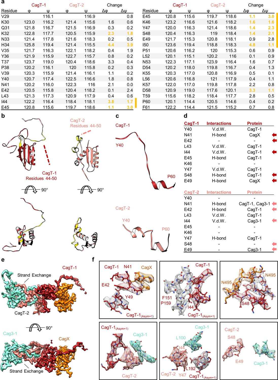
The N-terminal loop of CagT is observed in two different conformations.
(a) The dihedral angles of residues within the N-terminal loop of CagT-1 and CagT-2 are plotted. The difference between the angles was used to determine where the largest change occurred. Residues in which both the φ and ψ angles changed by >1° are highlighted in yellow. (b) The N-terminal loop of CagT-1 (red) and CagT-2 (salmon) is highlighted in yellow. (c) The residues of CagT-1 and CagT-2 that exhibited the most striking change are depicted. (d) Residues within these loops engage in protein-protein interactions with different subsets of proteins. The table lists relevant residues along with the type of interaction mediated and the interacting protein. Arrows indicate residues with different interacting partners. (e) The orientations of the N-terminal loops are shown. A loop of CagT-1 interacts with CagX and a loop of CagT-2 completes a β-sheet formed by Cag3. (f) The interactions mediated by the N-terminal loops are shown here. The top row depicts interactions mediated by the N-terminal loop of CagT-1, and the bottom row depicts interactions mediated by the N-terminal loop of CagT-2. Proteins are colored as they appear in panel (e), with proteins from adjacent asymmetric units depicted with gray density.
Figure 4—figure supplement 2
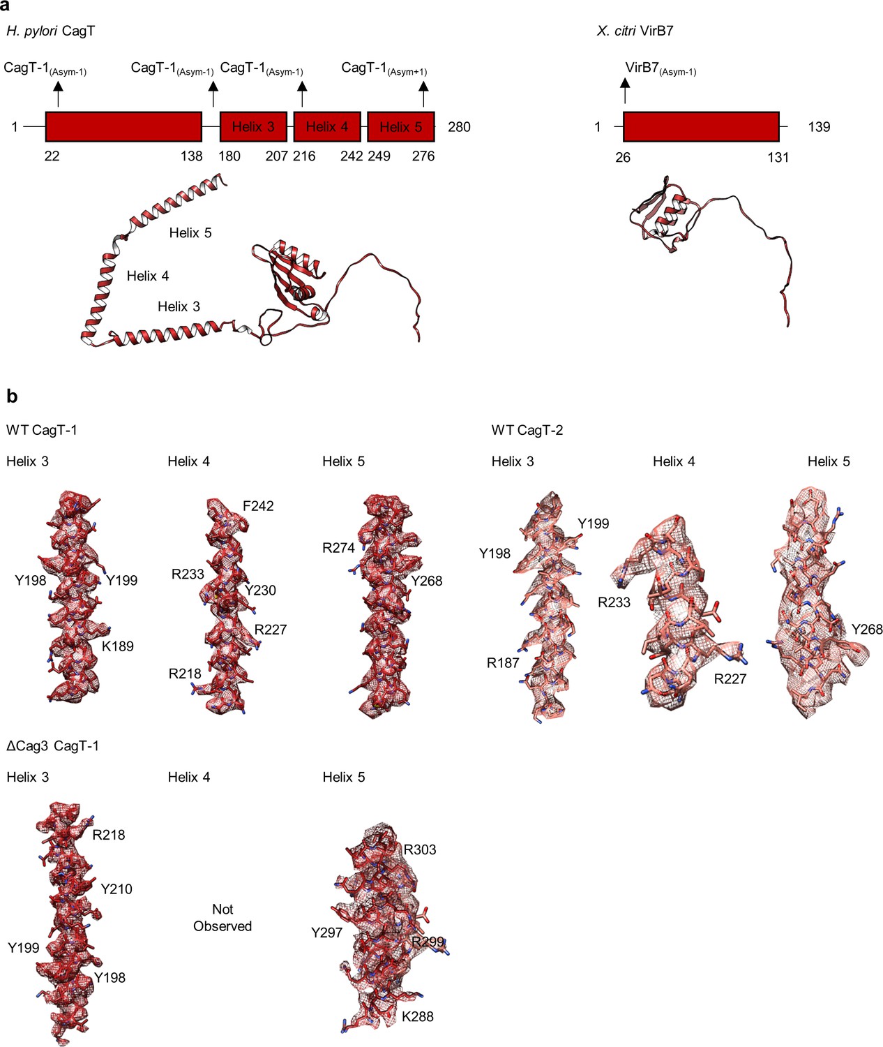
The C-terminal helices of CagT mediate interactions within the OMC.
(a) Domain diagrams of H. pylori CagT and X. citri VirB7. The two proteins have similar N-terminal domains that mediate interactions with other components in the respective T4SSs. CagT contains three additional helices within the C-terminus of the protein that mediate interactions with adjacent asymmetric units. (b) The three C-terminal helices of CagT-1 and CagT-2 observed within the WT map are shown with experimental density displayed as a mesh (top). Landmark residues demonstrating the accuracy of the register are shown. The two C-terminal helices of CagT-1 that were observed within the ΔCag3 map are shown with experimental density displayed as a mesh (bottom). Landmark residues demonstrating the accuracy of the register are shown.
Figure 5
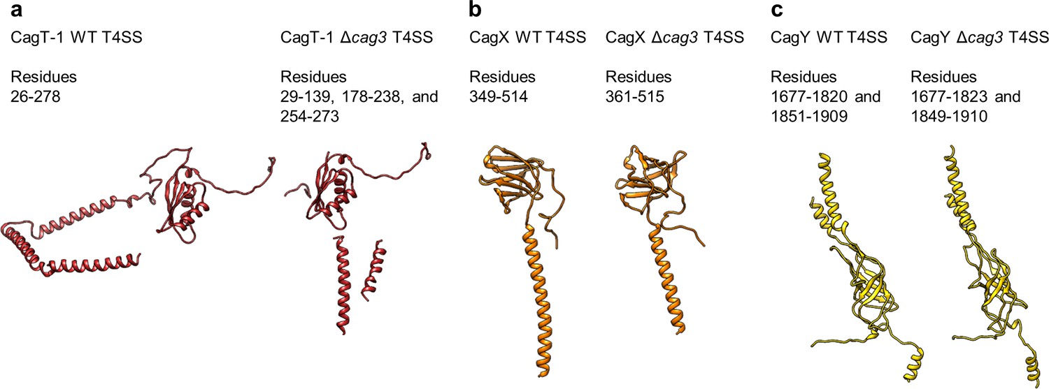
Conservation of protein structures in WT and ΔCag3 Cag T4SS complexes.
(a) Despite global differences between the overall WT and Δcag3 maps, the structure of CagT-1 shares a similar core VirB7-like fold in both maps. (b–c) Similarly, CagX and CagY adopt nearly identical orientations within both maps. The illustrated portions of CagX and CagY are the domains localized to the OMC.
Figure 6 with 1 supplement
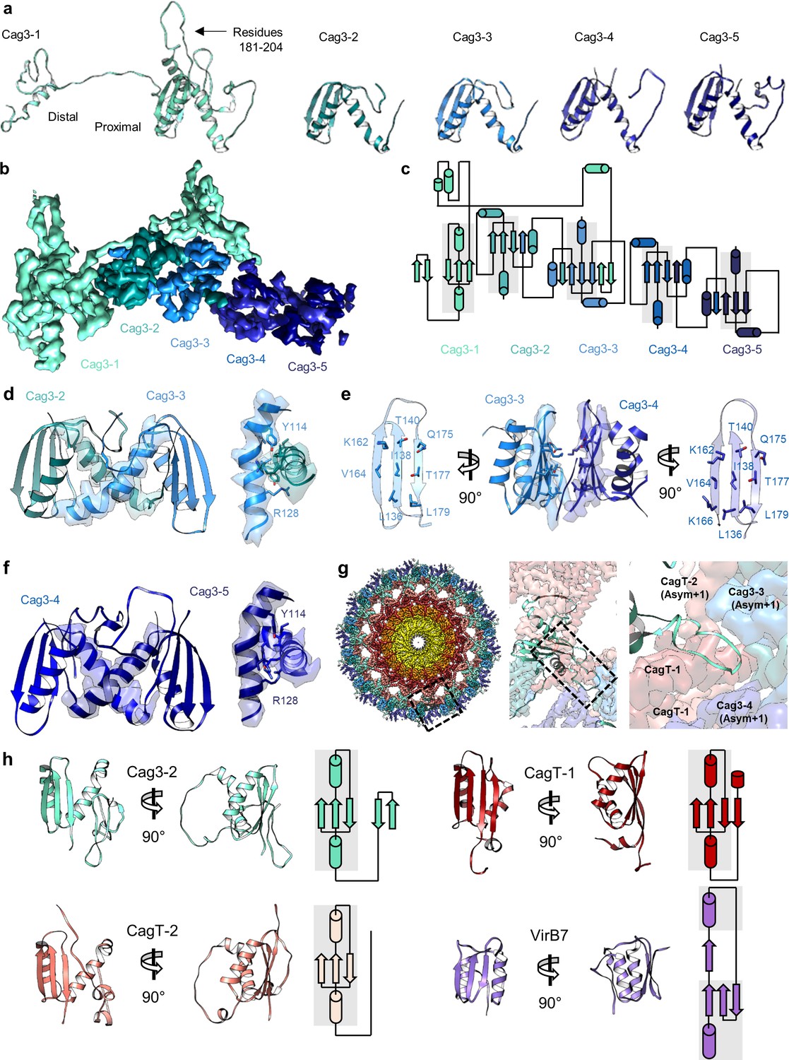
There are five copies of Cag3 within the OMC asymmetric unit.
(a) Five different molecules of Cag3 are present within the asymmetric unit. The general architecture of Cag3 can be described as two domains, the proximal domain (residues 62–232) and the distal domain (residues 252–309). (b) All five of the Cag3 proteins share a heavily interwoven architecture in which β-sheets are formed between adjacent molecules within the asymmetric unit. (c) A topology diagram showing the general architecture of all copies of Cag3 within the asymmetric unit. (d) The interface of Cag3-2 (cyan) and Cag3-3 (light blue) is formed predominantly by two helices with contact mediated by Y114 and R128 of each molecule. (e) The interface of Cag3-3 (light blue) and Cag3-4 (blue) is dramatically different from the other Cag3 interfaces and includes an extensive hydrophobic interaction that is formed by two adjacent beta sheets. (f) Cag3-4 (blue) and Cag3-5 (navy blue) share a similar interface as Cag3-2 and Cag3-3, as shown above. (g) A view of the Cag T4SS is shown from the top-down (left) and indicates the position of a loop within the Cag3-1 proximal domain (amino acids 181–204, black box) that mediates contacts between asymmetric units. (h) The proximal domain of Cag3 contains a fold that is structurally similar to folds within CagT-1 (shown in red), CagT-2 (shown in salmon) and X. citri VirB7 (PDB 6GYB, shown in purple).
Figure 6—figure supplement 1
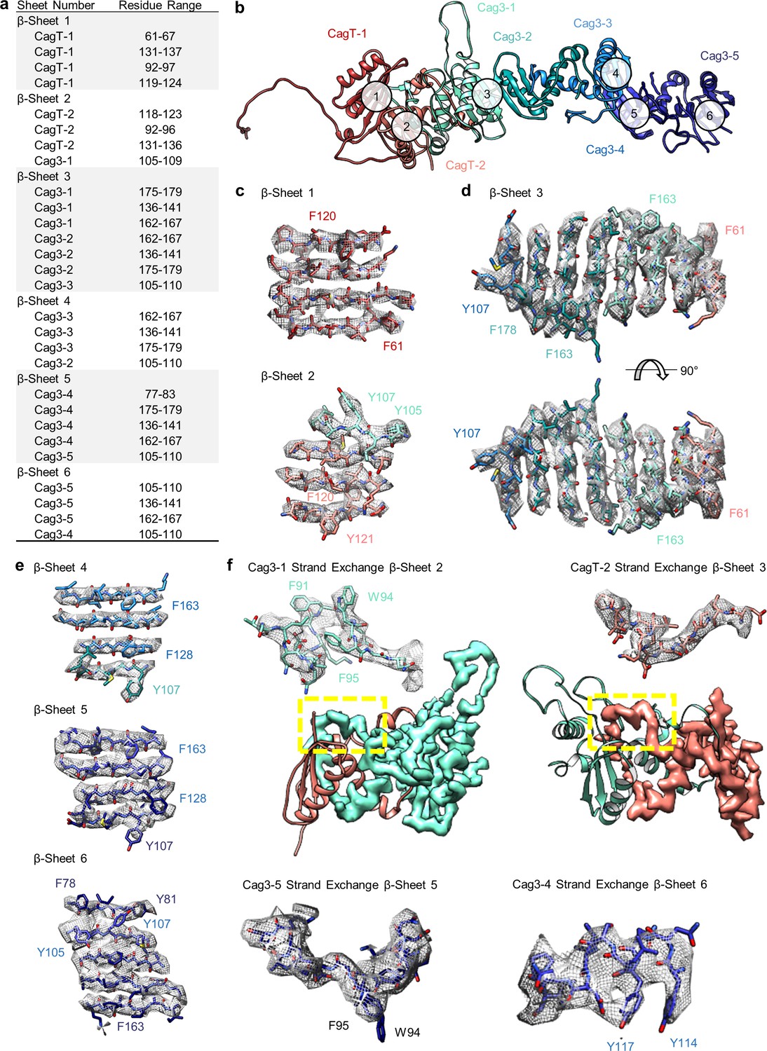
The repetitive β-sheet structure of CagT and Cag3.
(a) The table lists residues that contribute to six β-sheets formed by copies of CagT and Cag3 within the OMC. The location of these six β-sheets is indicated in panel (b). (c–e) Representative density for all β-sheets with landmark residues noted for each. (f) Representative density for β-sheet strand exchange is shown for β-sheet 3 (top, left), β-sheet 4 (top, right), β-sheet 5 (bottom, left), and β-sheet 6 (bottom, right).
Figure 7
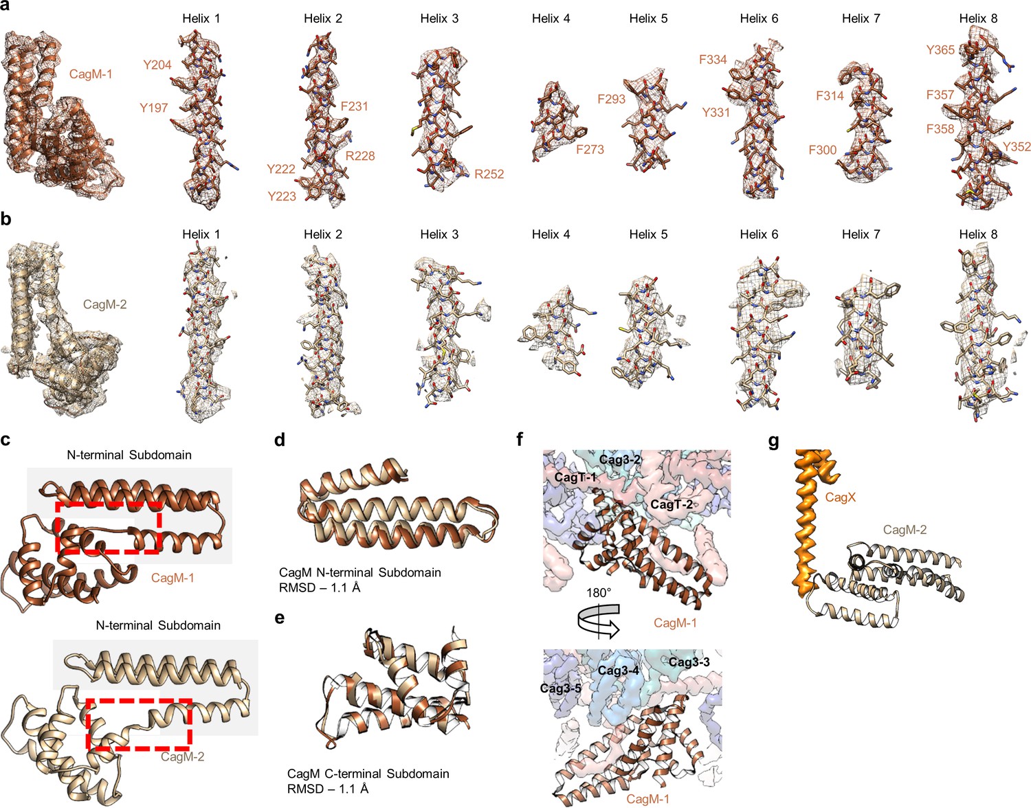
Localization of CagM within the I-layer of the OMC.
(a) We modeled a single domain of CagM-1, consisting of 8 helices within the I-layer of the OMC. Representative density for all eight helices is shown with landmark residues indicated. (b) Although the local resolution within the I-layer is notably lower than that of the O-layer, several structural features within the I-layer density are consistent with the sequence of CagM (designated CagM-1). The correlation of all 8 helices of CagM-2 to the experimental map is shown. (c) The two subdomains within CagM are connected by a hinge (noted by the red dotted line). When the CagM-1 subdomains are aligned independently, we note RMSDs of 1.1 Å for both the N-terminal subdomain (d) and the C-terminal domain (e). The differences in sub-domain orientation are likely the result of differences in interacting partners of CagM-1 (f) and CagM-2 (g) within the OMC.
Figure 8
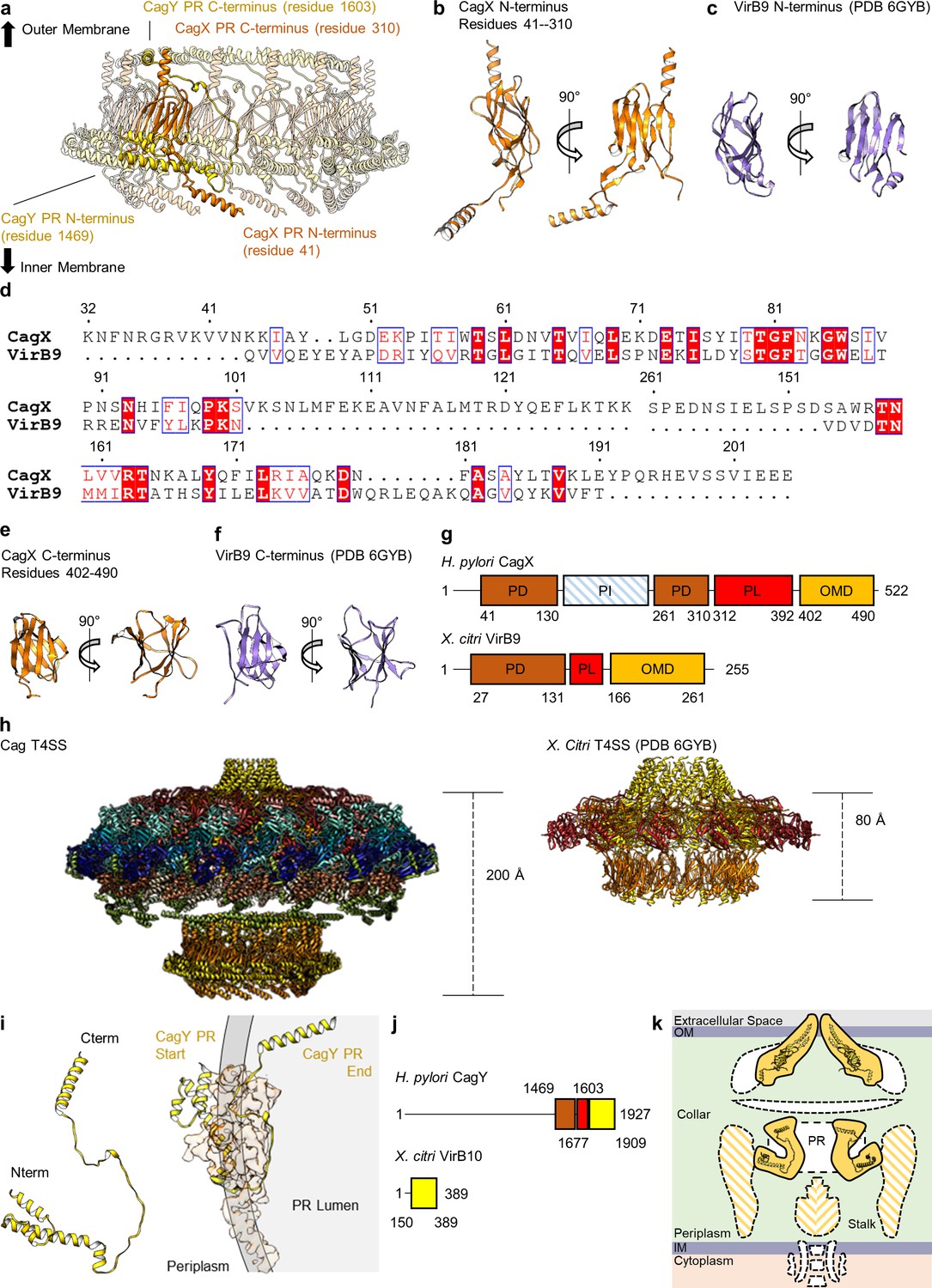
CagX and CagY comprise the PR.
(a) The PR is comprised of N-terminal portions of CagX and a fragment of CagY. Both proteins start from the inner membrane side of the PR, form small globular folds, and extend upward toward the outer membrane. A portion of CagY within the PR wraps around CagX, starting from the periplasm and winding into the lumen of the PR. (b) The N-terminal domain of CagX (residues 41–310) is similar to that of VirB9 (c) from X. citri in both structure and sequence (d). The C-terminal domain of CagX (e) is similar to that of the C-terminal domain of VirB9 from X. citri (f). (g) The periplasmic and outer membrane domains (PD and OMD, respectively) are similar in structurally characterized VirB9 homologs, though they are separated by a periplasmic linker (PL) that is variable in length. CagX contains an additional insertion (residues 102–153, periplasmic insertion or PI) that is unique when compared to other homologs. The structure corresponding to the PI was not observed within any of our cryo-EM reconstructions. (h) The spacing of the two CagX/VirB9 domains varies depending on the organism and appears to be highly dependent on the length of the periplasmic linker (CagX and VirB9 are shown in orange). (i) The segment of CagY within the PR (residues 1469–1603) adopts a highly elongated fold that consists of four α-helices (left). The periplasmic portion of CagY (as shown on the left) starts within the periplasm and wraps around the globular domain of CagX (shown in orange), eventually ending in the lumen of the PR (gray, right). (j) The periplasmic segment of CagY, which we call the periplasmic domain (PD, brown), is unique to CagY and is not present in other VirB10 homologs such as VirB10 from X. citri (yellow indicates a VirB10 like domain, and red represents the unstructured linker). (k) The N-terminus of CagY was not observed within any of these cryo-EM reconstructions. The N-terminal portion of CagY in the model that was constructed (about residue 1469) is positioned so that it might continue outward into the periplasmic space, possibly contributing to the structural feature known as the collar, as well as the stalk.
Figure 9
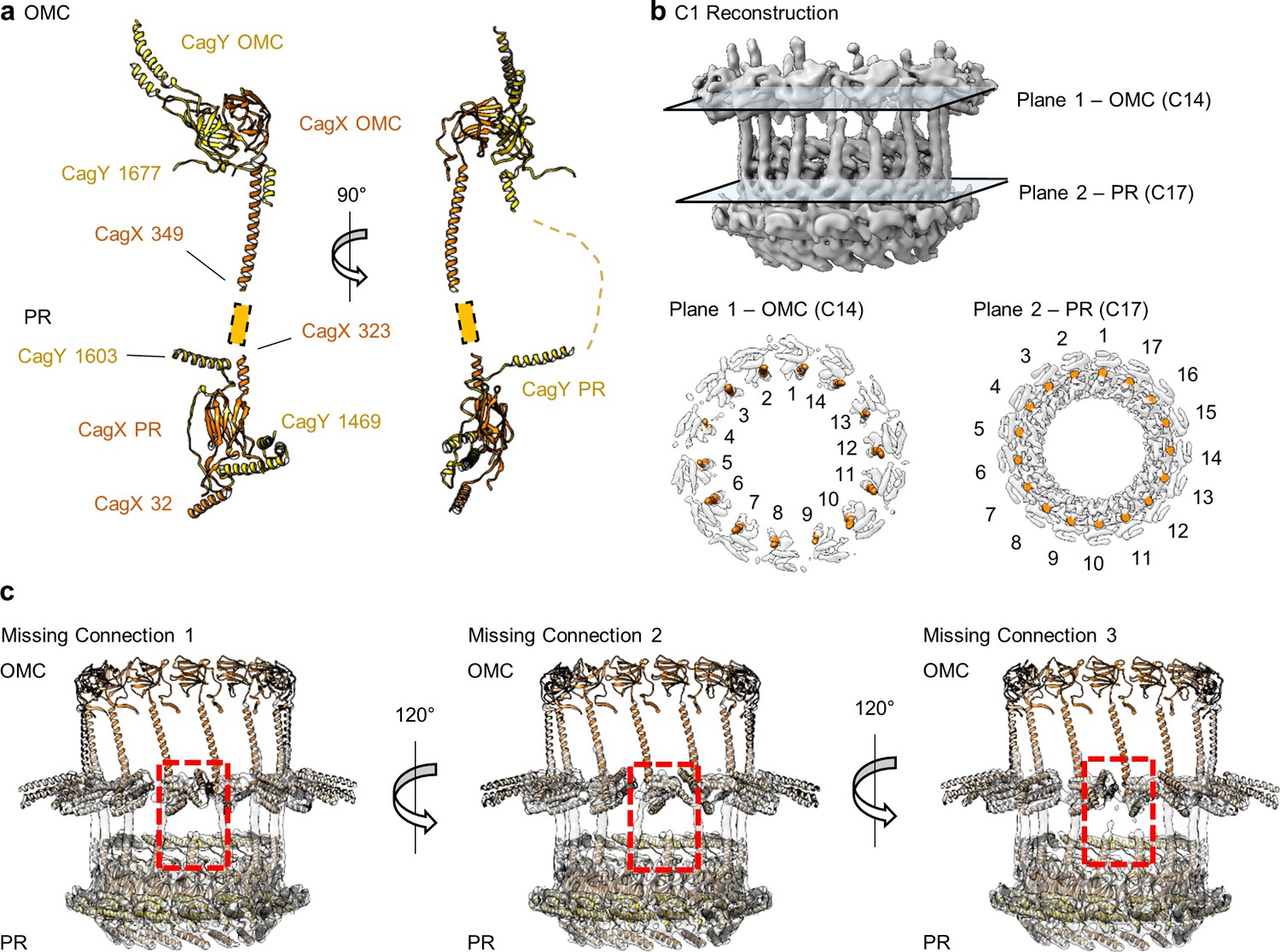
CagX and CagY span the symmetry mismatch between the OMC and PR.
(a) Models of CagX and CagY within the OMC and PR asymmetric units. (b) In the asymmetric reconstruction from a focused refinement of the interface between the OMC and PR of the WT map, we note the presence of helical density predicted to be a portion of CagX (top). We have modeled 14 copies of CagX into density within the OMC (bottom, left) and 17 copies of CagX into the PR (bottom, right). (c) Though we observe clear connections between 14 subunits of the OMC and 14 subunits of the PR, three copies of CagX in the PR do not show any obvious connection to the OMC.
Videos
Video 1
The Cag T4SS OMC.
Video 2
Differences between CagT-1 and CagT-2 in the Cag T4SS asymmetric unit.
Video 3
Arrangement of CagX and CagY within the PR of the Cag T4SS.
Video 4
Apparent Symmetry of CagX in the OMC and PR.
Tables
Key resources table
| Reagent type (species) or resource | Designation | Source or reference | Identifiers | Additional information |
|---|---|---|---|---|
| Strain, strain background (Helicobacter pylori 26695) | HA-CagF | PMID:26758182 | produces HA epitope-tagged CagF | |
| Strain, strain background (Helicobacter pylori 26695) | Δcag3; HA-CagF | PMID:26758182 | Δcag3 mutant, produces HA epitope-tagged CagF | |
| Software, algorithm | Leginon | PMID:15890530 | ||
| Software, algorithm | MotionCor2 | PMID:28250466 | ||
| Software, algorithm | CTFFind4 | PMID:26278980 | ||
| Software, algorithm | cryoSPARC | PMID:28165473 | ||
| Software, algorithm | RELION | PMID:27685097 PMID:30412051 | ||
| Software, algorithm | Coot | PMID:20383002 | ||
| Software, algorithm | UCSF Chimera | PMID:15264254 PMID:29340616 | ||
| Software, algorithm | PHENIX | PMID:29872004 | ||
| Software, algorithm | DALI server | PMID:31263867 |
Appendix 1—table 1
Cryo-EM data collection and processing.
| HpT4SS OMC WT | HpT4SS PC WT | HpT4SS OMC Δcag3 | HpT4SS PR Δcag3 | ||
|---|---|---|---|---|---|
| EMDB Accession Codes | EMD-22081 | EMD-20021 | EMD-22076 | EMD-22077 | |
| Data Collection and Processing | |||||
| Magnification | 18,000 | - | 29,000 | 29,000 | |
| Voltage (kV) | 300 | - | 300 | 300 | |
| Total Electron Dose (e-/Å2) | 59.0 | - | 59.7 | 59.7 | |
| Defocus Range (µm) | −2.5 ~ −3.5 | - | −1.5 ~ −3.5 | −1.5 ~ −3.5 | |
| Pixel Size (Å) | 1.64 | - | 1.0 | 1.0 | |
| Processing Software | CryoSPARC/Relion | - | CryoSPARC/Relion | CryoSPARC/Relion | |
| Symmetry | C14 | - | C14 | C17 | |
| Initial Particles (number) | 361,706 | - | 107,917 | 107,917 | |
| Final Particles (number) | 47,440 | - | 7337 | 10,477 | |
| Map Sharpening B Factor | −64.34 | - | −47.40 | −52.23 | |
| Map Resolution (Å) | 3.4 | - | 3.1 | 3.0 | |
| FSC Threshold | 0.143 | - | 0.143 | 0.143 | |
| Model Refinement and Validation | |||||
| Refinement | |||||
| Initial Model Used | 6OEF, 6OEE, 6ODI | 6X6L | 6OEF, 6OEE, 6ODI | 6OEF, 6OEE, 6ODI | |
| Model Resolution | |||||
| FSC (0.5) | 3.5 | 3.5 | 3.4 | 3.3 | |
| FSC (0.143) | 3.3 | 3.4 | 3.1 | 3.0 | |
| Model Composition (Residues) | 27,468 | 7602 | 5083 | ||
| Residues Modelled | |||||
| CagY | 1677–1820, 1851–1909 | 1469–1603 | 1677–1823, 1849–1910 | 1469–1603 | |
| CagX | 349–514 | 32–130, 261–325 | 361–515 | 32–130, 261–325 | |
| CagT-1 | 26–278 | - | 26–139, 165–175, 190–221, 286–307 | - | |
| CagT-2 | 29–139, 178–238, 254–273 | - | - | - | |
| Cag3-1 | 62–308 | - | - | - | |
| Cag3-2 | 104–193 | - | - | - | |
| Cag3-3 | 104–195 | - | - | - | |
| Cag3-4 | 74–79, 94–181 | - | - | - | |
| Cag3-5 | 78–181 | - | - | - | |
| CagM-1 | 187–366 | - | |||
| CagM-2 | 187–365 | - | - | ||
| Bond RMSD | |||||
| Bond Length (Å) | 0.011 | 0.006 | 0.011 | 0.007 | |
| Bond Angle (°) | 1.490 | 0.616 | 1.279 | 0.775 | |
| Validation | |||||
| Molprobity Score | 2.15 | 2.51 | 1.82 | 2.59 | |
| Clashscore | 9.64 | 13.41 | 8.21 | 11.66 | |
| Ramachandran (%) | |||||
| Favored | 94.0 | 95.9 | 94.5 | 96.4 | |
| Allowed | 6.0 | 4.1 | 5.5 | 3.6 | |
| Outliers | 0.0 | 0.0 | 0.0 | 0.0 | |
| B Factor | 127.48 | 95.94 | 75.84 | 76.90 | |
| PDB Accession Codes | 6X6S | 6X6J | 6X6K | 6X6L | |
Additional files
Download links
A two-part list of links to download the article, or parts of the article, in various formats.
Downloads (link to download the article as PDF)
Open citations (links to open the citations from this article in various online reference manager services)
Cite this article (links to download the citations from this article in formats compatible with various reference manager tools)
Cryo-EM reveals species-specific components within the Helicobacter pylori Cag type IV secretion system core complex
eLife 9:e59495.
https://doi.org/10.7554/eLife.59495


