Removing unwanted variation with CytofRUV to integrate multiple CyTOF datasets
- Bioinformatics Division, Walter and Eliza Hall Institute of Medical Research, Australia
- School of Mathematics and Statistics, The University of Melbourne, Australia
- The Walter and Eliza Hall Institute of Medical Research, Australia
- Department of Medical Biology, The University of Melbourne, Australia
Figures
Figure 1
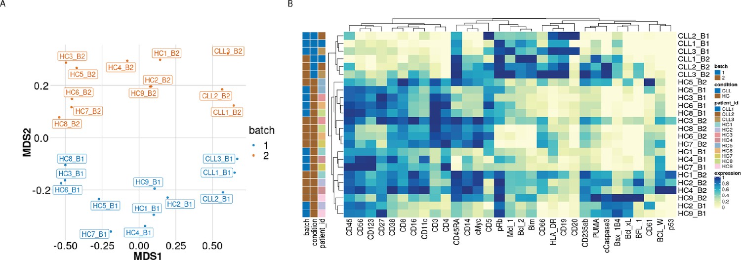
Visualisation of batch effects on the median protein expression across batches .
(A) Multi-dimensional scaling plot of the 24 samples computed using median protein expression. (B) Heatmap of the median protein expression of 19 lineage proteins and 12 functional proteins across all cells measured for each sample in the dataset.
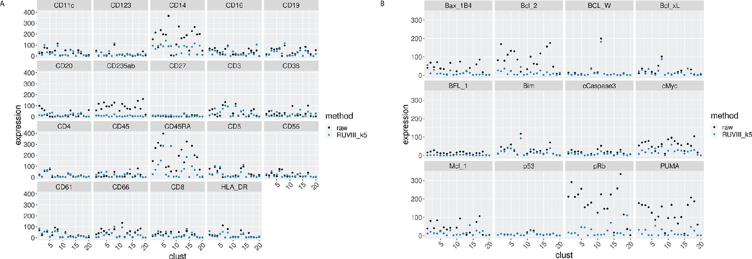
Figure 2 with 2 supplements
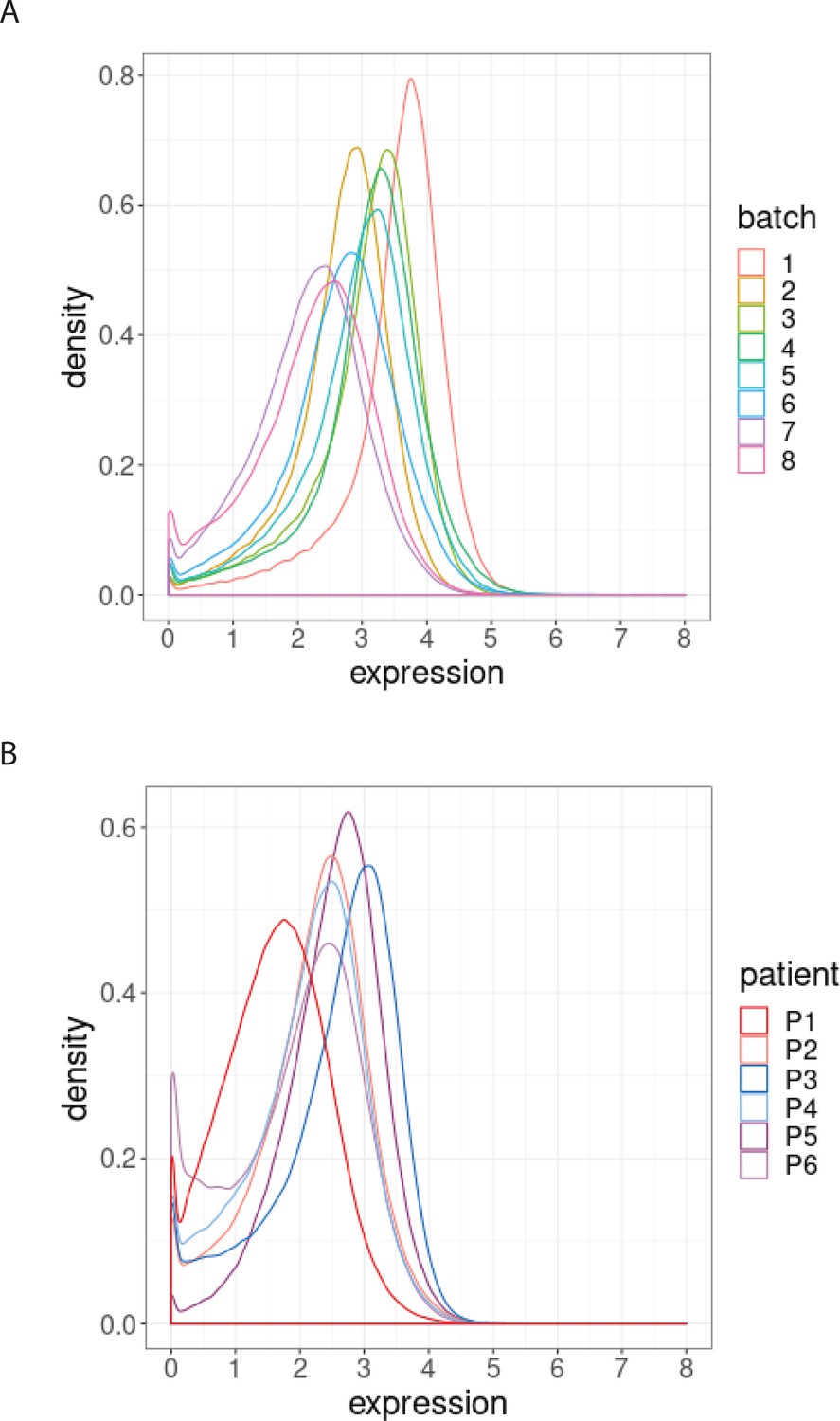
Distribution of BCL-2 expression.
(A) Distributions of BCL-2 expression in one sample from one treated CLL cancer patient, replicated across 8 CyTOF batches, coloured by batch. (B) Distributions of BCL-2 expression in one sample from each of 6 different CLL cancer patients at screening, processed in a single CyTOF batch, coloured by patient.
Figure 2—figure supplement 1
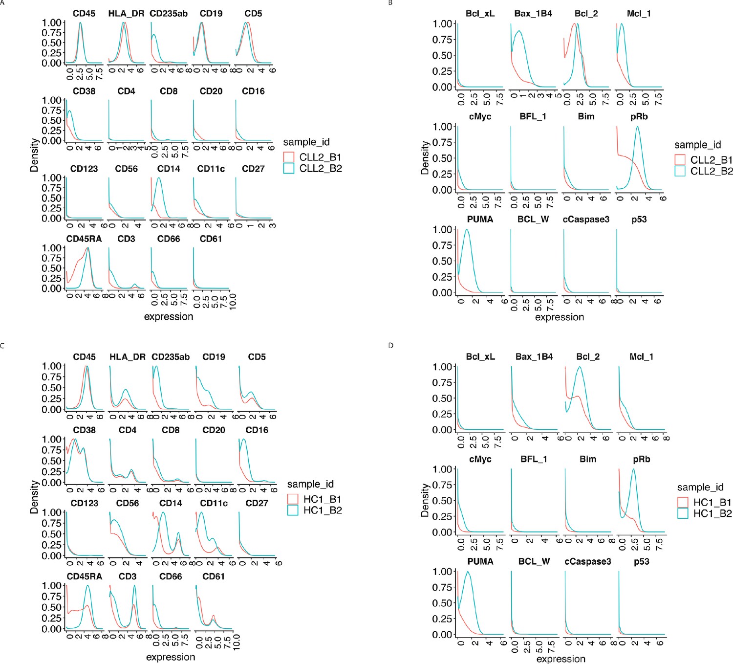
Protein distributions before normalisation for the samples CLL2 and HC1 across batch 1 and batch 2.
(A) Lineage protein expression distributions for the sample CLL2 across batches, before normalisation. (B) Same as (A) with functional proteins. (C) Lineage protein expression distributions for the sample HC1 across batches, before normalisation. (D) Same as (C) with functional proteins.
Figure 2—figure supplement 2
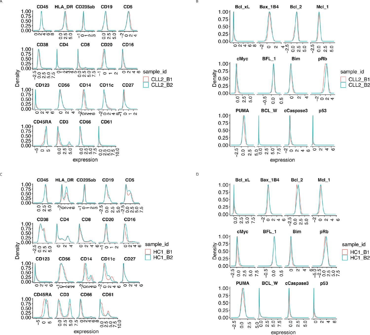
Protein distributions after CytofRUV normalisation with k = 5 for the samples CLL2 and HC1 across batch 1 and batch 2.
(A) Lineage protein expression distributions for the CLL2 sample across batches, after CytofRUV normalisation. (B) Same as (A) with functional proteins. (C) Lineage protein expression distributions for the sample HC1 across batches, after CytofRUV normalisation. (D) Same as (C) with functional proteins.
Figure 3 with 4 supplements
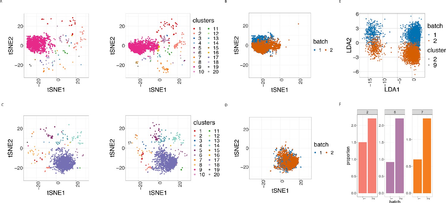
Cell clustering plots show batch effects in cells from the same cancer patient CLL1 sample replicated across 2 CyTOF runs.
(A) Cell clustering identification. t-SNE plot based on the arcsinh-transformed expression of the 19 lineage proteins in the cells. For display purposes, 2000 cells were randomly selected from each of the samples. Cells are coloured according to the 20 clusters obtained using FlowSOM clustering stratified by batch 1 (left) or 2 (right) of the corresponding replicated sample. (B) Same as in (A) selecting only cluster 9 cells but coloured by the batch 1 or 2 of the corresponding replicated sample. (C) Same as in (A) but after CytofRUV normalisation with k = 5. (D) Same as in (B) but after CytofRUV normalisation with k = 5. (E) Linear discriminant analysis applied to data on two cell types from the same sample replicated across two batches, with shape indicating cell type and colour indicating batch. (F) Cluster proportions. Barplot of the relative abundance (percentage) of the cells in clusters 2, 6 and 7 by batch.
Figure 3—figure supplement 1
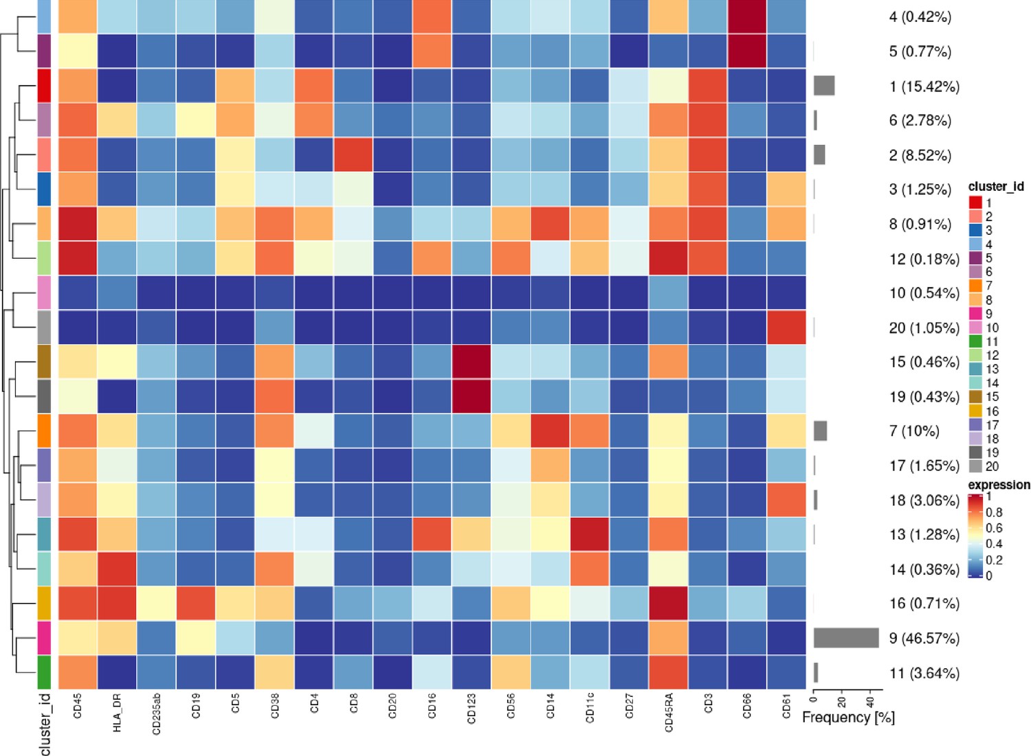
Heatmap of the median lineage protein expression across clusters with the associated cluster percentages measured for all cells and all samples in the first dataset of samples from 3 patients with CLL and 9 HC.
Figure 3—figure supplement 2
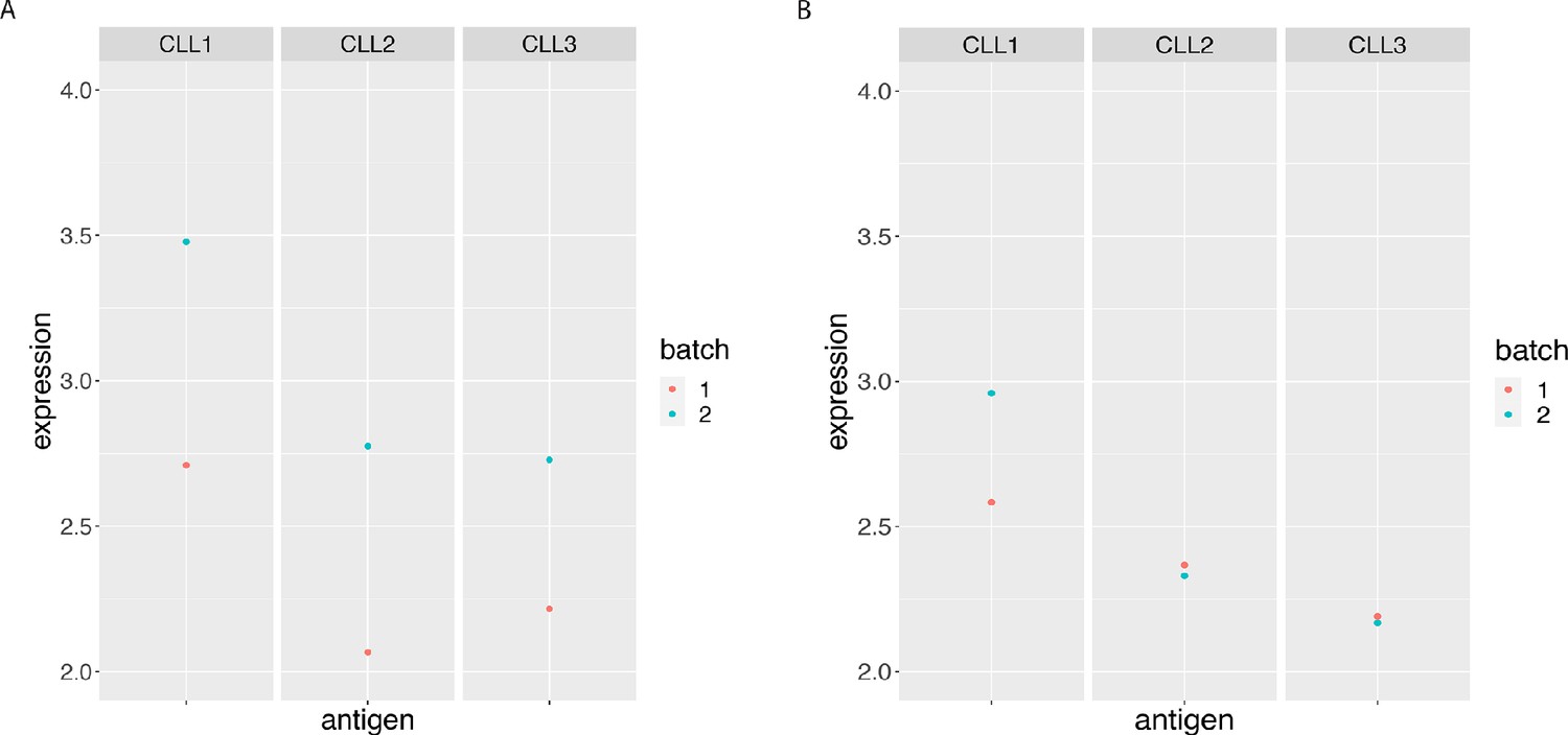
BCL-2 median expression in the main CLL cluster from the 3 CLL samples replicated across 2 CyTOF runs.
(A) Before and (B) After CytofRUV normalisation with k = 5.
Figure 3—figure supplement 3

Linear discriminant analysis plot to show batch effects in cells from the same cancer patient CLL1 sample replicated across batches after CytofRUV normalisation with k = 5.
Figure 3—figure supplement 4
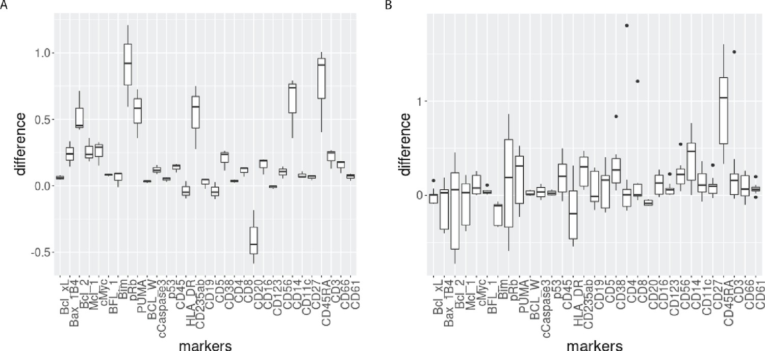
Boxplot of the differences of median protein expression differences across batches before and after CytofRUV normalisation (ΔΔ, see Materials and methods) with k=5 within the main prominent cell subpopulation.
(A) ΔΔ differences were computed on the 3 replicated CLL samples within the main CLL cluster. (B) ΔΔ differences were computed on the 9 replicated HC samples within the main HC cluster.
Figure 4
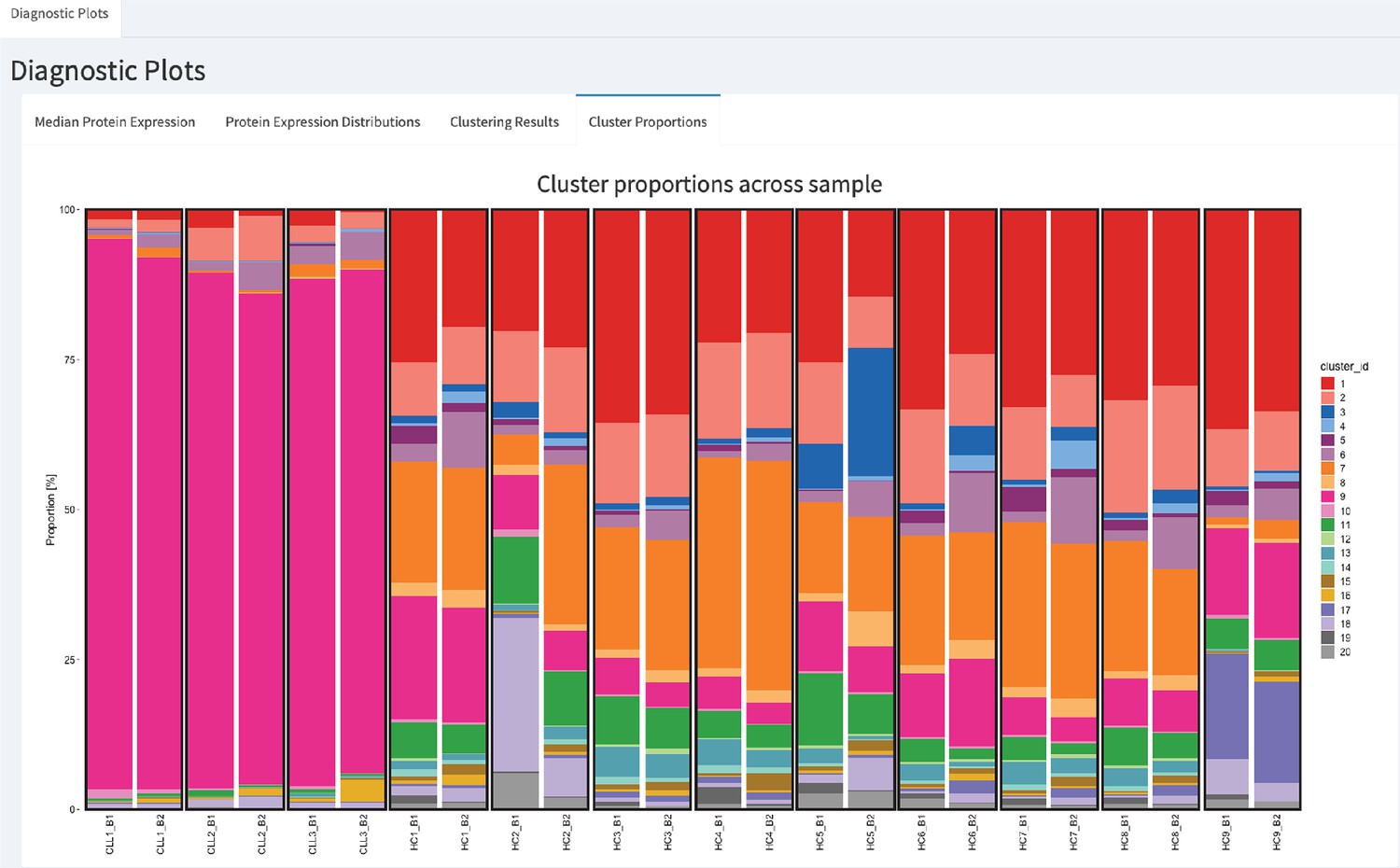
CytofRUV’s R-Shiny application for the identification of batch effects in cluster proportions across batches.
All diagnostic plots can be obtained by the user selecting an option at the top left corner by from: Median Protein Expression, Protein Expression Distributions, Clustering Results and Cluster Proportions. The selected option displays barplots of cluster proportions across samples before normalisation and by conditions CLL or HC on a subsample of the whole dataset. Vertical black boxes contain the same replicated sample across batches one and batch2.
Figure 5 with 1 supplement

Metrics to assess the effectiveness of the normalisation methods.
In all panels, the colour indicates either the raw data or the method used for normalisation. (A) Boxplots of the Earth Movers Distances (EMD) between paired protein expression distributions across batches for each CLL sample. (B) Hellinger distances between paired cluster proportions across batches for each CLL sample. (C) Mean Silhouette scores computed for all CLL samples on the cluster types (bio) on the x-axis and on batch (batch) on the y-axis. (D) Same as (A) for the HC samples. (E) Same as (B) for the HC samples. (F) Silhouette scores computed for all HC samples on the cluster types (bio) on the x-axis and on batch (batch) on the y-axis.
Figure 5—figure supplement 1
EMD for all the proteins by cluster, before and after CytofRUV normalisation of the CLL2 sample, k = 5.
(A) EMD for lineage proteins by cluster before (black) and after (blue) CytofRUV normalisation (blue). (B) Same as (A), with functional proteins.
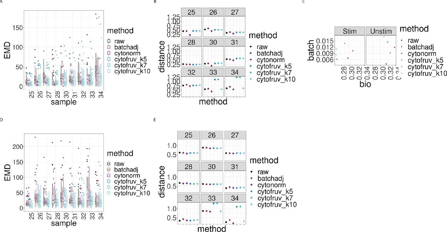
Figure 6 with 3 supplements
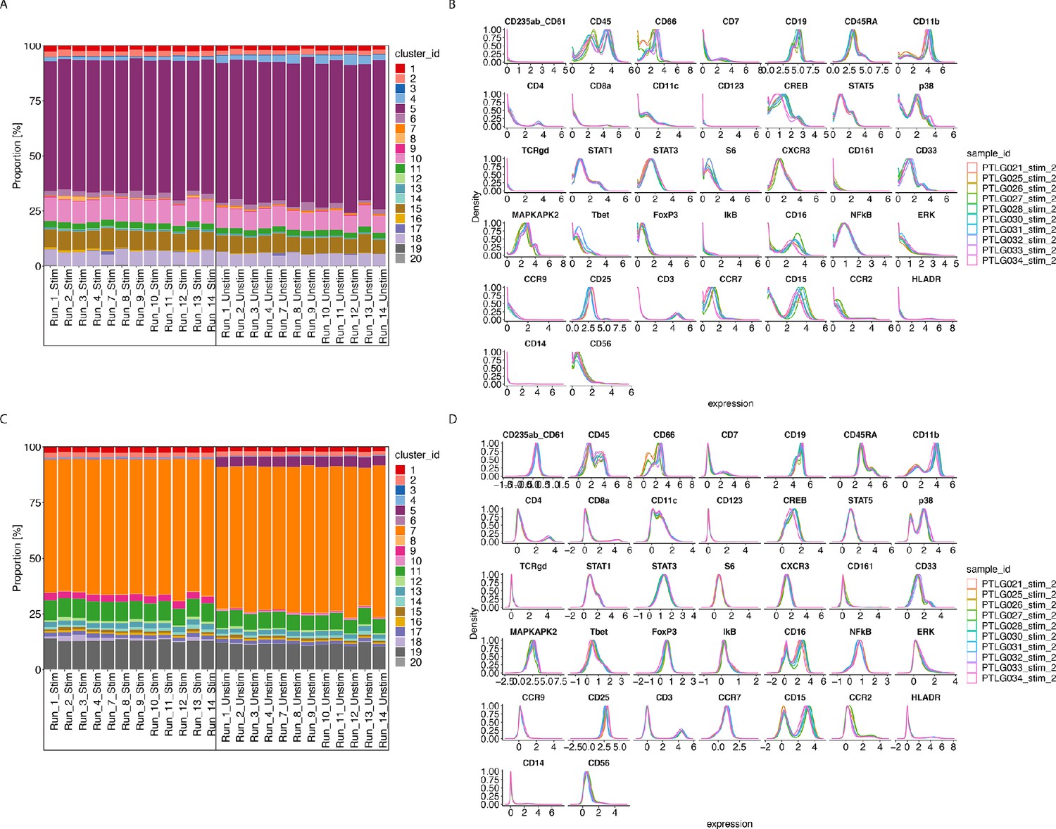
CytofRUV performance on two other datasets with multiple batches.
(A) Barplot of proportions of clusters across 28 samples from the BatchAdjust dataset (Schuyler et al., 2019) before normalisation, by samples and coloured by cluster. Vertical black boxes contain the same sample (Stimulated or Unstimulated) replicated across 14 batches. (B) Protein expression distribution from the CytoNorm dataset (Van Gassen et al., 2019) before normalisation of all cells from the stimulated samples across 10 batches and coloured by batch. (C) Same as (A) but after CytofRUV normalisation with k = 10. (D) Same as (B) but after CytofRUV normalisation with k = 5.
Figure 6—figure supplement 1
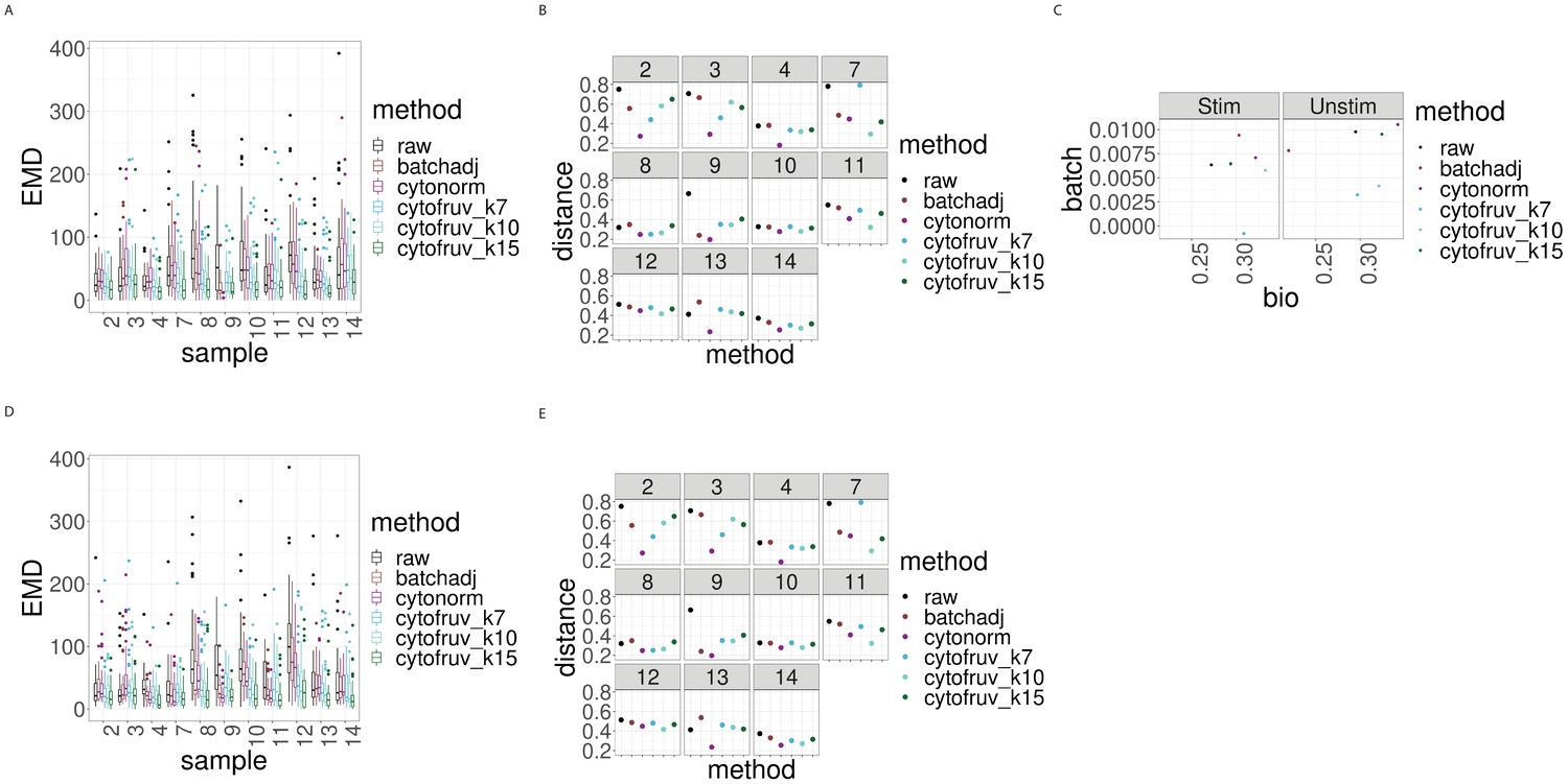
Metrics to assess the effectiveness of the normalisation methods on the BatchAdjust dataset.
In all panels, the colour indicates either the raw data or the method used for normalisation. (A) Boxplots of the Earth Movers Distance (EMD) between paired protein expression distributions for each batch’s stimulated sample compared to that in the first batch. (B) Hellinger distances between paired cell subpopulation proportions for each batch’s stimulated sample compared to that in the first batch. (C) Mean Silhouette scores computed for all stimulated and unstimulated samples with those for cell subpopulations (bio) on the x-axis and for batch (batch) on the y-axis. (D) Same as (A) for the unstimulated samples. (E) Same as (B) for the unstimulated samples.
Figure 6—figure supplement 2
Metrics to assess the effectiveness of the normalisation methods on samples two from the CytoNorm dataset using stimulated samples two as replicated reference samples.
In all panels, the colour indicates either the raw data or the method used for normalisation. (A) Boxplots of the Earth Movers Distance (EMD) between paired protein expression distributions for each batch’s stimulated sample across compared to that in the first batch. (B) Hellinger distances between paired cell subpopulation proportions for each batch’s stimulated sample compared to that in the first batch. (C) Mean Silhouette scores computed for all stimulated and unstimulated samples with those for cell subpopulations (bio) on the x-axis and for batch (batch) on the y-axis. (D) Same as (A) for the unstimulated samples. (E) Same as (B) for the unstimulated samples.
Figure 6—figure supplement 3
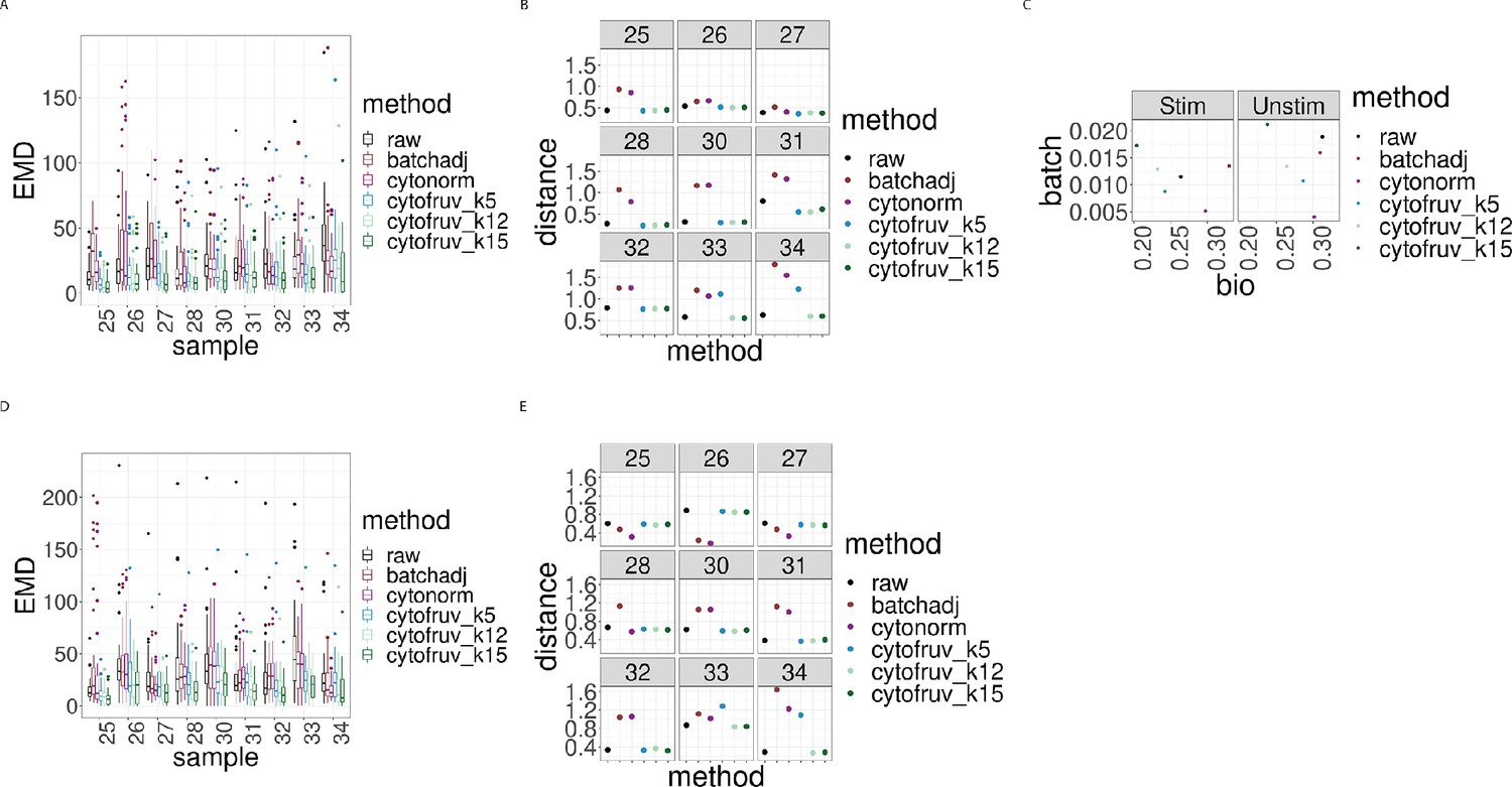
Metrics to assess the effectiveness of the normalisation methods on samples two from the CytoNorm dataset using both the stimulated and unstimulated samples one as replicated reference samples.
In all panels, the colour indicates either the raw data or the method used for normalisation. (A) Boxplots of the Earth Movers Distance (EMD) between paired protein expression distributions for each batch’s stimulated sample across compared to that in the first batch. (B) Hellinger distances between paired cell subpopulation proportions for each batch’s stimulated sample compared to that in the first batch. (C) Mean Silhouette scores computed for all stimulated and unstimulated samples with those for cell subpopulations (bio) on the x-axis and for batch (batch) on the y-axis. (D) Same as (A) for the unstimulated samples. (E) Same as (B) for the unstimulated samples.
Tables
Table 1
Samples descriptions.
The first column indicates the sample id, the second the patient condition, either healthy controls (HC) or chronic lymphocytic leukaemia (CLL), the third column indicates the patient id and the last indicates the batch number, 1 or 2.
| Sample Id | Condition | Patient Id | Batch |
|---|---|---|---|
| HC1_B1 | HC | VBDR996 | 1 |
| HC2_B1 | HC | VBDR1089 | 1 |
| HC3_B1 | HC | VBDR1090 | 1 |
| HC4_B1 | HC | VDBR1098 | 1 |
| HC5_B1 | HC | VDBR1108 | 1 |
| HC6_B1 | HC | VDBR1103 | 1 |
| HC7_B1 | HC | VDBR1105 | 1 |
| HC8_B1 | HC | VDBR1107 | 1 |
| HC9_B1 | HC | VBDR1111 | 1 |
| CLL1_B1 | CLL | DG33-01 | 1 |
| CLL2_B1 | CLL | DG23-01 | 1 |
| CLL3_B1 | CLL | DG27-01 | 1 |
| HC1_B2 | HC | VBDR996 | 2 |
| HC2_B2 | HC | VBDR1089 | 2 |
| HC3_B2 | HC | VBDR1090 | 2 |
| HC4_B2 | HC | VDBR1098 | 2 |
| HC5_B2 | HC | VDBR1108 | 2 |
| HC6_B2 | HC | VDBR1103 | 2 |
| HC7_B2 | HC | VDBR1105 | 2 |
| HC8_B2 | HC | VDBR1107 | 2 |
| HC9_B2 | HC | VBDR1111 | 2 |
| CLL1_B2 | CLL | DG33-01 | 2 |
| CLL2_B2 | CLL | DG23-01 | 2 |
| CLL3_B2 | CLL | DG27-01 | 2 |
Table 2
Lineage surface proteins selected.
The first column indicates the transition element isotope (mass number, element name), the second column indicates the antigen selected, and the last two columns indicate the clone name and vendor.
| Metal | Lineage (surface) protein antibody | Clone | Vendor | |
|---|---|---|---|---|
| 1 | 89 Y | CD45 | HI30 | BioLegend |
| 2 | 115 In | HLA-DR | L243 | BioLegend |
| 3 | 140 Ce | CD27 | M-T271 | BioLegend |
| 4 | 141 Pr | CD235a/b | HIR2 | BioLegend |
| 5 | 142 Nd | CD19 | HIB19 | BioLegend |
| 6 | 143 Nd | CD5 | UCHT2 | BioLegend |
| 7 | 144 Nd | CD38 | HIT2 | BioLegend |
| 8 | 145 Nd | CD4 | RPA-T4 | BioLegend |
| 9 | 146 Nd | CD8 | RPA-T8 | BioLegend |
| 10 | 147 Sm | CD20 | H1 | BD |
| 11 | 148 Nd | CD16 | 3G8 | BioLegend |
| 12 | 151 Eu | CD123 | 6H6 | BioLegend |
| 13 | 155 Gd | CD56 | B159 | BioLegend |
| 14 | 156 Gd | CD14 | HCD56 | BioLegend |
| 15 | 159 Tb | CD11c | Bu15 | BioLegend |
| 16 | 169 Tm | CD45RA | HI100 | BioLegend |
| 17 | 170 Er | CD3 | UCHT1 | BioLegend |
| 18 | 171 Yb | CD66 | CD66a-B1.1 | DVS |
| 19 | 209 Bi | CD61 | VI-PL2 | DVS |
Table 3
Set of intracellular functional proteins selected.
The first column transition element isotope (mass number, element name), the second column indicates the antigen selected, and the last two columns indicate the clone name and vendor.
| Metal | Functional (intracellular) protein antibody | Clone | Vendor | |
|---|---|---|---|---|
| 1 | 140 Ce | BAK | 7D10 | WEHI |
| 2 | 153 Eu | Bcl-xL | E18 | Abcam |
| 3 | 154 Sm | Bax | 1B4 | WEHI |
| 4 | 157 Gd | Bcl-2 | 100 | WEHI |
| 5 | 160 Gd | Mcl-1 | Y37 | Abcam |
| 6 | 161 Dy | cMyc | D84C12 | CST |
| 7 | 163 Dy | BFL-1 | SP435 | Abcam |
| 8 | 165 Ho | Bim | 3C5 | WEHI |
| 9 | 166 Er | pRb [S807/811] | J112-906 | BD |
| 10 | 172 Yb | BCLW | 16H12 | WEHI |
| 11 | 173 Yb | cCaspase3 | C92-605 | BD |
| 12 | 174 Yb | p53 | 7F5 | CST |
Additional files
-
Supplementary file 1
Scripts to generate the CytofRUV figures from the dataset FR-FCM-Z2L2.
CytofRUV_preprocessing_dataset.R is the script that was used to generate the preprocessing on the dataset: data concatenation, normalisation and debarcoding are done using the R Catalyst package merging the two batches (RUV_1B and RUV3B) when applying the Finck normalisation. CytofRUV_Figures.R was used to generate the figures described in this manuscript and uses the CytofRUV R package with the Metadata.xlsx and Panel.xlsx files. The package is available at: www.github.com/mtrussart/CytofRUV. Installation and R code usage instructions for both the R package and the R-Shiny application can be found on the GitHub page.
- https://cdn.elifesciences.org/articles/59630/elife-59630-supp1-v3.zip
-
Transparent reporting form
- https://cdn.elifesciences.org/articles/59630/elife-59630-transrepform-v3.docx
Download links
A two-part list of links to download the article, or parts of the article, in various formats.
Downloads (link to download the article as PDF)
Open citations (links to open the citations from this article in various online reference manager services)
Cite this article (links to download the citations from this article in formats compatible with various reference manager tools)
Removing unwanted variation with CytofRUV to integrate multiple CyTOF datasets
eLife 9:e59630.
https://doi.org/10.7554/eLife.59630


