Learning excitatory-inhibitory neuronal assemblies in recurrent networks
- Bernstein Center for Computational Neuroscience Berlin, Germany
- Department for Electrical Engineering and Computer Science, Technische Universität Berlin, Germany
Figures
Figure 1 with 5 supplements
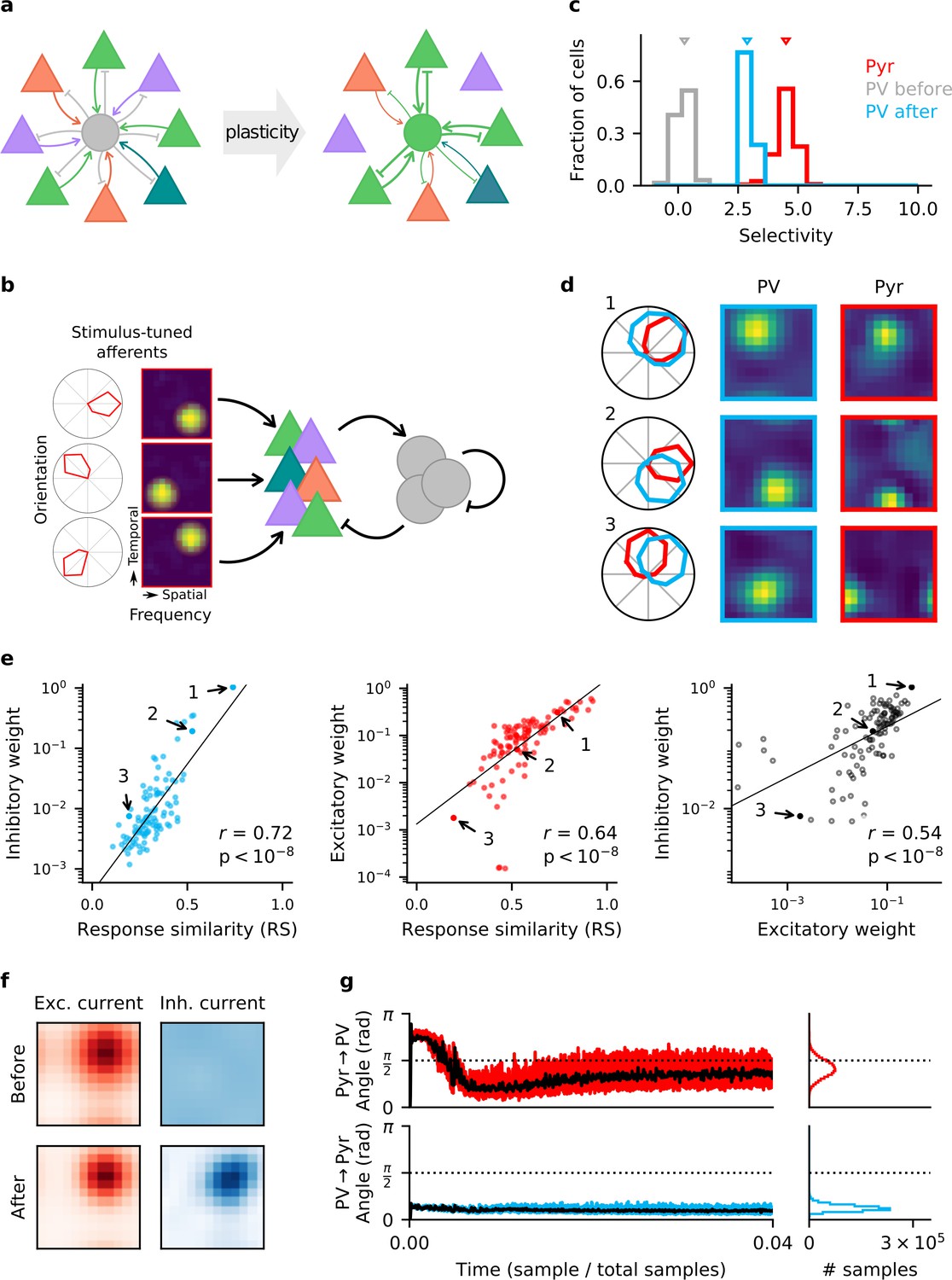
Homeostatic plasticity in input and output synapses of interneurons drives the formation of excitatory-inhibitory (E/I) assemblies.
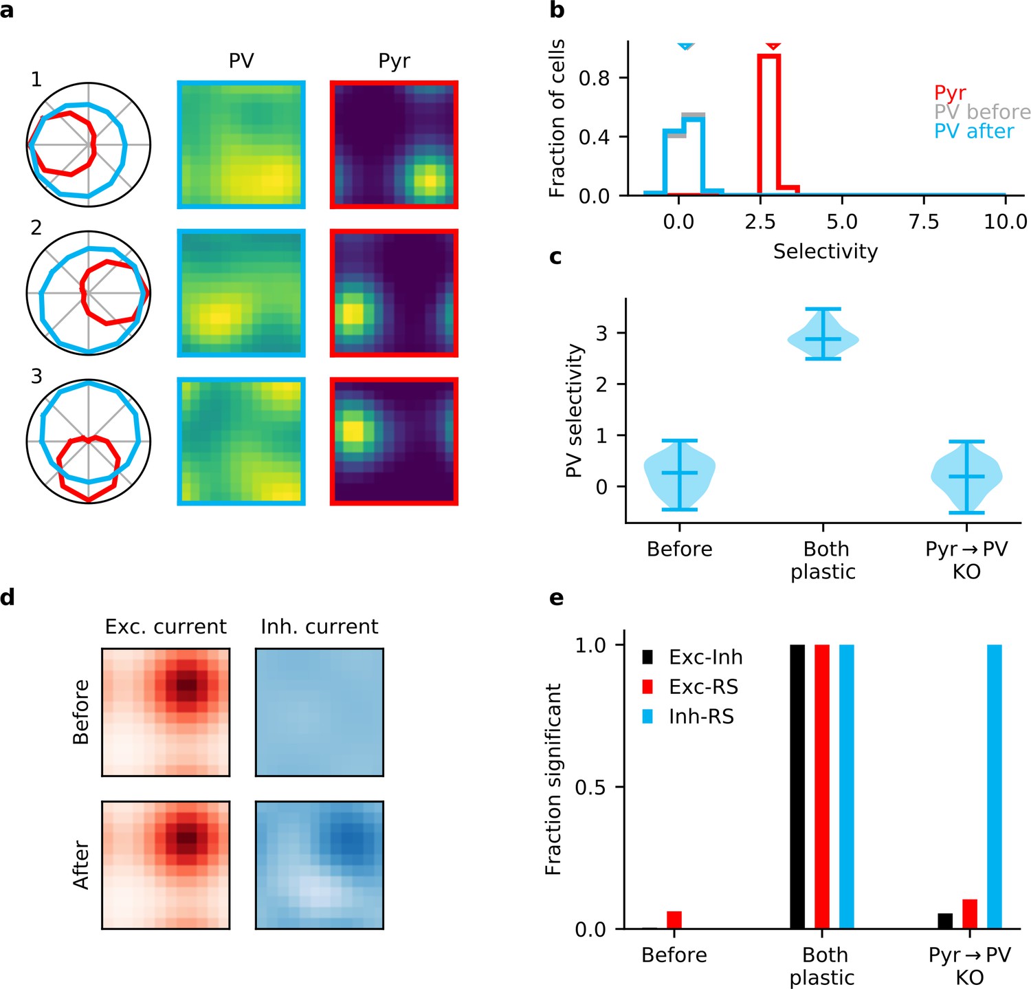
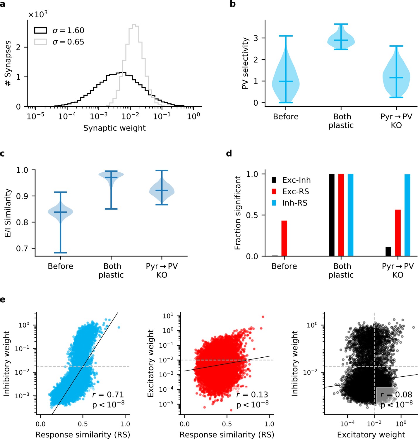
(a) Emergence of E/I assemblies comprised of pyramidal (Pyr) neurons (triangles) and parvalbumin-expressing (PV) interneurons (circles) in circuits without feature topography. (b) Network architecture and stimulus tuning of external inputs to Pyr cells. (c) Stimulus selectivity of Pyr neurons and PV interneurons (before and after learning). Arrows indicate the median. (d) Example responses of reciprocally connected Pyr cells and PV interneurons. Examples chosen for large, intermediate, and low response similarity (RS). Numbers correspond to points marked in (e). (e) Relationship of synaptic efficacies of output (left) and input connections (centre) of PV interneurons with RS. Relationship of input and output efficacies (right). Black lines are obtained via linear regression. Reported r and associated p-value are Pearson’s correlation. (f) Stimulus tuning of excitatory and inhibitory currents onto an example Pyr cell, before and after learning. For simplicity, currents are shown for spatial and temporal frequency only, averaged across all orientations. (g) Angle between the weight update and the gradient rule while following the local approximation for input (top) and output (bottom) connections of PV interneurons. Time course for first 4% of simulation (left) and final distribution (right) shown. Black lines are low-pass filtered time courses.
Figure 1—figure supplement 1
Synaptic plasticity and convergence.
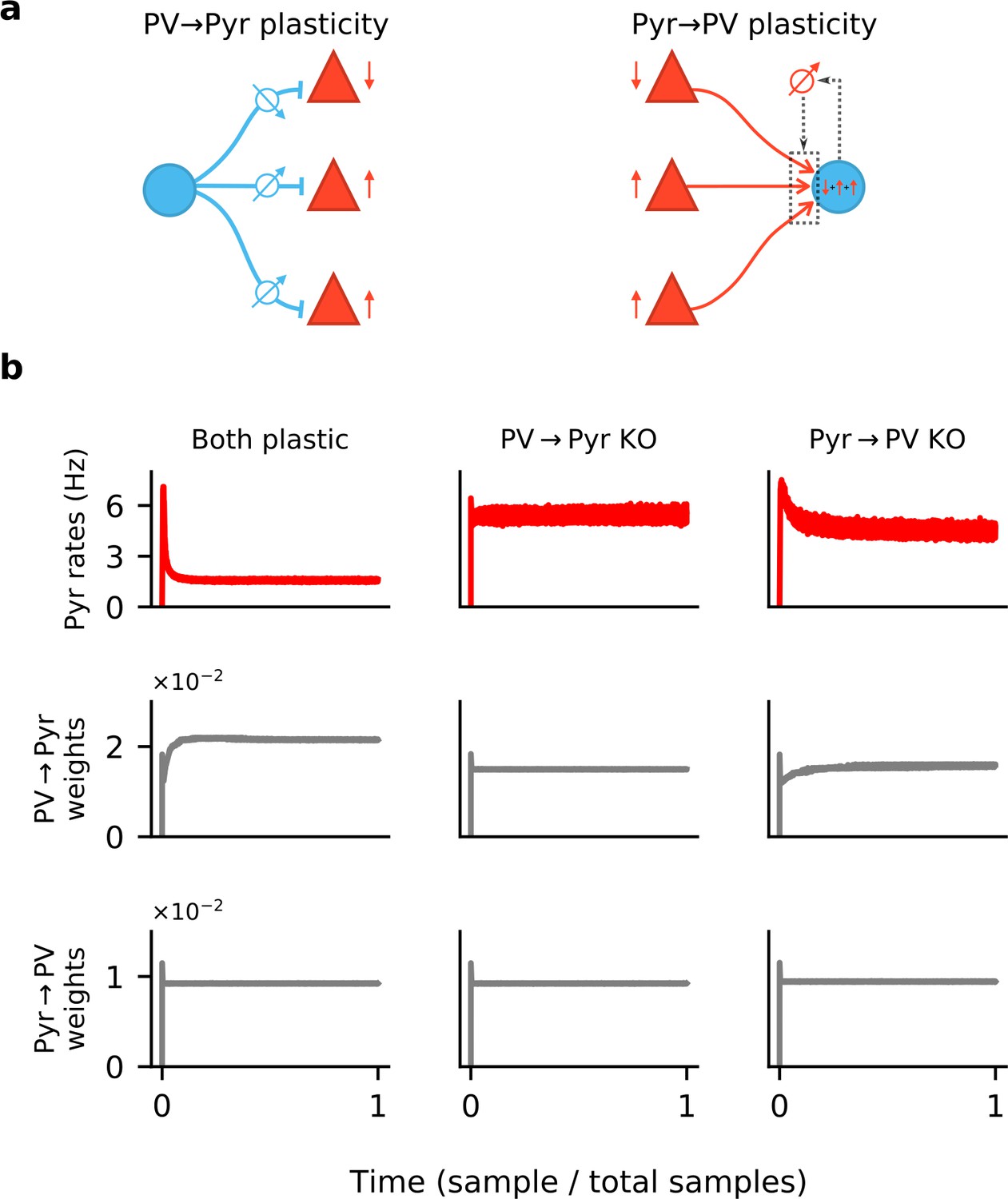
(a) Schematics of PV → Pyr plasticity (left) and Pyr → PV plasticity (right). PV → Pyr plasticity follows a simple logic: A given inhibitory synapse is potentiated if the postsynaptic Pyr neuron fires above target and is depressed if below. The Pyr → PV plasticity compares the excitatory input current received by the postsynaptic PV neuron to a target value, and adjusts the incoming synapses in proportion to this error and to presynaptic activity. (b) Time plots of the Pyr population firing rate (top), mean of all PV → Pyr synaptic weights (middle) and Pyr → PV weights (bottom). Columns correspond to simulations in which both PV → Pyr and Pyr → PV plasticity are present (left), only Pyr → PV is present (middle), and only PV → Pyr is present (right).
Figure 1—figure supplement 2
Gradient rules also require plasticity of both input and output synapses of parvalbumin-expressing (PV) interneurons.
(a) In a network learning with the derived gradient rules of Equation 15, significant correlations are reliably detected between response similarity (RS) and excitatory weights (red bars), RS and inhibitory weights (blue bars), and excitatory and inhibitory weights for reciprocally connected pyramidal (Pyr)-PV cell pairs (black bars) only if both synapse types are plastic. (b) Interneurons fail to develop stimulus selectivity if their input weights do not change according to the gradient rule of Equation 15a. (c) Synaptic currents onto Pyr neurons only develop reliable, strong excitatory-inhibitory (E/I) co-tuning if both input and output synapses are updated using the gradient rules. Currents are averaged across all Pyr neurons after centring according to the neuron’s preferred stimulus. The bottom row is a slice through the difference (third row) of the average excitatory (first row) and inhibitory currents (second row). (d) Violin plot of the distribution of E/I synaptic current similarity values for all Pyr neurons in the network (see Materials and methods).
Figure 1—figure supplement 3
Synaptic currents onto pyramidal (Pyr) neurons.
(a) Excitatory (red) and inhibitory (blue) synaptic currents onto a random selection of Pyr neurons, as a function of temporal and spatial stimulus frequency (averaged over all orientations), when both incoming and outgoing parvalbumin-expressing (PV) synapses are plastic. (b) The network-averaged excitatory (first row) and inhibitory (second row) synaptic currents onto Pyr neurons, both centred according to the peak excitatory current before averaging. After averaging, their difference is taken (third row) and a slice is plotted (bottom row). When both plasticities are present, currents are well balanced across stimuli with a modest excitatory bias for preferred stimuli. (c) Quality of excitatory-inhibitory (E-I) current co-tuning for every Pyr in the network quantified by the distribution of their cosine similarities. Only when both plasticities are present, do most Pyr neurons receive well co-tuned E-I synaptic currents.
Figure 1—figure supplement 4
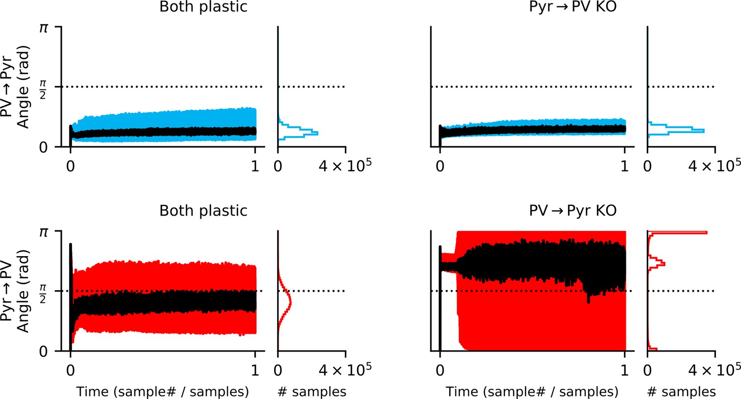
Both input and output synapses must be plastic for feedback alignment to occur.
In a network with both local rules (left column), the update to Pyr → PV synapses rapidly aligns to the gradient (i.e. when the angle between the approximate update and the gradient is below ; bottom left). While updates to the Pyr → PV weights occasionally point away from the gradient, 79% of samples are below . For the knock-out (KO) experiments (right column), output plasticity closely follows the PV → Pyr gradient even if input plasticity is absent (upper right). In contrast, if output (PV → Pyr) plasticity is absent, the approximate Pyr → PV rule does not follow the gradient (lower right).
Figure 1—figure supplement 5
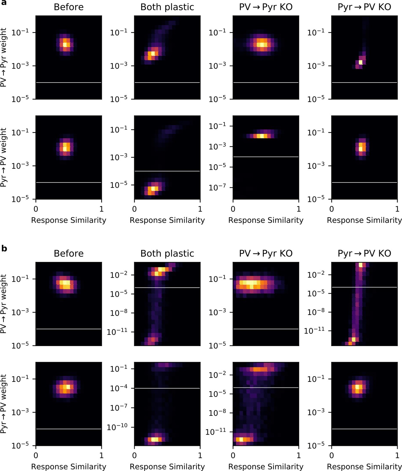
Some networks contain experimentally undetectable weights.
(a) Plots of 2D histograms for PV → Pyr (top) and Pyr → PV (bottom) weight versus response similarity (RS), in different networks trained with the local plasticity rules (columns). White lines indicate the threshold of experimental detectability. Any weight < 10-4 is not included when computing Pearson’s correlation between RS and synaptic weight, or weight-weight correlations. (b) Same plots as (a), but for networks trained with the gradient rules.
Figure 2

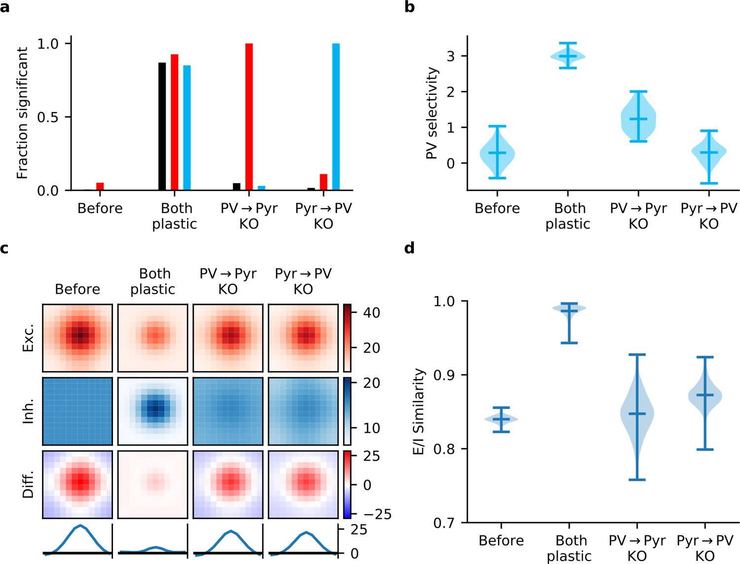
Knock-out (KO) of plasticity in parvalbumin-expressing (PV) interneuron output connections prevents inhibitory co-tuning.
(a) Example responses of reciprocally connected pyramidal (Pyr) cells and PV interneurons. Numbers correspond to points marked in (d). (b) Stimulus selectivity of Pyr cells and PV interneurons (before and after learning; Mann-Whitney U test, ). Arrows indicate median. (c) Stimulus tuning of excitatory and inhibitory input currents in a Pyr cell before and after learning. For simplicity, currents are shown for spatial and temporal frequency only, averaged across all orientations. (d) Relationship of output (left) and input (centre) synaptic efficacies of PV interneurons with response similarity. Relationship of input and output efficacies (right). Plotted lines are obtained via linear regression. Reported r and associated p-value are the Pearson’s correlation. (e) Distribution of Pearson’s correlation coefficients for multiple samples as shown in (d). Dashed line marks threshold of high significance (). (f) Fraction of samples with highly significant positive correlation before plasticity, after plasticity in both input and output connections, and for KO of plasticity in PV output connections (based on 10,000 random samples of 100 synaptic connections).
Figure 3 with 2 supplements
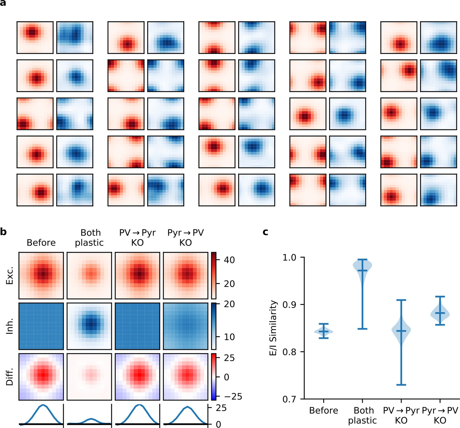
Plasticity of parvalbumin-expressing (PV) interneuron input connections is required for inhibitory stimulus selectivity and current co-tuning.
(a) Example responses of reciprocally connected pyramidal (Pyr) cells and PV interneurons. (b) Stimulus selectivity of Pyr cells and PV interneurons (before and after learning). Arrows indicate median. (c) Violin plots of inhibitory stimulus selectivity before plasticity, after learning with plasticity in both input and output connections of PV interneurons and for knock-out (KO) of plasticity in PV input connections. (d) Stimulus tuning of excitatory and inhibitory currents in a Pyr cell before and after learning. Dimensions correspond to spatial and temporal frequency of the stimuli averaged across all orientations. (e) Fraction of samples with highly significant () positive correlation before plasticity, after plasticity in both input and output connections, and for KO of plasticity in PV input connections (based on 10,000 random samples of 100 synaptic connections).
Figure 3—figure supplement 1
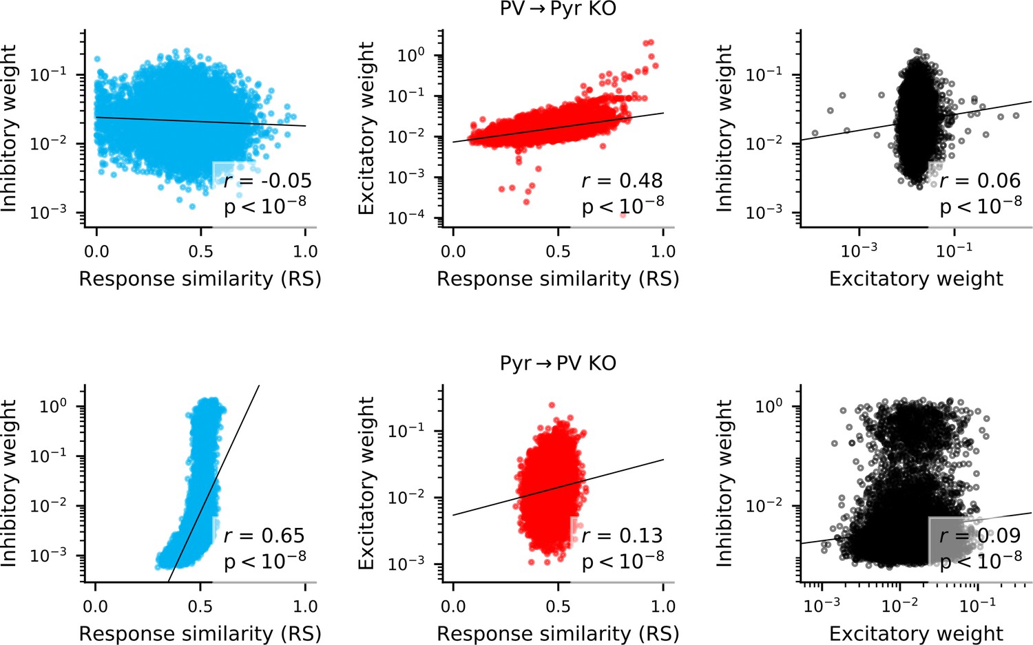
Correlation between weights and response similarity.
Scatter plots containing every synapse in networks without PV → Pyr plasticity (top), or without Pyr → PV plasticity (bottom). Pearson’s correlation is always highly significant, though sometimes weak.
Figure 3—figure supplement 2
Long-tailed Pyr → PV weight distribution does not reproduce experimentally observed correlations.
To ensure that the results of Figure 3 were not simply a consequence of our chosen Pyr → PV weight distribution (), we repeat those simulations with weights drawn from a log-normal distribution with a longer tail (). (a) The default and longer-tailed distributions of Pyr → PV weights. (b) PV neurons exhibit greater stimulus selectivity than in Figure 3, when Pyr→ PV plasticity is knocked out. (c) Excitatory currents are more precisely balanced by inhibition (compare with Figure 3). (d) When repeatedly sampling 100 synapses, the strength of inhibitory synapses that connect Pyr and PV cell pairs are always significantly correlated () with response similarity (RS). Excitatory synapses between cell pairs are only correlated with RS in about half of the samples. For reciprocally connected cell pairs, the strength of excitatory weights is rarely correlated with the inhibitory weights. (e) Similar to Figure 3—figure supplement 1 (bottom), when all synapses for the Pyr → PV KO network are considered, Exc-RS and Exc-Inh correlations are weak but highly significant. Dashed lines indicate the threshold below which synapses are considered experimentally undetectable and discarded for the analysis in (d).
Figure 4 with 1 supplement

Single-neuron perturbations suppress responses of similarly tuned neurons.
(a) Perturbation of a single pyramidal (Pyr) neuron. Responses of other Pyr neurons are recorded for different stimuli, both with and without perturbation. (b) Perturbation-induced change in activity ( Act.) of a subset of Pyr cells, for a random subset of stimuli (with neuron 1 being perturbed). (c) Influence of perturbing a Pyr neuron on the other Pyr neurons, averaged across all stimuli, for a subset of Pyr neurons. (d) Dependence of influence among Pyr neurons on their receptive field correlation (Pearson’s r), across all neurons in the network (see 'Materials and methods'). Dotted lines indicate plasticity knock-out (KO) experiments; see Figure 4—figure supplement 1b for details. Error bars correspond to the standard error of the sample mean, but are not visible due to their small values. (e) Total strength of output synapses from a Pyr neuron predicts the average effect perturbing it has on other neurons. Dashed line is the result of a linear regression, while r and its associated p-value correspond to the Pearson’s correlation.
Figure 4—figure supplement 1
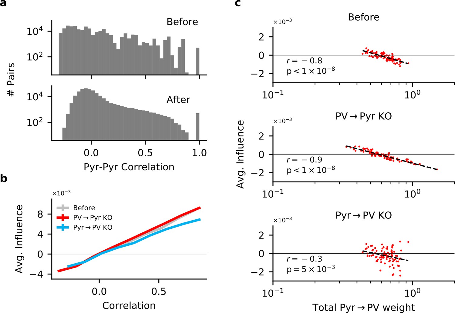
Input and output plasticity together change correlations between pyramidal (Pyr) neurons, while plasticity knock-out (KO) eliminates feature competition.
(a) Receptive field correlations (Pearson’s) between Pyr neurons, before (top) and after (bottom) learning with both PV → Pyr and Pyr → PV synaptic plasticity. (b) The effect of perturbing a Pyr neuron on the response of other Pyr neurons (to random stimuli) as a function of their receptive field correlation (see 'Materials and methods'). On their own, both Pyr → PV and PV → Pyr plasticity have little effect on the feature amplification observed prior to learning. (c) Despite the absence of feature competition on average in the KO networks, the total strength of Pyr → PV synapses from a given Pyr neuron is still predictive of its influence on the rest of the network: The stronger its total weight, the more likely a Pyr is to suppressing the response of other Pyr neurons.
Tables
Table 1
Model parameters.
| 512 | 64 | Number of exc. and inh. neurons. | ||
|---|---|---|---|---|
| 50 ms | 25 ms | Rate dynamics time constants | ||
| 1 ms | Numerical integration time step | |||
| 0.6 | 0.6 | Connection probability to exc. and inh. neurons | ||
| 2 | 5 | Total of exc. weights onto neuron i: | ||
| 1 | 1 | Total of inh. weights onto neuron i: | ||
| 0.65 | 0.65 | Std. deviation of the logarithm of the weights | ||
| Experimental detection threshold for synapses | ||||
| 5 Hz | 50 Hz | Background and maximum stimulus-specific input | ||
| 500 | Number of stimuli and trials | |||
| 1 | Range of stimuli and Pyr RF von Mises width | |||
| 10 Hz | Change of input for perturbation experiments | |||
| Learning rates (approximate and gradient rules) | ||||
| 0.1 | 0.1 | Weight decay rates | ||
| 1 Hz | Homeostatic plasticity target | |||
| 0.9 | 0.999 | Adam parameters for gradient rules | ||
Additional files
Download links
A two-part list of links to download the article, or parts of the article, in various formats.
Downloads (link to download the article as PDF)
Open citations (links to open the citations from this article in various online reference manager services)
Cite this article (links to download the citations from this article in formats compatible with various reference manager tools)
Learning excitatory-inhibitory neuronal assemblies in recurrent networks
eLife 10:e59715.
https://doi.org/10.7554/eLife.59715


