An approach for long-term, multi-probe Neuropixels recordings in unrestrained rats
- Princeton Neuroscience Institute, United States
- Howard Hughes Medical Institute, Princeton University, United States
Figures
Figure 1
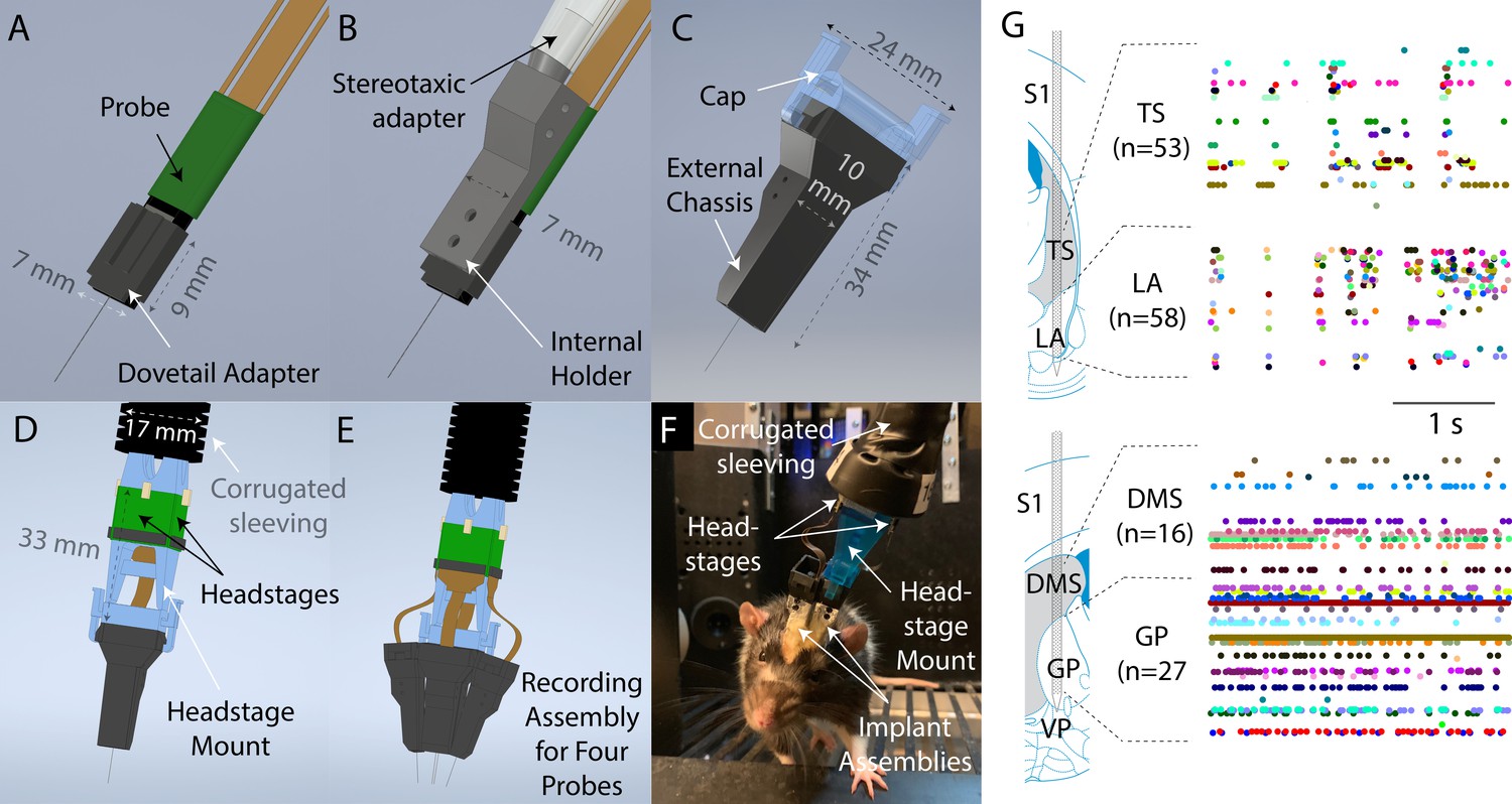
Design overview.
(A) To prepare a probe for implantation, it is first mounted to a dovetail adapter. (B) The dovetail adapter mates with an internal holder through a dovetail joint. The internal holder can be manipulated with a commercially available stereotaxic holder. (C) The entire apparatus is then enclosed with, and screwed onto, an external chassis. During the surgery, the external chassis, but not the internal holder, is fixed to the skull surface. Therefore, the internal holder and probe could be fully removed at the end of the experiment simply by unscrewing them from the external chassis. The external chassis contains a mechanism to allow a cap to be latched on top to protect the probe when recording is not taking place. (D) Using the same latching mechanism, a headstage mount can be connected to the assembly for recording instead of the cap shown in (C). The headstage mount is fixed to a corrugated plastic sleeving, which protects the cables from small bending radii, and contains space for up to four headstages. (E) Schematic illustration of the full recording system for four probes simultaneously implanted. (F) A photograph of a rat in a behavioral rig with two probes implanted and with a headstage mount connected for recording. (G) Simultaneous recordings from two Neuropixels probes in a moving rat. Top: recording from tail of striatum (TS) and lateral amygdala (LA). Bottom: recording from dorsomedial striatum (DMS) and globus pallidus (GP). Images and schematic are adapted from Paxinos and Watson, 2006. Colored dots indicate spike times.
Figure 2
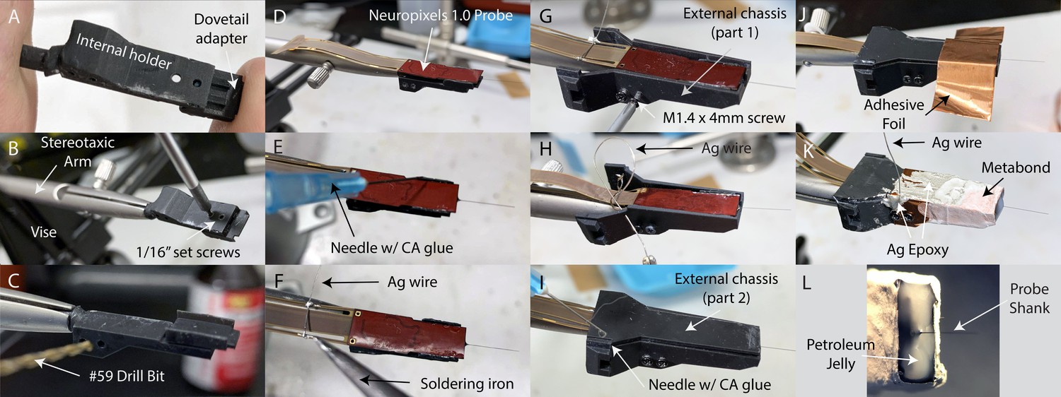
Implant construction.
(A) The internal holder and dovetail adapter are slid onto one another with a dovetail joint. (B) The internal holder is held in place during subsequent construction using a stereotaxic arm mounted on a tabletop with a vise. The internal holder and dovetail adapter are secured together with set screws. (C) The screw holes used to attach the internal holder to the external chassis are drilled out by hand with a pin vise, and the entire assembly is rotated such that the dovetail adapter’s flat platform is facing up. (D) The probe is laid flat against the platform, with the silicon spacer facing down. (E) The probe is glued in place by dropping several small drops of thin-viscosity cyanoacrylate (CA) glue in the gaps between the probe and platform. (F) A 10 cm length of bare silver (Ag) wire is soldered to pads on the flex cable to electrically connect the probe’s ground and external reference. (G) The first part of the external chassis is screwed onto the internal holder. (H) The silver wire is threaded through a small hole in the external chassis so that it can be connected to the animal ground during surgery. Note that this panel is mirror-reversed relative to the other panels to better illustrate the silver wire. (I) The second part of the external chassis is laid on top and glued to the first part with several drops of CA glue. (J) Adhesive copper foil tape is wrapped around the ventral portion of the assembly to shield the probe and seal any gaps between the two parts of the external chassis. (K) The implant assembly, fully constructed. The silver wire is electrically connected to the copper shield with silver epoxy. Silver epoxy is also applied where the copper shield overlapped itself, to ensure the adhesive backing did not prevent electrical contact. C and B Metabond (Parkell) is applied to the portion of the assembly to which dental cement will be applied during surgery (Figure 3B), to improve adhesion. Note that, like panel H, this panel is mirror-reversed for a better view of the silver wire. (L) The face of the implant from which the probe shank protrudes is sealed with petroleum jelly. The petroleum jelly is applied in liquid drops from a cautery.
Figure 3
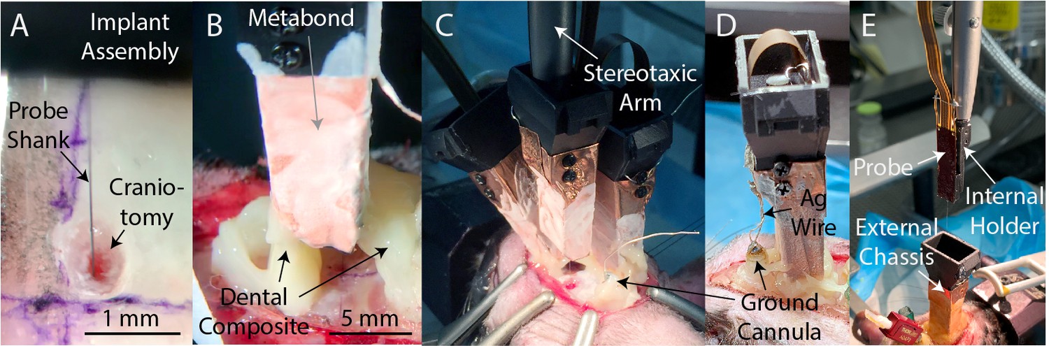
Implantation and explantation.
(A) A photograph of a probe being inserted into a craniotomy. (B) A photograph of a seal being formed around an implanted probe with dental composite (Absolute Dentin, Parkell). (C) A photograph of a third probe being lowered into the brain of subject A230. Note the steel ground cannula at the posterior edge of the exposed skull, soldered to a length (~5 cm) of silver wire and fixed in place with dental composite. (D) After implantation of all probes, the silver wire soldered to the ground cannula is soldered to the silver wires soldered to each probe, to provide a common ground for all probes. Dental acrylic (Duralay, Reliance Dental) was then applied to fully encapsulate the implant, including the silver wires. (E) A photograph of the explantation of a probe. The probe and internal holder have been lifted free from the implant using a stereotaxic arm while the external chassis remains bonded to the skull. Also visible is an interconnect for an optical fiber (red).
Figure 4 with 6 supplements

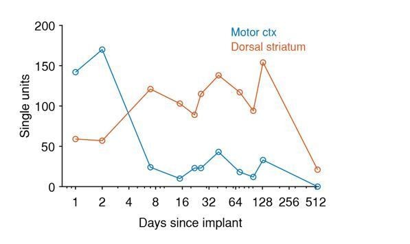
After an initial loss of units, spiking signals can be maintained >60 days in anterior, deeper brain regions.
(A) Recordings from the medial prefrontal cortex (encompassing the areas labelled in the Paxinos Brain Atlas as prelimbic cortex and medial orbital cortex) across three example animals. Each combination of marker and line types indicates one animal. (B) Recordings from motor cortex. (C) Recordings from nucleus accumbens. (D) The number of units recorded per electrode per session. Shading represents mean +/- 1 s.e.m. across recording sessions. The dashed line is the fit of a sum of two exponential decay terms, representing two subpopulations with different time constants of decay. (E) The number of single units. (F) To explore the dependence of signal stability on anatomical position, units were separated into two groups along either the dorsoventral (DV) axis or the anteroposterior (AP) axis. (G) The number of units recorded either more superficial to or deeper than 2 mm below the brain surface, normalized by the number of electrodes in the same region. (H) Similar to G, but showing the number of single units. (I) The model time constant is the inferred number of days after implantation when the count of units (or single units) declined to 1/e, or ~37%, of the count on the first day after implant. The 95% confidence intervals were computed by drawing 1000 bootstrap samples from the data. (J-L) Similar to G-I, but for data grouped according to their position along the anterior-posterior axis of the brain. (D-E) N = [12, 8, 20, 18, 32, 20, 13, 16] recording sessions for each bin. (G-H) DV [−10,–2] mm: N = [12, 8, 19, 18, 32, 20, 13, 16]; DV [−2, 0] mm: N = [6, 4, 11, 7, 14, 10, 8, 5]. (J-K) AP [−8, 0] mm: N = [2, 1, 5, 1, 8, 4, 1]; AP [0, 4] mm: N = [10, 7, 15, 17, 24, 16, 12, 16].
Figure 4—figure supplement 1
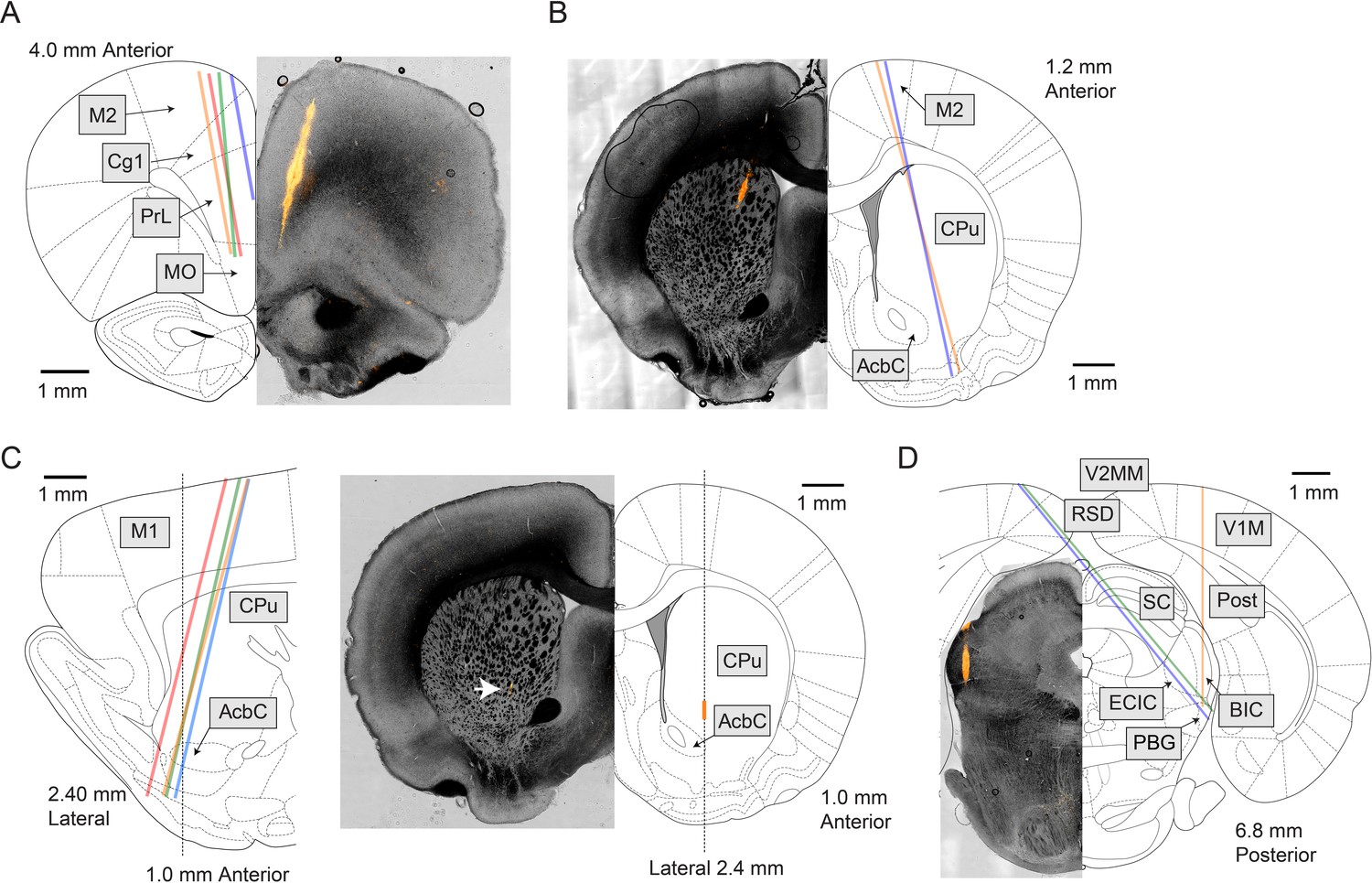
Example histological images of probe tracks.
(A) Four probes were implanted in the medial prefrontal cortex. The coordinates targeted (but not necessarily realized) were 4.0 mm anterior from Bregma, 1.0 mm lateral, and 4.2 mm deep, −10° in the coronal plane. (B) Two probes were implanted in anterior striatum and M2. The target coordinates were 1.9 mm anterior, 1.3 mm lateral, and 8.2 mm deep, and 15° in the coronal plane. (C) Four probes were implanted in M1 and anterior striatum. The target coordinates were 0.0 mm anterior, 2.4 mm lateral, 8.2 mm deep, and 15° in the sagittal plane. While the probe was tilted in the sagittal plane, histological slices were taken in the coronal plane. (D) Three probes were implanted in the midbrain with three different target coordinates: (1) 7.0 mm posterior, 3.0 mm lateral, and 5.8 mm deep. (2) 6.6 mm posterior, 1.6 mm lateral, and 7.8 mm deep, and −40° in the coronal plane. (3) 6.8 mm posterior, 1.7 mm lateral, and 8.0 mm deep, and −40° in the coronal plane. (A-D) Brain atlas was adapted from Paxinos and Watson, 2006. AcbC, accumbens nucleus, core. BIC, nucleus of the brachium of the inferior colliculus. Cg1, cingulate cortex, area 1. CPu, caudate putamen. ECIC, external cortex of the inferior colliculus. MO, medial orbital cortex. M1, primary motor cortex. M2, secondary motor cortex. PBG, parabigeminal nucleus. Post, postsubiculum. PrL, prelimbic cortex. RSD, retrosplenial dysgranular cortex. SC, superior colliculus. V1M, primary visual cortex, monocular. V2MM, secondary visual cortex, mediomedial. A positive angle in the coronal plane indicates that the probe tip was more lateral than the insertion site at the brain surface, and a positive angle in the sagittal plane indicates that the probe tip was more anterior than the insertion site.
Figure 4—figure supplement 2
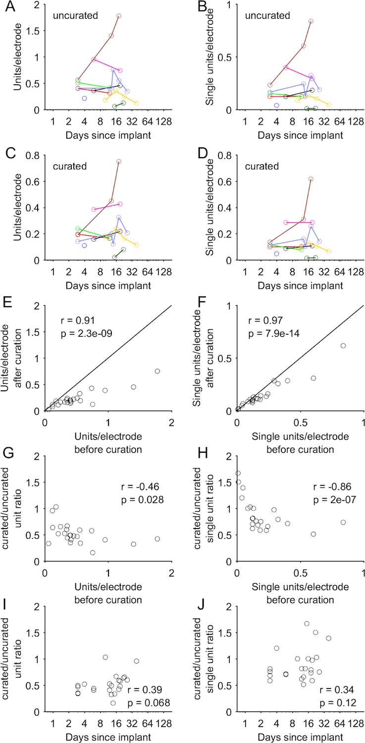
Comparison of yields before and after manual curation.
(A–B) Units and SUs (per electrode) identified by Kilosort2 before manual curation, shown as a function of time elapsed after implantation, for the subset of recording sessions that were manually curated (n = 25 sessions). Colors indicate sessions from the same implantations and banks. (C–D) Same data as in A,B after manual curation of the Kilosort2 output. Note the highly similar pattern of yield across sessions before and after manual curation. (E–F) Scatter plot directly comparing the yields (number of units or SUs per electrode) before and after manual curation. Nearly all points lie below the identity line but demonstrate a high degree of correlation, suggesting manual curation reduces the overall unit and SU number while having a minimal effect on the relative yields across sessions. Pearson r shown in these and subsequent plots, with a p-value reflecting a test of the null hypothesis of r = 0. (G–H) The ratio of units (and SUs) before versus after curation depends inversely on the number of units before curation. That is, a smaller fraction of units is removed (or in some cases, units are actually added) for sessions in which Kilosort2 identified a relatively small number of units. (I–J) The ratio of units (and SUs) before versus after curation depends weakly on the number of days elapsed since implantation, as would be expected given the relationship observed in G,H. This trend is non-significant, but suggests that curation could slightly alter the estimate of the time course of unit decline shown in Figure 4.
Figure 4—figure supplement 3
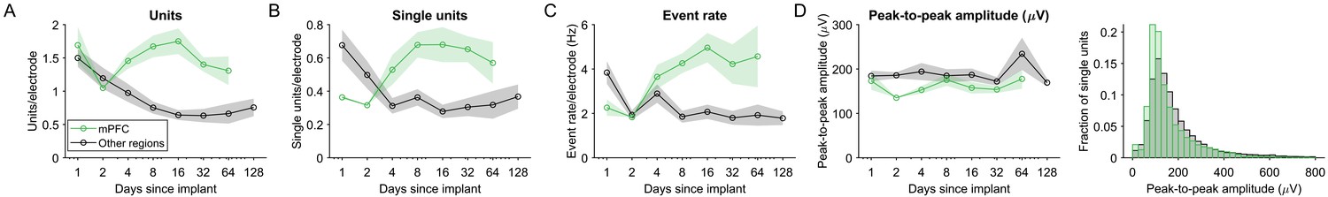
No degradation of spiking signals was detected over two months in rat medial prefrontal cortex (mPFC), the brain region in which the stability of spiking signals was examined in Jun et al., 2017.
mPFC was recorded from four probes (one probe/animal, N = (2, 1, 6, 3, 4, 6, 4) sessions, implanted 4.0 mm anterior to Bregma, 1.0 mm lateral, 10° in the coronal plane at the probe tip relative to DV axis) and from the electrodes of those probes located in prelimbic cortex or medial orbital cortex, as according to probe tracks in histological slices and referenced to Paxinos and Watson, 2006. This finding contrasts with the clear signal degradation at all other recording sites. N = (12, 8, 20, 18, 32, 20, 13, 16). (A) The number of single units normalized by the number of electrodes in that brain region. (B) The number of single units. (C) The event rate. (D) The average peak-to-peak amplitude of waveforms.
Figure 4—figure supplement 4
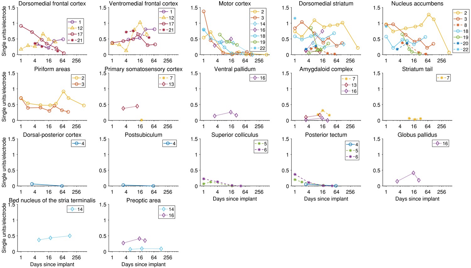
The yield in single units over time for each brain area and each implant.
Details about each implant can be found in Tables 1 and 2. Dorsomedial frontal cortex encompasses the areas named in the Paxinos and Watson brain atlas (Paxinos and Watson, 2006) as secondary motor cortex (M2) and cingulate cortex, area 1 (Cg1). Medial prefrontal cortex includes the areas prelimbic cortex (PrL) and medial orbital cortex (MO) in the atlas. Implants in both primary and motor cortices (M1 and M2) are grouped under ‘Motor cortex’. . Piriform areas include piriform cortex (Pir), dorsal endopiriform nucleus (DEn), and intermediate endopiriform nucleus (IEn). The amygdaloid body includes recording in anterior amygdaloid area (AA), anterior amygdaloid nucleus (ACo), lateral amygdaloid nucleus (dorsolateral region, LaDL), and basolateral amygdaloid nucleus (posterior region, BLP). Dorsal-posterior cortex includes recordings from primary visual cortex (monocular region, V1M) and retrosplenial granular cortex (region a, RSGa). The posterior tectum includes the external cortex of the inferior colliculus (ECIC) and the nucleus of the brachium of the inferior colliculus (BIC).
Figure 4—figure supplement 5
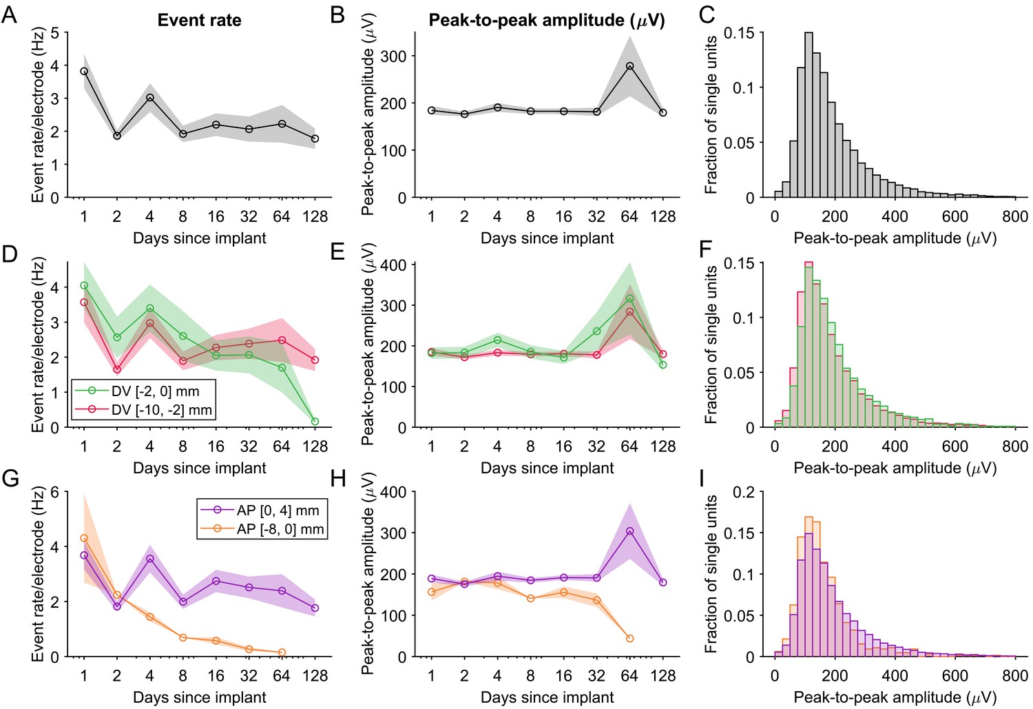
The event rate and peak-to-peak amplitudes.
(A) The event rate (rate of all spikes across units). Shading represents mean +/- 1 s.e.m. across recording sessions. The transient increase in event rate in the time bin including days 3–5 is in part due to non-identical subsets of animals being included in different time bins, resulting in event rate variability due to differences in implanted brain region or arousal levels across animals. (B) The average peak-to-peak amplitude of the waveforms across single units. (C) The distribution of the peak-to-peak amplitude of all single units. (D–F) Event rate and peak-to-peak amplitude of units recorded either more superficial to or deeper than 2 mm below the brain surface, normalized by the number of electrodes in the same region. (G–I) Similar as (D–F), but for data grouped according to their position along the anterior-posterior axis of the brain.
Figure 4—figure supplement 6
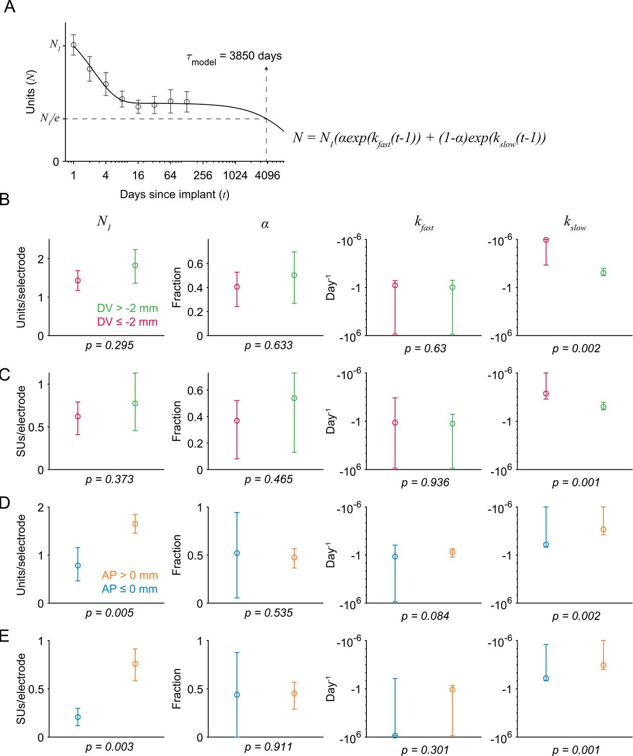
Coefficient estimates of the sum-of-exponentials model used to describe unit loss over time.
The model postulates that the number of units (N) across days after implant (t) depended on exponential decay from the unit count on the first day after surgery (N1). The term α is the fraction of the population whose exponential decay is parametrized by the change rate kfast, and the remaining fraction (1-α) decays with a slower (i.e. larger) time constant kslow. (A) The model time constant (𝜏model) is the inferred time when the unit count is 1/e of the initial value. Markers and error bar indicate mean +/- 1 s.e.m. Solid line indicates the model fit. (B) Fits to the number of units recorded either more superficial to (green) or deeper than (red) 2 mm below the brain surface. The p-value was computed from a two-tailed bootstrap test. For each parameter, the p-value indicates the probability of the observed difference in the estimate between the model fit to the superficial units and the model fit to the deeper units, under the null hypothesis that the distributions of unit counts from superficial and deeper electrodes are identical. (C) Same as B, but for the number of single units. (D) Fits to the number of units recorded either more anterior to (orange) or posterior to (blue) Bregma. (E) Same as D, but for single units.
Figure 5 with 1 supplement
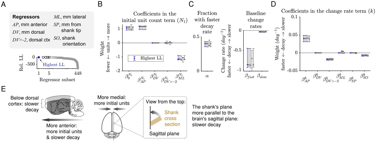
The initial unit count depends on the AP and ML positions, and the rate of decay depends on the AP position, whether an electrode is in dorsal cortex, and the shank orientation.
(A) A sum-of-exponentials regression (SoER) model was fit to the number of units recorded from each electrode in each session (N = 57,586 recordings) to infer the relationship between experimental factors and unit loss over time. Continuous regressors AP, DV, ML, SP, and SO indicate an electrode’s position in millimeters anterior, dorsal, lateral, and from the shank tip, and the orientation (in degrees) between the shank’s plane from the brain’s sagittal plane, respectively. Categorical regressors DV>-2 indicate whether an electrode is in the dorsal cortex. Model variants with different subsets of regressors were ordered by relative out-of-sample log-likelihood (LL). The five subsets with the highest LL are shown in subsequent panels. (B) Coefficients in the equation term indicating the initial unit count (N1) from the five regressors subsets with the highest LL. Initial unit count consistently depends on AP and ML (orange), which are included and significantly nonzero in the top five models. Error bars indicate 95% bootstrap confidence intervals. The range of all regressors is normalized to be [0,1] to facilitate comparison. The original range of the regressors were AP [−7.40, 4.00], DV [−9.78,–0.01], ML [0.29, 5.59], SP [0.02, 7.68], SO [0, 90]. (C) About 40% (α) of the units disappeared rapidly with a baseline change rate of −0.87 (kfast), and the remaining disappeared more slowly with a baseline change rate of −0.03 (kslow). (D) Change rates depended consistently on the regressors AP, DV>-2 (whether the unit was in dorsal cortex), and SO (angle between the shank’s plane and the brain’s sagittal plane), which are included and have a significantly nonzero coefficient in the top five models. (E) A graphical summary of the modeling results.
Figure 5—figure supplement 1
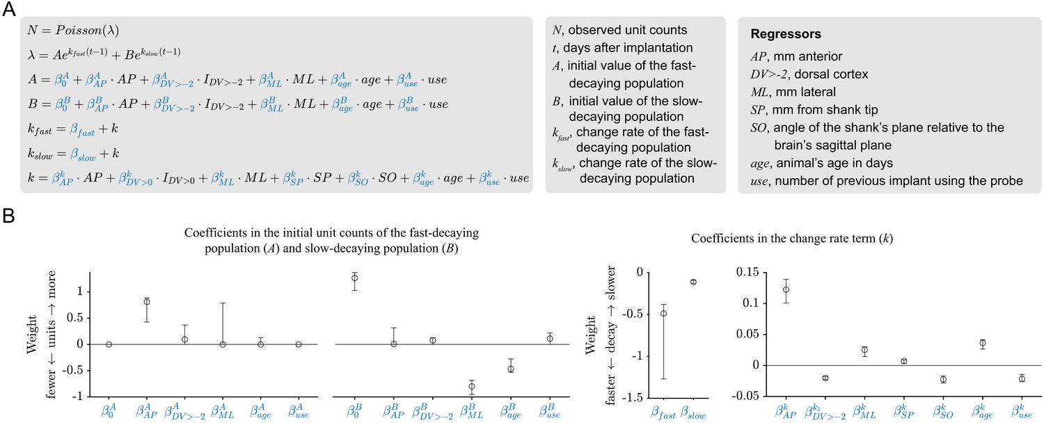
The results of the sum-of-exponentials regression (SoER) model are corroborated by the results of an elaborated SoER model.
(A) Two additional regressors (the animal’s age and the number of times a probe was previously used for chronic implantation) are added to the elaborated model. The initial unit counts of the fast- and slow-decaying population in the basic model depend on separate linear combinations of the regressors (A and B), whereas in the basic model they depended on a single linear combination of the regressors (N) and a scaling parameter (α). The variable Y is a vector of observed unit count on each electrode pooled across all recordings and is assumed to follow a Poisson distribution, and the λ parameter of the Poisson distribution is a sum of two exponentials. The parameter t is the number of days after implantation, A is the initial unit count of the fast-decaying population, and B is the initial unit count of the slow-decaying population. The parameters kfast and kslow are the exponential change rates of the fast- and slow-decaying populations, respectively. Note that these two parameters differ by a constant offset (βkfast – βkslow) and depend on the same linear combination of the regressors (k). (B) Maximum-likelihood estimates of the model parameters. The model was fit using L1 (LASSO) regularization to sparify coefficient estimates. Error bars indicate bootstrapped 95% confidence interval. Similar to the basic model, the initial unit counts depended on the regressors AP and ML and the changes rates depended on the regressors AP, DV>-2, and SO.
Figure 6
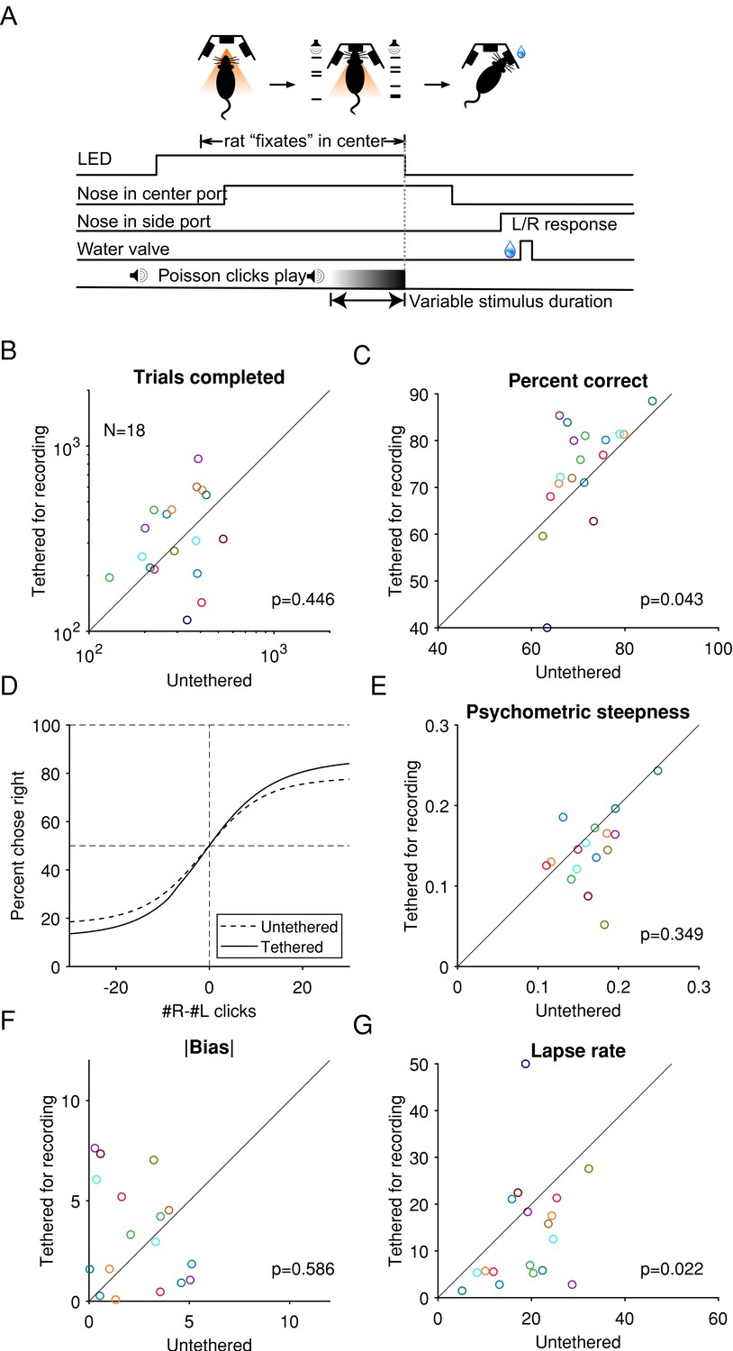
While tethered for Neuropixel recording without a cable commutator, rats performed a cognitively demanding task at a level similar to when they were untethered.
(A) Task schematic: rats hold their nose in the center port while listening to two concurrent streams of auditory clicks, one from a loudspeaker to its left and the other to its right. At the end of the stimulus, the rat receives a reward if it oriented toward the port on the side where more clicks were played. Reproduced from Brunton et al., 2013. (B) The median number of trials completed by an animal in each training or recording session, compared between tethered and untethered. Each marker indicates an animal. p-Values are based on the null hypothesis that the median difference between paired observations is zero and calculated using the Wilcoxon signed-rank test. (C) The percentage of trials when an animal responded correctly. (D) Logistic curves fitted to data pooled across from all animals. (E) Comparison of the behavioral psychometric curves’ sensitivity parameter, which controls the steepness of the logistic function. (G) Absolute value of the bias parameter. (F) The average of the lapse rate. A larger lapse indicates a larger fraction of trials when the animal was not guided by the stimulus or a decreased ability to take advantage of large click differences.
© 2013, AAAS permissions. From Brunton et al., 2013. Reprinted with permission from AAAS. It is not covered by the CC-BY 4.0 licence and further reproduction of this panel would need permission from the copyright holder.
Figure 7
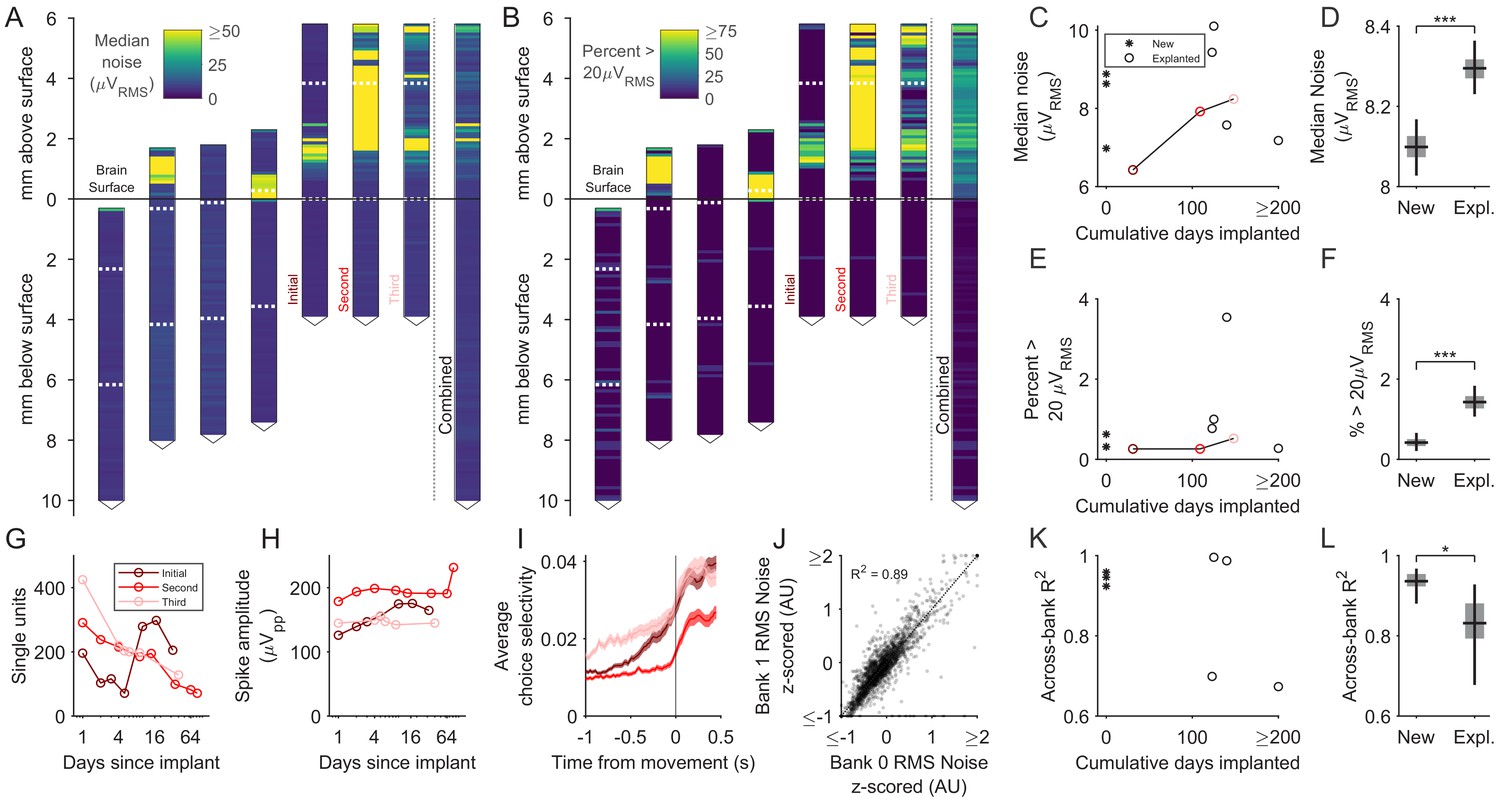
Explanted probes and unimplanted probes have similar input-referred noise and can acquire neural signals of similar quality.
(A) Shank map showing the RMS input-referred noise (i.e. noise divided by gain), measured in saline, along the entire shank of explanted probes, aligned and ordered according to their implanted depth. Note high noise confined to the part of the shank above the brain surface, where silicone elastomer and/or petroleum jelly were applied during surgery. These sites are excluded from the data contributing to the subsequent panels. Combined data across explanted probes is at the right. Note that the three rightmost shank maps come from repeated explantations of the same probe. Dashed horizontal white lines indicate the boundaries between banks. (B) Same as A, but showing the percentage of recording sites with RMS noise >20μV. (C) The median noise, shown separately by probe as a function of time implanted. Measurements from one probe that was implanted in three different animals are connected by a line. (D) Box plot showing slightly higher median noise across recording sites of explanted probes compared to new probes (p<10−4, bootstrap test for difference in median noise). Boxes and whiskers indicate the 50% and 95% bootstrap CI, respectively. Bootstrapping performed by resampling electrodes. (E) The percentage of recording sites with a noise value greater than 20μVRMS shown separately by probe as a function of time implanted. (F) Box plot showing that the fraction of recording sites with a noise value greater than 20μVRMS was slightly higher in explanted probes (p<10−4, bootstrap test for difference in fraction of noisy electrodes). Boxes and whiskers indicate the 50% and 95% bootstrap CI, respectively. Bootstrapping performed by resampling electrodes. (G–H) Signal quality of the same probe implanted in the medial frontal cortex of three separate animals. (I) Choice selectivity averaged across units did qualitatively change across successive implants. Shading indicates mean +/- 1 s.e.m. (J) Noise was highly similar across pairs of recording sites on separate banks that were addressed by the same acquisition channel (n = 6544 recording sites across new and explanted probes). Scatter plot shows RMS noise values for electrode pairs in banks 0 and 1 that were implanted below the brain surface, z-scored in groups defined by probe and bank. Data points are shown with transparency, such that regions containing more of them appear darker. (K). The across-bank noise similarity (R2), as computed in J, shown separately by probe as a function of time implanted. Note that the probe implanted three times is not included here, since bank one was never inserted into the brain. (L) Box plot showing the across-bank noise similarity (R2) was lower in explanted probes (p=0.033, bootstrap test for difference in R2). Boxes and whiskers indicate the 50% and 95% bootstrap CI, respectively. Bootstrapping performed by resampling electrodes.
Author response image 1
Tables
Table 1
All implantations.
Note that rats A230, A241, and A243 had multiple probes implanted simultaneously. A positive angle in the coronal plane indicates that the probe tip was more lateral than the insertion site at the brain surface, and a positive angle in the sagittal plane indicates that the probe tip was more anterior than the insertion site. [1] Could not be successfully explanted, most likely because no petroleum jelly was applied at the base of the implant to mitigate blood entering into the space between the holder and the chassis and bonding them together. [2] Implant detached before explantation could be attempted. This only occurred for rats that had undergone multiple sequential surgeries, and only after 100 days or more from the initial surgery. Skull degradation was observed in these cases. [3] Probe was damaged during recording before explantation could be attempted.
| Implant # | Date implanted | Animal ID | Probe serial number | Coordinates of the insertion site relative to bregma | Insertion depth (mm) | Angle in the coronal plane (°) | Angle in the sagittal plane (°) | Shank plane angle relative to the sagittal plane (°) | Animal’s age at the time of implant (day) | Number of times the probe was previously implanted | Holder version | Explantation attempted | Reusable after explantation | |
|---|---|---|---|---|---|---|---|---|---|---|---|---|---|---|
| AP (mm) | ML (mm) | |||||||||||||
| 1 | 4/6/18 | T176 | 619040938 | 4 | 1 | 4.2 | −10 | 0 | 90 | 493 | 0 | Early | Yes, 96 days post-implant | No [1] |
| 2 | 5/24/18 | T181 | 17131306102 | 1.9 | 1.3 | 8.2 | 15 | 0 | 0 | 238 | 0 | Yes, 536 days post-implant | ||
| 3 | 5/30/18 | T182 | 17131311881 | 1.9 | 1.3 | 8.2 | 15 | 0 | 0 | 244 | 0 | Yes, 125 days post-implant | Yes | |
| 4 | 1/20/19 | T179 | 17131311342 | −7 | 3 | 5.8 | 0 | 0 | 90 | 505 | 0 | Yes, 176 days post-implant | No [3] | |
| 5 | 4/22/19 | T196 | 17131312042 | −7.2 | 1.7 | 8 | −40 | 0 | 90 | 410 | 0 | Yes, 135 days post-implant | Yes | |
| 6 | 5/6/19 | T209 | 17131311352 | −7.4 | 1.6 | 7.8 | −40 | 0 | 90 | 370 | 0 | Yes, 122 days post-implant | Yes | |
| 7 | 5/20/19 | A242 | 17131311621 | −2.35 | 4.95 | 7.6 | 5 | 0 | 0 | 258 | 0 | No [3] | — | |
| 8 | 5/22/19 | K265 | 17131311562 | 1.9 | 0.8 | 7 | 20 | 0 | 90 | 656 | 0 | Yes, 53 days post-implant | No [1] | |
| 9 | 7/2/19 | A230 | 17131308411 | 2.2 | 5 | 8.6 | 5 | 0 | 0 | 420 | 0 | Current | No [3] | — |
| 10 | 7/2/19 | A230 | 17131308571 | 0.8 | 4 | 6.6 | −2 | 0 | 0 | 420 | 0 | |||
| 11 | 7/2/19 | A230 | 18005106831 | 4 | 0.5 | 7.5 | 26 | −29 | 45 | 420 | 0 | |||
| 12 | 8/3/19 | T212 | 17131312432 | 4 | 1 | 4.2 | −10 | 0 | 90 | 459 | 0 | Yes, 31 days post-implant | Yes | |
| 13 | 9/11/19 | A241 | 18194823302 | −0.6 | 4 | 10 | −2 | 0 | 0 | 372 | 0 | Yes, 140 days post-implant | Yes | |
| 14 | 9/11/19 | A241 | 18194823631 | 0.7 | 2.15 | 10 | 2 | 0 | 0 | 372 | 0 | No [3] | — | |
| 15 | 9/13/19 | A243 | 18194823211 | −0.6 | 4 | 9.45 | −2 | 0 | 0 | 374 | 0 | No [3] | — | |
| 16 | 9/13/19 | A243 | 18194824132 | 0.7 | 2.45 | 9 | 0 | 0 | 0 | 374 | 0 | |||
| 17 | 11/14/19 | T224 | 17131312432 | 4 | 1 | 4.2 | −10 | 0 | 90 | 520 | 1 | Yes, 81 days post-implant | Yes | |
| 18 | 11/17/19 | T219 | 18194824092 | 1 | 2.4 | 8 | 0 | 15 | 90 | 523 | 0 | No [2] | — | |
| 19 | 11/22/19 | T223 | 19051017162 | 1 | 2.4 | 7.9 | 0 | 15 | 90 | 528 | 0 | |||
| 20 | 2/4/20 | A249 | 18194819132 | 2.2 | 2.1 | 6.8 | 0 | −5 | 90 | 393 | 0 | Recording ongoing | — | |
| 21 | 2/6/20 | T249 | 17131312432 | 4 | 1.2 | 4.2 | −10 | 0 | 90 | 338 | 2 | Yes, 39 days post-implant | Yes | |
| 22 | 3/14/20 | T227 | 18194819542 | 1 | 2.4 | 8.4 | 0 | 15 | 90 | 557 | 0 | No [2] | — | |
Table 2
The brain areas recorded in each implant.
The implant numbers are the same as in Table 1 and in Figure 4—figure supplement 4. No recording was obtained from implants #9, 11, 15 due to poor signal quality.
| Brain area | Implant # | Animal ID | Probe serial number | Animal’s age on the time of implant (day) | Number of times the probe was previously implanted | Insertion depth (mm) | Number of electrodes in the brain area | Shank plane angle relative to the sagittal plane (°) | Center of mass of electrodes in the brain area (mm) | ||
|---|---|---|---|---|---|---|---|---|---|---|---|
| AP | ML | DV | |||||||||
| Dorsomedial frontal cortex | 1 | T176 | 619040938 | 493 | 0 | 4.2 | 170 | 0 | 4 | 0.8 | -1.1 |
| 12 | T212 | 17131312432 | 459 | 0 | 4.2 | 174 | 0 | 4 | 0.8 | -1 | |
| 17 | T224 | 17131312432 | 520 | 1 | 4.2 | 174 | 0 | 4 | 0.8 | -1 | |
| 21 | T249 | 17131312432 | 338 | 2 | 4.2 | 186 | 0 | 4 | 1 | -1.1 | |
| Ventromedial frontal cortex | 1 | T176 | 619040938 | 493 | 0 | 4.2 | 213 | 0 | 4 | 0.5 | -3 |
| 12 | T212 | 17131312432 | 459 | 0 | 4.2 | 209 | 0 | 4 | 0.5 | -2.9 | |
| 17 | T224 | 17131312432 | 520 | 1 | 4.2 | 209 | 0 | 4 | 0.5 | -2.9 | |
| 21 | T249 | 17131312432 | 338 | 2 | 4.2 | 197 | 0 | 4 | 0.7 | -3 | |
| Motor cortex | 2 | T181 | 17131306102 | 238 | 0 | 8.2 | 214 | 90 | 1.9 | 1.7 | -1.4 |
| 3 | T182 | 17131311881 | 244 | 0 | 8.2 | 214 | 90 | 1.9 | 1.7 | -1.4 | |
| 14 | A241 | 18194823631 | 372 | 0 | 10 | 27 | 90 | 0.7 | 2.2 | -2.2 | |
| 16 | A243 | 18194824132 | 374 | 0 | 9 | 48 | 90 | 0.7 | 2.4 | -1.4 | |
| 18 | T219 | 18194824092 | 523 | 0 | 8 | 241 | 0 | 1.3 | 2.4 | -1.3 | |
| 19 | T223 | 19051017162 | 528 | 0 | 7.9 | 241 | 0 | 1.3 | 2.4 | -1.2 | |
| 22 | T227 | 18194819542 | 557 | 0 | 8.4 | 241 | 0 | 1.4 | 2.4 | -1.7 | |
| Dorsomedial striatum | 2 | T181 | 17131306102 | 238 | 0 | 8.2 | 198 | 90 | 1.9 | 2.3 | -3.8 |
| 3 | T182 | 17131311881 | 244 | 0 | 8.2 | 236 | 90 | 1.9 | 2.3 | -3.7 | |
| 8 | K265 | 17131311562 | 656 | 0 | 7 | 234 | 0 | 1.9 | 2.2 | -3.9 | |
| 10 | A230 | 17131308571 | 420 | 0 | 6.6 | 184 | 90 | 0.8 | 3.9 | -3.5 | |
| 13 | A241 | 18194823302 | 372 | 0 | 10 | 199 | 90 | -0.6 | 3.9 | -3.7 | |
| 14 | A241 | 18194823631 | 372 | 0 | 10 | 219 | 90 | 0.7 | 2.3 | -3.5 | |
| 16 | A243 | 18194824132 | 374 | 0 | 9 | 250 | 90 | 0.7 | 2.4 | -3.3 | |
| 18 | T219 | 18194824092 | 523 | 0 | 8 | 270 | 0 | 2 | 2.4 | -3.8 | |
| 19 | T223 | 19051017162 | 528 | 0 | 7.9 | 270 | 0 | 2 | 2.4 | -3.7 | |
| 20 | A249 | 18194819132 | 393 | 0 | 6.8 | 256 | 0 | 1.8 | 2.1 | -4 | |
| 22 | T227 | 18194819542 | 557 | 0 | 8.4 | 270 | 0 | 2.1 | 2.4 | -4.2 | |
| Nucleus accumbens | 2 | T181 | 17131306102 | 238 | 0 | 8.2 | 191 | 90 | 1.9 | 2.9 | -5.9 |
| 3 | T182 | 17131311881 | 244 | 0 | 8.2 | 176 | 90 | 1.9 | 2.9 | -5.9 | |
| 8 | K265 | 17131311562 | 656 | 0 | 7 | 149 | 0 | 1.9 | 2.9 | -5.7 | |
| 18 | T219 | 18194824092 | 523 | 0 | 8 | 255 | 0 | 2.7 | 2.4 | -6.3 | |
| 19 | T223 | 19051017162 | 528 | 0 | 7.9 | 255 | 0 | 2.7 | 2.4 | -6.2 | |
| 20 | A249 | 18194819132 | 393 | 0 | 6.8 | 127 | 0 | 1.7 | 2.1 | -5.9 | |
| 22 | T227 | 18194819542 | 557 | 0 | 8.4 | 255 | 0 | 2.8 | 2.4 | -6.7 | |
| Piriform areas | 2 | T181 | 17131306102 | 238 | 0 | 8.2 | 115 | 90 | 1.9 | 3.2 | -7.2 |
| 3 | T182 | 17131311881 | 244 | 0 | 8.2 | 106 | 90 | 1.9 | 3.2 | -7.2 | |
| Primary somatosensory cortex | 7 | A242 | 17131311621 | 258 | 0 | 7.6 | 353 | 90 | -2.3 | 5.1 | -1.8 |
| 13 | A241 | 18194823302 | 372 | 0 | 10 | 58 | 90 | -0.6 | 3.9 | -2.4 | |
| Ventral pallidum | 16 | A243 | 18194824132 | 374 | 0 | 9 | 99 | 90 | 0.7 | 2.5 | -6.6 |
| Amygdaloid complex | 7 | A242 | 17131311621 | 258 | 0 | 7.6 | 70 | 90 | -2.4 | 5.6 | -7 |
| 13 | A241 | 18194823302 | 372 | 0 | 10 | 208 | 90 | -0.6 | 3.7 | -8.7 | |
| 16 | A243 | 18194824132 | 374 | 0 | 9 | 69 | 90 | 0.7 | 2.5 | -8.5 | |
| Striatum tail | 7 | A242 | 17131311621 | 258 | 0 | 7.6 | 209 | 90 | -2.3 | 5.4 | -5.1 |
| Dorsal-posterior cortex | 4 | T179 | 17131311342 | 505 | 0 | 5.8 | 109 | 0 | -7 | 3 | -0.9 |
| Postsubiculum | 4 | T179 | 17131311342 | 505 | 0 | 5.8 | 112 | 0 | -7 | 3 | -2.4 |
| Superior colliculus | 5 | T196 | 17131312042 | 410 | 0 | 8 | 239 | 0 | -7.2 | 1.6 | -4 |
| 6 | T209 | 17131311352 | 370 | 0 | 7.8 | 190 | 0 | -7.4 | 1.4 | -3.6 | |
| Posterior tectum | 4 | T179 | 17131311342 | 505 | 0 | 5.8 | 259 | 0 | -7 | 3 | -4.3 |
| 5 | T196 | 17131312042 | 410 | 0 | 8 | 144 | 0 | -7.2 | 2.9 | -5.4 | |
| 6 | T209 | 17131311352 | 370 | 0 | 7.8 | 193 | 0 | -7.4 | 2.7 | -5.1 | |
| Globus pallidus | 16 | A243 | 18194824132 | 374 | 0 | 9 | 139 | 90 | 0.7 | 2.5 | -5.4 |
| Bed nucleus of the stria terminalis | 14 | A241 | 18194823631 | 372 | 0 | 10 | 221 | 90 | 0.7 | 2.3 | -5.7 |
| Preoptic area | 14 | A241 | 18194823631 | 372 | 0 | 10 | 299 | 90 | 0.7 | 2.4 | -8.3 |
| 16 | A243 | 18194824132 | 374 | 0 | 9 | 100 | 90 | 0.7 | 2.5 | -7.6 | |
Key resources table
| Reagent type (species) or resource | Designation | Source or reference | Identifiers | Additional information |
|---|---|---|---|---|
| Strain, strain background (species) | Hla(LE)CVF (Rattus norvegicus) | Hilltop Lab Animals | Hla(LE)CVF | Long-evans rat |
| Commercial assay or kit | C and B Metabond Quick Adhesive Cement System | Parkell | S380 | |
| Chemical compound, drug | Absolute Dentin dual-cure core composite | Parkell | S305 | |
| Vetbond Tissue Adhesive | 3M | 70200742529 | ||
| Dil Stain | Thermo Fisher Scientific | D282 | 1 mg/mL in isopropyl alcohol | |
| DOWSIL 3–4680 Silicone Gel Kit | DOW | 3–4860 | ||
| Kwiksil | World Precision Instruments | KWIK-SIL | ||
| Black photopolymer resin | Formlabs | RS-F2-GPBK-04 | ||
| Tough photopolymer resin | Formlabs | RS-F2-TOTL-05 | ||
| Software, algorithm | SpikeGLX | https://billkarsh.github.io/SpikeGLX/ | ||
| Kilosort2 | https://github.com/MouseLand/Kilosort2 | Tag: ‘1.0’ (Dec 16, 2019) | ||
| Bcontrol | https://brodylabwiki.princeton.edu/bcontrol/index.php?title=Main_Page | |||
| Other | 3D printed implant assembly | This paper | https://github.com/Brody-Lab/chronic_neuropixels/tree/master/Holder20CAD20Files | |
| Stereolithography printer | Formlabs | Form two or Form 3 | ||
| Slit corrugated sleeving | McMaster | 2569K93 | ||
| Neuropixel 1.0 Probe with a flat silicon cap | IMEC | PRB_1_4_0480_1 | ||
| Model 1766-AP Cannula Holder | Kopf | 1766-AP | ||
| Silver wire 0.01’/254 µm diameter | A-M Systems | 782500 | ||
| Infusion cannula | Invivo1 | C315GMN/SPC | ||
| Cyanoacrylate accelerator | Pacer Technology | PT-29 | ||
| Conductive copper foil electrical tape | McMaster | 76555A714 | ||
| Low-temperature cautery | Bovie | AA00 | ||
| Tergazyme | Sigma-Aldrich | Z273287-11KG | ||
| PXI Chassis | NI | PXIe-1071 | ||
| PXI Multifunction I/O Module | NI | PXI-6133 | ||
| Noise Rejecting, Shielded BNC Connector Block | NI | BNC-2110 | ||
| PXI Waveform Generator | NI | PXIe-5413 | ||
| RF attenuator | Pomona Electronics | 4108–20 DB |
Additional files
Download links
A two-part list of links to download the article, or parts of the article, in various formats.
Downloads (link to download the article as PDF)
Open citations (links to open the citations from this article in various online reference manager services)
Cite this article (links to download the citations from this article in formats compatible with various reference manager tools)
An approach for long-term, multi-probe Neuropixels recordings in unrestrained rats
eLife 9:e59716.
https://doi.org/10.7554/eLife.59716


