Figures and data in Development of visual motion integration involves coordination of multiple cortical stages

Figures
Tables
Additional files

8 figures, 2 tables and 1 additional file

Figures

Figure 1 with 1 supplement

Download asset Open asset

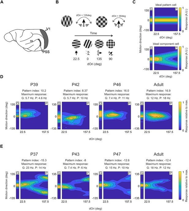
Pattern and component cells are found in PSS across all ages tested.

(A) Sagittal view of the ferret brain indicating the location of PSS and V1 (ss: suprasylvian sulcus). (B) Top: Plaid stimuli with different angles between the component directions (dOri). Bottom: Illustration of the streaming stimulus paradigm: Plaids of different dOri values and directions were presented along with gratings moving in different directions (see Materials and methods). (C) Simulated responses of an ideal pattern (top) and component cell (bottom) to gratings and plaids. In this and the following figures, the small contour plot for each cell (labeled ‘G’) represents the responses to gratings only. The large 2D contour plot (labeled ‘P’) summarizes responses to all plaids as a function of dOri and direction. In both plots, direction is relative to the cell’s preferred grating direction. For ‘G’, direction refers to the grating direction; for ‘P’, direction refers to the pattern direction (i.e. the perceived direction of the plaid). ‘G’ and ‘P’ are independently normalized by their respective maximum to help with visualization of the tuning properties. An ideal pattern cell would respond maximally to plaid stimuli moving in its preferred direction. An ideal component cell would respond maximally whenever one plaid component moves in the preferred direction, resulting in a response profile with a characteristic ‘V’-shape. For the ideal cells, resposes were scaled so that the area under the direction curve remained constant across dOri values. As a consequence, the responses for the ideal component cell change with dOri (because different number of directions evoke strong responses). All other dOri dependencies were ignored in this illustration. (D) Responses of example PSS neurons classified as pattern cells (see Materials and methods for classification procedure) in ferrets of different ages. For each neuron, we list the pattern index, as well as the maximum response rate evoked by gratings (G) and plaids (P) (otherwise same format as in (C)). (E) Responses of example PSS component cells in ferrets of different age (same format as (D)).

Figure 1—figure supplement 1

Download asset Open asset

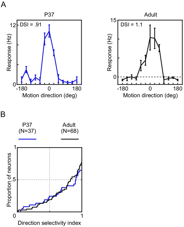
PSS direction selectivity is mature at P37.

(A) Direction tuning curves of example PSS neurons at P37 (left) and in an adult animal (right), as measured with gratings. The DSI is indicated for each neuron (see Materials and methods). Error bars indicate ± SEM. (B) Cumulative distribution plots of the PSS direction selectivity index at P37 and in adult ferrets. Results indicate mature levels of direction tuning at P37. For statistical comparison of data across groups, see Table 1.

Figure 2 with 1 supplement

Download asset Open asset

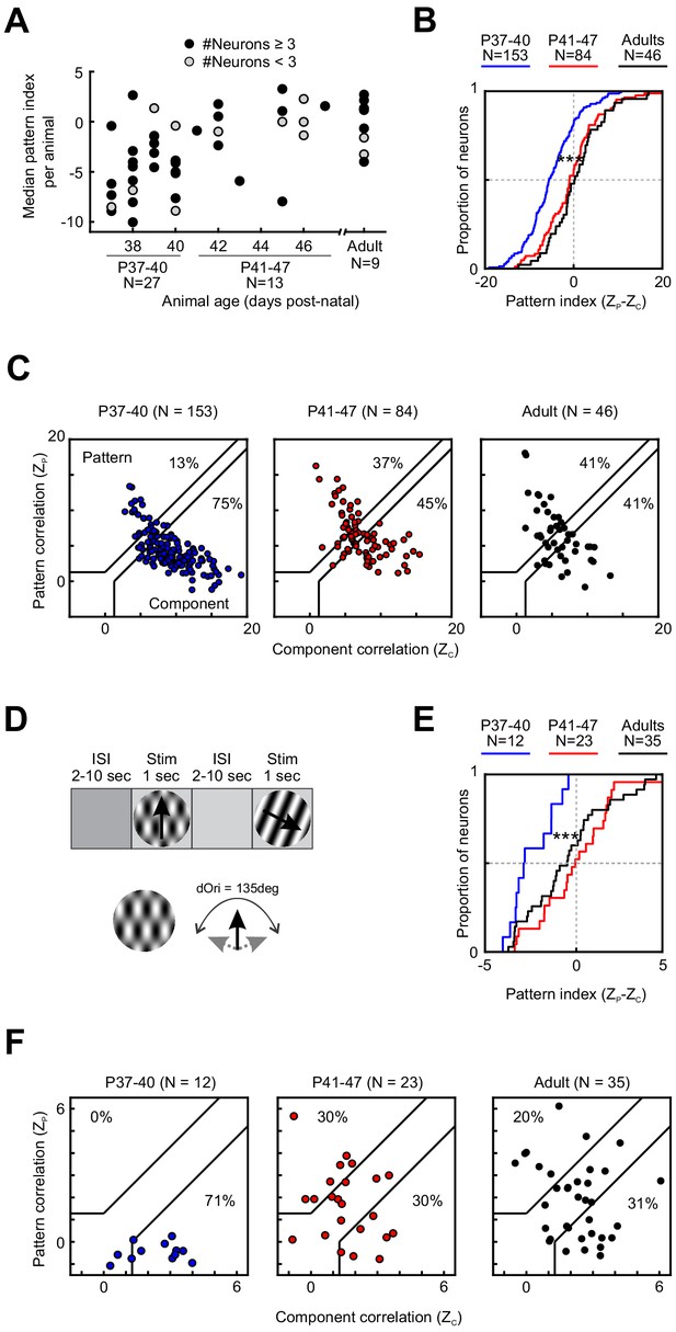
Motion integration in PSS matures around P41.

(A) Median PSS pattern index for each animal included in the study, plotted as a function of age. Gray dots represent animals that yielded one to two neurons, black dots represent animals with data for at least three neurons. (B) Cumulative distributions for pattern indices in different age groups. For further information on statistical tests for this and all following plots, see Table 1. ***p<0.001. (C) Pattern versus component correlations for PSS neurons in animals from different age groups. For each neuron, Z_P is plotted against Z_C. Black lines indicate the category boundaries used to classify cells into pattern, unclassified, and component cells. Percentages indicate the portion of neurons falling into the component and pattern categories. (D) Top: Illustration of the classic stimulus presentation paradigm, in which stimuli were presented for 1 s, and stimulus presentations were interleaved by 2–10 s of inter-stimulus interval. Bottom: Example plaid stimulus with 135 degrees of difference between the component directions. (E) Same as (B), but for pattern indices computed from responses to plaids presented in the classic stimulus paradigm as shown in (D). ***p<0.001. (F) Same as (C), but for pattern and component correlations computed based on the classic stimulus paradigm as shown in (D).

Figure 2—source data 1 Neuron-by-neuron metrics for Figure 2 and Figure 2—figure supplement 1.: https://cdn.elifesciences.org/articles/59798/elife-59798-fig2-data1-v2.xlsx
Download elife-59798-fig2-data1-v2.xlsx

Figure 2—figure supplement 1

Download asset Open asset

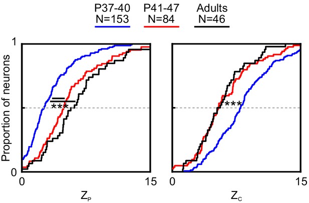
Changes in pattern and component correlation contribute to the developmental increase in pattern index.

Cumulative distributions of pattern (left) and component (right) correlations for PSS cells recorded in different age groups. Data recorded using the streaming stimulus paradigm. For statistical comparisons see Table 1. ***p<0.001.

Figure 3

Download asset Open asset

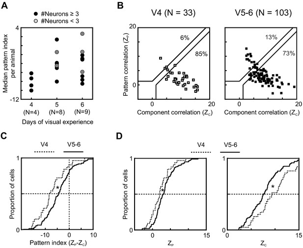
Longer visual experience results in a higher degree of PSS motion integration.

(A) Median PSS pattern index for each animal aged P37–40, plotted as a function of visual experience. Gray dots represent animals that yielded 1–2 neurons, and black dots represent animals with data for at least three neurons. (B) Pattern versus component correlations at P37–40 split according to visual experience (same plot format as Figure 2C). (Left) Animals with 4 days of visual experience. (Right) Animals with 5–6 days of visual experience. (C) Cumulative distributions of pattern indices for PSS cells in kits with 4 days (V4, dashed line) or 5–6 days (V5-6, solid line) of visual experience. *p<0.05. (D) Cumulative distributions for component correlation (left) and pattern correlation (right) for the two groups. *p<0.05.

Figure 3—source data 1 Neuron-by-neuron metrics for Figure 3.: https://cdn.elifesciences.org/articles/59798/elife-59798-fig3-data1-v2.xlsx
Download elife-59798-fig3-data1-v2.xlsx

Figure 4 with 1 supplement

Download asset Open asset

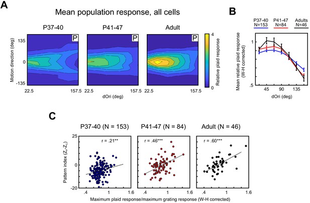
Responses of PSS neurons to plaid stimuli become increasingly modulated by dOri with development, especially in pattern cells.

(A) Average 2D profile of PSS responses to plaids at different ages (plotted in same format as Figure 1D–E). Average response profiles were computed by normalizing the data for each neuron by its mean grating response, shifting responses in direction space to center the preferred direction at 0 deg, and averaging across all neurons in each age group. (B) Average relative plaid response as a function of dOri. The average relative plaid response shown here was computed by averaging the relative plaid responses shown in (A) across all directions at each dOri. All data were transformed using a Wilson–Hilferty transformation to achieve a normal distribution at each dOri value. Error bars: ± SEM. For statistical comparisons of data across age groups, see Table 1. (C) Ratio between the maximum response to plaids of dOri = 90 deg and the maximum response to gratings versus the pattern index for all PSS neurons at different ages. Dashed lines indicate linear fits, r the correlation coefficient. Data are shown after a Wilson–Hilferty transformation. **p<0.01. ***p<0.001.

Figure 4—source data 1 Neuron-by-neuron metrics for Figure 4 and Figure 5—figure supplement 1.: https://cdn.elifesciences.org/articles/59798/elife-59798-fig4-data1-v2.xlsx
Download elife-59798-fig4-data1-v2.xlsx

Figure 4—figure supplement 1

Download asset Open asset

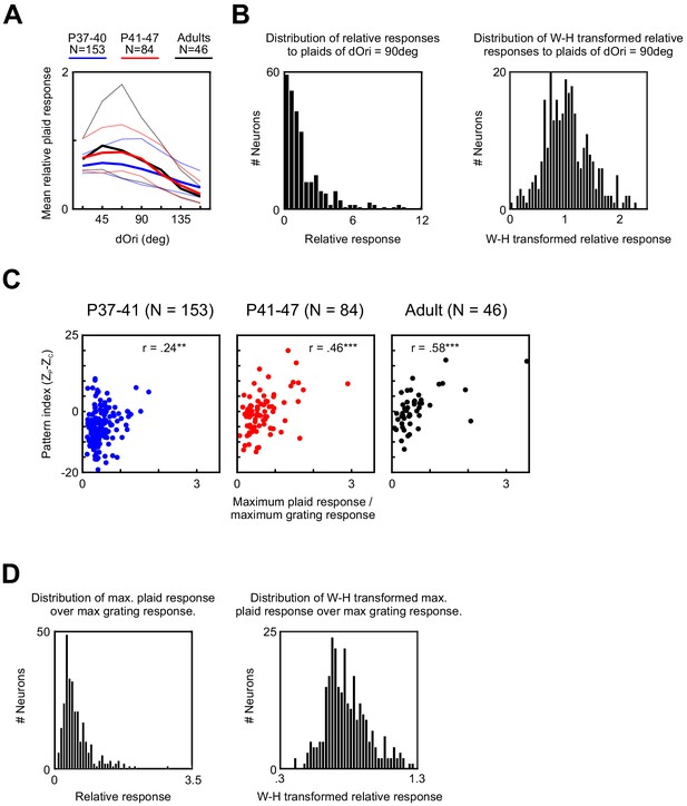
Relative plaid responses in PSS and the Wilson–Hilferty transformation.

(A) Average relative plaid response in PSS as a function of dOri. For each age group, curves indicate the median (solid line) and upper and lower 25th percentile (dotted lines). (B) Distribution of the relative plaid response, computed as the ratio between the mean response to plaids of dOri = 90 deg and the mean response to gratings. Distribution is shown for all PSS cells before (left) and after (right) applying the Wilson–Hilferty transformation. (C) Ratio between the maximum response to plaids (dOri = 90 deg) and the maximum response to gratings versus pattern index at different ages. Same data as in Figure 4C, but without the Wilson–Hilferty transformation. (D) Distribution of the ratio between the maximum response to plaids (dOri = 90 deg) and the maximum response to grating for all PSS cells before (left) and after (right) applying the Wilson–Hilferty transformation.

Figure 5 with 1 supplement

Download asset Open asset

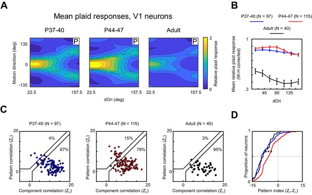
V1 responses to plaids change during PSS motion integration development.

(A) Average 2D profile of responses to plaids in V1 at different ages (computed and plotted as in Figure 4A). (B) Average relative plaid response in V1 as a function of dOri (data shown after Wilson–Hilferty transformation; same format as Figure 4B). Error bars: ± SEM. (C) Pattern versus component correlations for V1 neurons in different age groups (same format as Figure 2C). (D) Cumulative distribution plots for V1 pattern indices at different ages. Same N and color scheme as (C).

Figure 5—source data 1 Neuron-by-neuron metrics for Figure 5 and Figure 5—figure supplement 1.: https://cdn.elifesciences.org/articles/59798/elife-59798-fig5-data1-v2.xlsx
Download elife-59798-fig5-data1-v2.xlsx

Figure 5—figure supplement 1

Download asset Open asset

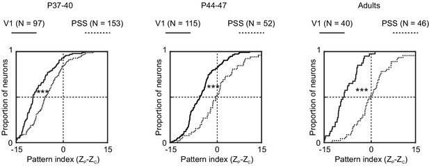
Motion integration levels in V1 are lower than those in PSS across development.

Cumulative distribution of pattern indices for cells recorded in V1 (solid line) and PSS (dashed line) at different ages. Left: P37–40. Middle: P44–47. Right: Adults.

***p<0.001.

Figure 6

Download asset Open asset

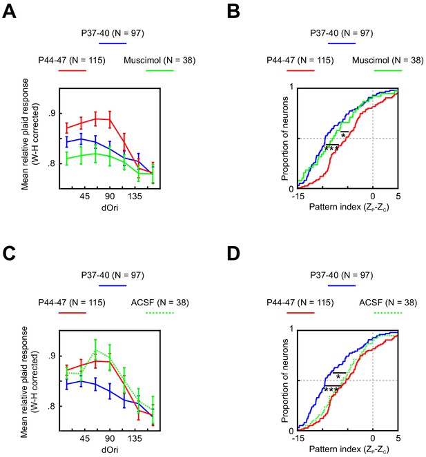
Changes in V1 responses at P44–47 depend on feedback from PSS.

(A) Average relative plaid response in V1 at P37–40 (same data as Figure 5B), P44–47 (same data as Figure 5B), and P44–47 with muscimol inactivation of PSS. Error bars indicate ± SEM. Data are shown after a Wilson–Hilferty transformation. For statistical analysis of data across age groups, see Table 1. (B) Cumulative distribution of V1 pattern indices at P37–40 (same data as Figure 5D), P44–47 (same data as Figure 5D), and P44–47 with muscimol inactivation of PSS. For statistical analysis of data across age groups, see Table 1. *p<0.05. ***p<0.001. (**C, D**) Same plots as (A, B) but after a control injection of ACSF into PSS. Note that the ACSF group included one animal aged P48, making the age range for this group P44–48.

Figure 6—source data 1 Neuron-by-neuron metrics for Figure 6.: https://cdn.elifesciences.org/articles/59798/elife-59798-fig6-data1-v2.xlsx
Download elife-59798-fig6-data1-v2.xlsx

Figure 7

Download asset Open asset

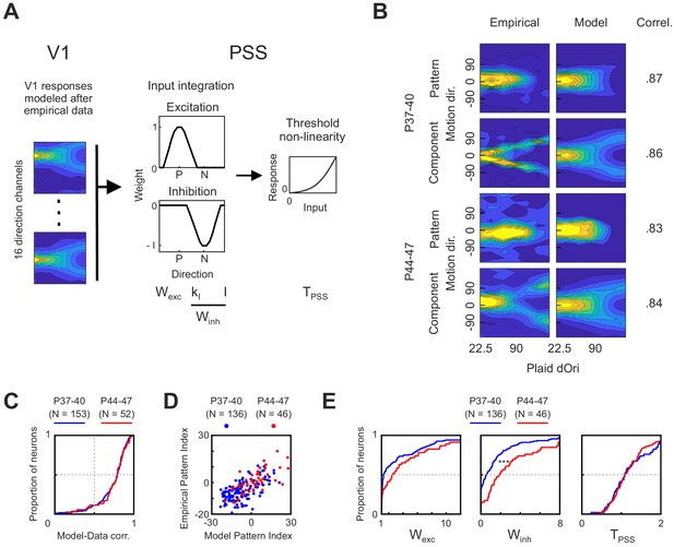
A computational model of the ferret motion pathway for testing mechanisms behind motion integration development.

(A) Diagram of the model used to explain PSS plaid responses across development. The first stage was composed of 16 V1 direction selective cells whose responses were modeled after empirical V1 data from different age groups. Responses from the V1 stage were then integrated in PSS using a combination of an excitatory and an inhibitory weight function (P, preferred direction; N, null direction). Finally, an exponential non-linearity was applied to the PSS responses. The model had four variables, which are listed below the stage to which they belong. For analysis of model results the two variables controlling inhibition (K_I and I) where combined into a single metric (W_inh, see Materials and methods). (B) Examples of empirical PSS responses to plaids (left column) and corresponding model PSS responses (right column) after optimizing model parameters to maximize the likelihood of the empirical data for each neuron. Examples show one pattern and one component cell from animals before (P37–40) and after (P44–47) development of motion integration in PSS. Numbers to the right of response profiles indicate correlation between model and empirical responses. (C) Distribution of correlation coefficients between model and empirical responses for each PSS neuron in the two age groups. Results from neurons with model-data correlation below 0.5i were excluded from further analyses. (D) PSS pattern index for every neuron, computed using empirical data or model data for the neuron, for both age groups. (E) Cumulative distribution of all model variables after fitting the model to data from kits before (P37–40) and after (P44–47) the development of motion integration. ***p<0.001.

Figure 7—source data 1 Neuron-by-neuron metrics for Figure 7.: https://cdn.elifesciences.org/articles/59798/elife-59798-fig7-data1-v2.xlsx
Download elife-59798-fig7-data1-v2.xlsx

Figure 8 with 1 supplement

Download asset Open asset

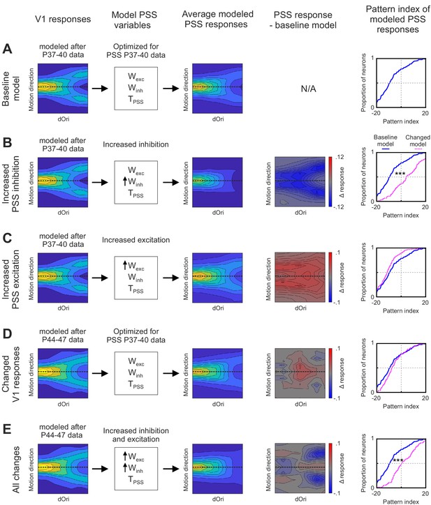
Effects of changes in V1 and PSS mechanisms on PSS plaid responses.

Summary of different instantiations of the motion pathway model. (A) Baseline model. (B) Model with increased PSS inhibition. (C) Model with increased PSS excitation . (D) Model with V1 responses set to reflect those measured at P44–47. (E) Model combining all changes described for (B), (C), and (D). For each model instantiation, the columns (from left to right) contain the following information: Colum 1: V1 plaid responses used for the model’s first stage. Dashed line indicates the preferred motion direction. Column 2: State of PSS parameters for motion integration (W_exc), inhibition (W_inh), and threshold non-linearity (T_PSS) relative to the baseline model (determined by fitting the model to data from P37–40). No arrow indicates values were unchanged relative to the baseline model, upwards arrow indicate an increase in the parameter. Column 3: Average plaid responses of model PSS neurons. Dashed line indicates the preferred motion direction. Column 4: Difference between average plaid responses of model PSS neurons in a model instantiation and the average response in the baseline model. Column 5: Cumulative distribution of pattern indices of model PSS neurons for the new model instantiation (dashed pink line) and baseline model (solid blue line). ***p<0.001.

Figure 8—source data 1 Neuron-by-neuron metrics for Figure 8 and Figure 8—figure supplement 1.: https://cdn.elifesciences.org/articles/59798/elife-59798-fig8-data1-v2.xlsx
Download elife-59798-fig8-data1-v2.xlsx

Figure 8—figure supplement 1

Download asset Open asset

Changes in PSS inhibition parameters with development and model parameter settings for the different model instantiations.

(A) Changes in the two model variables that control PSS inhibition (K_I, left; I, right) with development, determined by fitting the model to data from the two age groups, with the V1 stage set to the appropriate age as well. While there are significant changes in I, changes in K_I are not significant. ***p<0.001. (B) Cumulative distribution plots of W_inh (left) and W_exc (right) in the two age groups and for the model instantiations used for Figure 8B,C and E. ***p<0.001.

Tables

Table 1

Extended information for all statistical analyses.

Figure	Experimental groups	Metric or variable	Test	p-value	Other stats
Figure 1 Sup 1	P37 vs adult	Direction selectivity index	Welch’s t-test	0.86	d’ = 0.04

Figure 2A	P37–40 vs P41–47	Animal median pattern index	Welch’s t-test	0.002	d’ = 1.1
Figure 2A	P37–40 vs adult	Animal median pattern index	Welch’s t-test	0.001	d’ = 1.4
Figure 2A	P41–47 vs adult	Animal median pattern index	Welch’s t-test	0.59	d’ = 0.23
Figure 2A	P37–40 vs P41–47	Animal median pattern index	Resample test	<0.001
Figure 2A	P37–40 vs adult	Animal median pattern index	Resample test	<0.001

Figure 2B	P37–40 vs P41–47	Pattern index. Multiple dOri	Welch’s t-test	<0.001	d’ = 0.74
Figure 2B	P37–40 vs adult	Pattern index. Multiple dOri	Welch’s t-test	<0.001	d’ = 0.96
Figure 2B	P41–47 vs adult	Pattern index. Multiple dOri	Welch’s t-test	0.3	d’ = 0.19
Figure 2B	P37–40 vs P41–47	Pattern index. Multiple dOri	Resample test	<0.001
Figure 2B	P37–40 vs adult	Pattern index. Multiple dOri	Resample test	<0.001

Figure 2 Sup 1	P37–40 vs P41–47	Z_p. Multiple dOri	Welch’s t-test	<0.001	d’ = 0.74
Figure 2 Sup 1	P37–40 vs adult	Z_p. Multiple dOri	Welch’s t-test	<0.001	d’ = 1.0
Figure 2 Sup 1	P41–47 vs adult	Z_p. Multiple dOri	Welch’s t-test	0.24	d’ = 0.22
Figure 2 Sup 1	P37–40 vs P41–47	Z_p. Multiple dOri	Resample test	<0.001
Figure 2 Sup 1	P37–40 vs adult	Z_p. Multiple dOri	Resample test	<0.001

Figure 2 Sup 1	P37–40 vs P41–47	Z_c. Multiple dOri	Welch’s t-test	<0.001	d’ = 0.61
Figure 2 Sup 1	P37–40 vs adult	Z_c. Multiple dOri	Welch’s t-test	<0.001	d’ = 0.73
Figure 2 Sup 1	P41–47 vs adult	Z_c. Multiple dOri	Welch’s t-test	0.58	d’ = 0.10
Figure 2 Sup 1	P37–40 vs P41–47	Z_c. Multiple dOri	Resample test	<0.001
Figure 2 Sup 1	P37–40 vs adult	Z_c. Multiple dOri	Resample test	<0.001

Figure 2E	P37–40 vs P41–47	Pattern index. dOri 135 deg	Welch’s t-test	<0.001	d’ = 1.3
Figure 2E	P37–40 vs adult	Pattern index. dOri 135 deg	Welch’s t-test	<0.001	d’ = 0.94
Figure 2E	P41–47 vs adult	Pattern index. dOri 135 deg	Welch’s t-test	0.43	d’ = 0.21
Figure 2E	P37–40 vs P41–47	Pattern index. dOri 135 deg	Resample test	<0.001
Figure 2E	P37–40 vs adult	Pattern index. dOri 135 deg	Resample test	0.005

Figure 3A	V4 vs V5	Median pattern index	Welch’s t-test	0.005	d’ = 1.8
Figure 3A	V4 vs V6	Median pattern index	Welch’s t-test	0.02	d’ = 1.3
Figure 3A	V5 vs V6	Median pattern index	Welch’s t-test	0.89	d’ = 0.07
Figure 3C	V4 vs V5–6	Pattern index	Welch’s t-test	0.01	d’ = 0.5
Figure 3C	V4 vs V5–6	Pattern index	Resample test	0.03
Figure 3D	V4 vs V5–6	Z_p	Welch’s t-test	0.03	d’ = 0.42
Figure 3D	V4 vs V5–6	Z_p	Resample test	0.04
Figure 3D	V4 vs V5–6	Z_c	Welch’s t-test	0.02	d’ = 0.52
Figure 3D	V4 vs V5–6	Z_c	Resample test	0.03

Figure 4B	P37–40 vs P41–47	Relative plaid responses. Wilson–Hilferty transform	ANOVA. Var: age.	0.80	F = 0.07
Figure 4B	P37–40 vs P41–47	Relative plaid responses. Wilson–Hilferty transform.	ANOVA. Var: dOri	<0.001	F = 60
Figure 4B	P37–40 vs P41–47	Relative plaid responses. Wilson–Hilferty transform.	ANOVA. Var: interaction	0.006	F = 3
Figure 4B	P37–40 vs adult	Relative plaid responses. Wilson–Hilferty transform.	ANOVA. Var: age.	0.08	F = 3.1
Figure 4B	P37–40 vs adult	Relative plaid responses. Wilson–Hilferty transform.	ANOVA. Var: dOri	<0.001	F = 44
Figure 4B	P37–40 vs adult	Relative plaid responses. Wilson–Hilferty transform.	ANOVA. Var: interaction	<0.001	F = 4.2
Figure 4B	P41–47 vs adult	Relative plaid responses. Wilson–Hilferty transform.	ANOVA. Var: age.	0.16	F = 2
Figure 4B	P41–47 vs adult	Relative plaid responses. Wilson–Hilferty transform.	ANOVA. Var: dOri	<0.001	F = 51
Figure 4B	P41–47 vs adult	Relative plaid responses. Wilson–Hilferty transform.	ANOVA. Var: interaction	0.64	F = 0.7

Figure 4B	P37–40 vs P41–47	Relative plaid responses. dOri: 45 deg. Wilson–Hilferty transform.	Welch’s t-test	0.16	d’=0.19
Figure 4B	P37–40 vs adult	Relative plaid responses. dOri: 45 deg. Wilson–Hilferty transform.	Welch’s t-test	0.005	d’ = 0.58
Figure 4B	P41–47 vs adult	Relative plaid responses. dOri: 45 deg. Wilson-Hilferty transform.	Welch’s t-test	0.06	d’ = 0.39
Figure 4B	P37–40 vs adult	Relative plaid responses. dOri: 45 deg. Wilson–Hilferty transform.	Resample test	<0.001

Figure 4B	P37–40 vs P41–47	Relative plaid responses. dOri: 157 deg. Wilson–Hilferty transform.	Welch’s t-test	0.02	0.32
Figure 4B	P37–40 vs adult	Relative plaid responses. dOri: 157 deg. Wilson–Hilferty transform.	Welch’s t-test	0.01	0.42
Figure 4B	P41–47 vs adult	Relative plaid responses. dOri: 157 deg. Wilson–Hilferty transform.	Welch’s t-test	0.53	0.12
Figure 4B	P37–40 vs P41–47	Relative plaid responses. dOri: 157 deg. Wilson–Hilferty transform.	Resample test	0.002
Figure 4B	P37–40 vs adult	Relative plaid responses. dOri: 157 deg. Wilson–Hilferty transform.	Resample test	<0.001

Figure 4C	P37–40	Pattern index vs relative plaid response. Wilson–Hilferty transform	Pearson correlation	0.009	r = 0.21
Figure 4C	P41–47	Pattern index vs relative plaid response. Wilson–Hilferty transform.	Pearson correlation	<0.001	r = 0.46
Figure 4C	Adult	Pattern index vs relative plaid response. Wilson–Hilferty transform	Pearson correlation	<0.001	r = 0.60
Figure 4C	P47–40 vs adult	Pattern index vs relative plaid response. Wilson–Hilferty transform	Correlation difference	0.02	z = 2.06
Figure 4C	P47–40 vs P41–47	Pattern index vs relative plaid response. Wilson–Hilferty transform	Correlation difference	0.003	z = 2.77

Figure 4 Sup 1C	P37–40	Pattern index vs relative plaid response.	Pearson correlation	0.003	r = 0.24
Figure 4 Sup 1C	P41–47	Pattern index vs relative plaid response.	Pearson correlation	<0.001	r = 0.46
Figure 4 Sup 1C	Adult	Pattern index vs relative plaid response.	Pearson correlation	<0.001	r = 0.58

Figure 5B	P37–40 vs P44–47	Relative plaid responses. Wilson–Hilferty transform	ANOVA. Var: age.	0.001	F = 11
Figure 5B	P37–40 vs P44–47	Relative plaid responses. Wilson–Hilferty transform.	ANOVA. Var: dOri	<0.001	F = 11
Figure 5B	P37–40 vs P44–47	Relative plaid responses. Wilson–Hilferty transform.	ANOVA. Var: interaction	0.26	F = 1.3
Figure 5B	P37–40 vs adult	Relative plaid responses. Wilson–Hilferty transform.	ANOVA. Var: age.	<0.001	F = 82
Figure 5B	P37–40 vs adult	Relative plaid responses. Wilson–Hilferty transform.	ANOVA. Var: dOri	<0.001	F = 6.8
Figure 5B	P37–40 vs adult	Relative plaid responses. Wilson-Hilferty transform.	ANOVA. Var: interaction	0.10	F = 1.8
Figure 5B	P44–47 vs adult	Relative plaid responses. Wilson–Hilferty transform.	ANOVA. Var: age	<0.001	F = 100
Figure 5B	P44–47 vs adult	Relative plaid responses. Wilson–Hilferty transform.	ANOVA. Var: dOri	<0.001	F = 7
Figure 5B	P44–47 vs adult	Relative plaid responses. Wilson–Hilferty transform.	ANOVA. Var: interaction	0.03	F = 2.3

Figure 5D	P37–40 vs P44–47	Pattern index. dOri 135 deg	Welch’s t-test	<0.001	d’ = 0.61
Figure 5D	P37–40 vs adult	Pattern index. dOri 135 deg	Welch’s t-test	0.94	d’ = 0.01
Figure 5D	P44–47 vs adult	Pattern index. dOri 135 deg	Welch’s t-test	<0.001	d’ = 0.64
Figure 5D	P44–47 vs adult	Pattern index. dOri 135 deg	Resample test	<0.001

Figure 6A	P44–47 vs muscimol	Relative plaid responses. Wilson–Hilferty transform	ANOVA. Var: Muscimol.	<0.001	F = 17
Figure 6A	P44–47 vs muscimol	Relative plaid responses. Wilson–Hilferty transform.	ANOVA. Var: dOri	<0.001	F = 4.5
Figure 6A	P44–47 vs muscimol	Relative plaid responses. Wilson–Hilferty transform.	ANOVA. Var: interaction	0.44	F = 0.97
Figure 6C	P44-47 vs ACSF	Relative plaid responses. Wilson–Hilferty transform.	ANOVA. Var: ACSF.	0.56	F = 0.32
Figure 6C	P44–47 vs ACSF	Relative plaid responses. Wilson–Hilferty transform.	ANOVA. Var: dOri	<0.001	F = 8.3
Figure 6C	P44–47 vs ACSF	Relative plaid responses. Wilson–Hilferty transform.	ANOVA. Var: interaction	0.98	F = 0.20
Figure 6A	P37–40 vs muscimol	Relative plaid responses. Wilson–Hilferty transform	ANOVA. Var: Muscimol.	0.04	F = 4.3
Figure 6A	P37–40 vs muscimol	Relative plaid responses. Wilson–Hilferty transform.	ANOVA. Var: dOri	0.007	F = 3.0
Figure 6A	P37–40 vs muscimol	Relative plaid responses. Wilson–Hilferty transform.	ANOVA. Var: interaction	0.94	F = 0.29
Figure 6C	P37–40 vs ACSF	Relative plaid responses. Wilson–Hilferty transform.	ANOVA. Var: ACSF.	<0.001	F = 12
Figure 6C	P37–40 vs ACSF	Relative plaid responses. Wilson–Hilferty transform.	ANOVA. Var: dOri	<0.001	F = 6.6
Figure 6C	P37–40 vs ACSF	Relative plaid responses. Wilson–Hilferty transform.	ANOVA. Var: interaction	0.42	F = 1

Figure 6B	P44–47 vs muscimol	Pattern index	Welch’s t-test	0.01	d’ = 0.52
Figure 6D	P44–47 vs ACSF	Pattern index	Welch’s t-test	0.4	d’ = 0.15
Figure 6B	P37–41 vs muscimol	Pattern index	Welch’s t-test	0.71	d’ = 0.07
Figure 6D	P37–41 vs ACSF	Pattern index	Welch’s t-test	0.02	d’ = 0.46
Figure 6B	P44–47 vs muscimol	Pattern index	Resample test	0.02
Figure 6B	P37–41 vs ACSF	Pattern index	Resample test	0.01

Figure 7C	P37–40 vs P44–47	Model-data correlation	Rank-sum test	0.14
Figure 7E	P37–40 vs P44–47	Model excitation (W_exc)	Rank-sum test	0.06
Figure 7E	P37–40 vs P44–47	Model inhibition (W_inh)	Rank-sum test	<0.001
Figure 7E	P37–40 vs P44–47	Model PSS threshold (T_PSS)	Rank-sum test	0.96
Figure 7E	P37–40 vs P44–47	Model inhibition (W_inh)	Resample test	<0.001

Table 2

Number of animals and neurons for all experiments.

Figures	Experiment/analysis	Experimental group	Animals	Neurons
1 Sup 1	Analysis of direction selectivity using gratings.	PSS. P37.	3	37
1 Sup 1	Analysis of direction selectivity using gratings.	PSS. Adult.	10	68
1, 2, and 4	Analysis of pattern index and dOri tuning using responses to plaids of different dOri values.	PSS. P37–40.	27	153
1, 2, and 4	Analysis of pattern index and dOri tuning using responses to plaids of different dOri values.	PSS. P41–47.	13	84
1, 2, and 4	Analysis of pattern index and dOri tuning using responses to plaids of different dOri values.	PSS. Adult.	9	46
3	Analysis of pattern index and dOri tuning using responses to plaids of different dOri values.	PSS. V4.	4	33
3	Analysis of pattern index and dOri tuning using responses to plaids of different dOri values.	PSS. V5.	8	34
3	Analysis of pattern index and dOri tuning using responses to plaids of different dOri values.	PSS. P37.	6	36
3	Analysis of pattern index and dOri tuning using responses to plaids of different dOri values.	PSS. P40.	8	38
2 Sup 1	Analysis of pattern index using responses to plaids of dOri 135 deg.	PSS. P37–40.	6	12
2 Sup 1	Analysis of pattern index using responses to plaids of dOri 135 deg.	PSS. P41–47.	5	23
2 Sup 1	Analysis of pattern index using responses to plaids of dOri 135 deg.	PSS. Adult.	7	35
5, 6	Analysis of pattern index and dOri tuning using responses to plaids of different dOri values.	V1. P37–40.	16	97
5, 6	Analysis of pattern index and dOri tuning using responses to plaids of different dOri values.	V1. P41-47.	14	115
5	Analysis of pattern index and dOri tuning using responses to plaids of different dOri values.	V1. Adult.	9	40
6	Analysis of pattern index and dOri tuning using responses to plaids of different dOri values.	Muscimol	5	38
6	Analysis of pattern index and dOri tuning using responses to plaids of different dOri values.	ACSF	3	38
7, 8	Analysis of model MLE fits.	PSS. P37-40.	25	136
7	Analysis of model MLE fits.	PSS. P44-47.	8	46