Development of visual motion integration involves coordination of multiple cortical stages

Version of Record

Accepted for publication after peer review and revision.

Download
Cite
Share
CommentOpen annotations (there are currently 0 annotations on this page).

660 views

Version of Record updated: March 24, 2021 (This version)
Version of Record published: March 22, 2021 (Go to version)
Accepted: March 8, 2021
Received: June 8, 2020

1. Of interest
Balancing true and false detection of intermittent sensory targets by adjusting the inputs to the evidence accumulation process

Anna C Geuzebroek, Hannah Craddock ... Simon P Kelly

Research Article Oct 3, 2023
Further reading

Abstract
Introduction
Results
Discussion
Materials and methods
Data availability
References
Decision letter
Author response
Article and author information
Metrics

Abstract

A central feature of cortical function is hierarchical processing of information. Little is currently known about how cortical processing cascades develop. Here, we investigate the joint development of two nodes of the ferret’s visual motion pathway, primary visual cortex (V1), and higher-level area PSS. In adult animals, motion processing transitions from local to global computations between these areas. We now show that PSS global motion signals emerge a week after the development of V1 and PSS direction selectivity. Crucially, V1 responses to more complex motion stimuli change in parallel, in a manner consistent with supporting increased PSS motion integration. At the same time, these V1 responses depend on feedback from PSS. Our findings suggest that development does not just proceed in parallel in different visual areas, it is coordinated across network nodes. This has important implications for understanding how visual experience and developmental disorders can influence the developing visual system.

Introduction

Information processing in the brain involves a chain of transformations across areas, linked via feedforward and feedback loops. Little is currently known about how this interconnected network of areas develops. Yet, without a precise determination of at least the relative developmental time courses of different areas, models for cortical development remain lacking, as does our understanding of whether and how interactions between areas might shape the emerging network. The motion pathway in visual cortex provides a unique opportunity to address these questions: Its central nodes are well established in the primate, as are key pathway functions (Born and Bradley, 2005; Orban, 2008). Accordingly, there are well-characterized stimulus sets for probing these functions and a range of computational models for the motion pathway (Baker and Bair, 2016; Beck and Neumann, 2011; Rust et al., 2006; Simoncelli and Heeger, 1998; Zaharia et al., 2019). This holds true in particular for motion integration: Between primary visual cortex (V1) and area MT, the next motion pathway stage, the encoding of motion information transitions from extracting local edge signals to computing global motion signals (Born and Bradley, 2005; Orban, 2008; Movshon et al., 1985). Typically, this is demonstrated using drifting plaids, constructed from two component gratings moving in different directions (Movshon et al., 1985). Perceptually, plaids appear to move in a third, intermediate (pattern) direction (Adelson and Movshon, 1982; Stoner et al., 1990). By probing whether neural responses are consistent with the individual component directions or the integrated pattern direction, the degree of motion integration in a neuron or area can be assessed. Applied to V1, these stimuli reveal mostly component-driven responses (Movshon et al., 1985). In primate MT, on the other hand, a quarter of the population responds to the pattern direction, indicative of an increased degree of motion integration as necessary for global motion computations (Movshon et al., 1985). Finally, a number of models have been developed to capture the transformation of motion signals between V1 and MT (Baker and Bair, 2016; Beck and Neumann, 2011; Rust et al., 2006; Simoncelli and Heeger, 1998; Zaharia et al., 2019). Thus, the stage is set – both from an experimental and computational perspective – for using the motion pathway, and specifically motion integration, to investigate the joint development of interconnected cortical areas.

To date, the visual motion pathway has been most thoroughly investigated in adult non-human primates. Much less is known about its development (Chino et al., 1997; Kiorpes and Movshon, 2014). We have recently demonstrated that area PSS in ferret visual cortex shares many similarities with primate MT (Lempel and Nielsen, 2019). Crucially, the same transition from local to global motion processing occurs between ferret V1 and PSS as between primate V1 and MT. At the same time, the ferret’s early parturition (Sharma and Sur, 2014) allows easy access to the development of these stages. Here, we leveraged the strength of the ferret as a developmental animal model, combined with our previous research on PSS, to probe the development of motion integration in the motion pathway. Using single-cell recordings, we found that PSS motion integration develops after postnatal day (P) 40, during the second week after eye opening, and after the development of direction selectivity. Maturation of motion integration was reflected not only in an increasing prevalence of pattern responses, but also in how responses depended on the exact plaid configuration. We also provide evidence that visual experience likely plays a role in the development of this process.

Intriguingly, we additionally observed developmental changes in V1 responses to plaids, highlighting the need to consider multiple pathway stages simultaneously during development. V1 development included a temporary increase in motion integration and plaid response strength between P44 and P47. Inactivation of PSS demonstrated that both of these changes depended on feedback from PSS. At the same time, we expect that changes in V1 responses are likely to propagate to PSS. To test how these V1 changes might complement PSS changes during motion integration development, we implemented a two-stage model of the ferret’s motion pathway. The model was then used to identify the relative contributions of V1 and PSS development to the increase in PSS pattern responses after P40. This modeling exercise suggested development of strong inhibition between preferred and null direction, internal to PSS, as an important contributor to increased motion integration. At the same time, the temporary changes in V1 plaid responses complemented PSS-internal changes to overcome possibly detrimental consequences of the increased inhibition levels, namely overall reductions in PSS pattern responses. In summary, our results reveal that development of the motion pathway involves coordination between multiple network nodes in a highly dynamic fashion.

Results

Developmental timeline of PSS motion integration

Using coherent plaids, we have previously demonstrated signatures of motion integration in PSS of adult ferrets (Figure 1A). Specifically, a group of PSS neurons responds to the pattern direction of the plaids (so called ‘pattern neurons’), rather than the motion of the individual components (as would be the case for so called ‘component neurons’). Here, we first aimed to establish the developmental timeline for PSS pattern responses. To this end, we used tetrodes or multi-channel silicon probes to record PSS responses in anesthetized ferrets at various ages. Previous research in primates suggests that motion integration develops after maturation of direction selectivity (Chino et al., 1997; Kiorpes and Movshon, 2014). In addition, a minimal level of direction selectivity is required for a meaningful analysis of responses to plaids. We therefore restricted our experiments to an age range after V1 direction selectivity development, which in ferrets occurs around P37 (ferrets open their eyes at about P30). Our data confirm that PSS direction selectivity is also mature at this age (see Figure 1—figure supplement 1).

Figure 1 with 1 supplement see all

Download asset Open asset

Pattern and component cells are found in PSS across all ages tested.

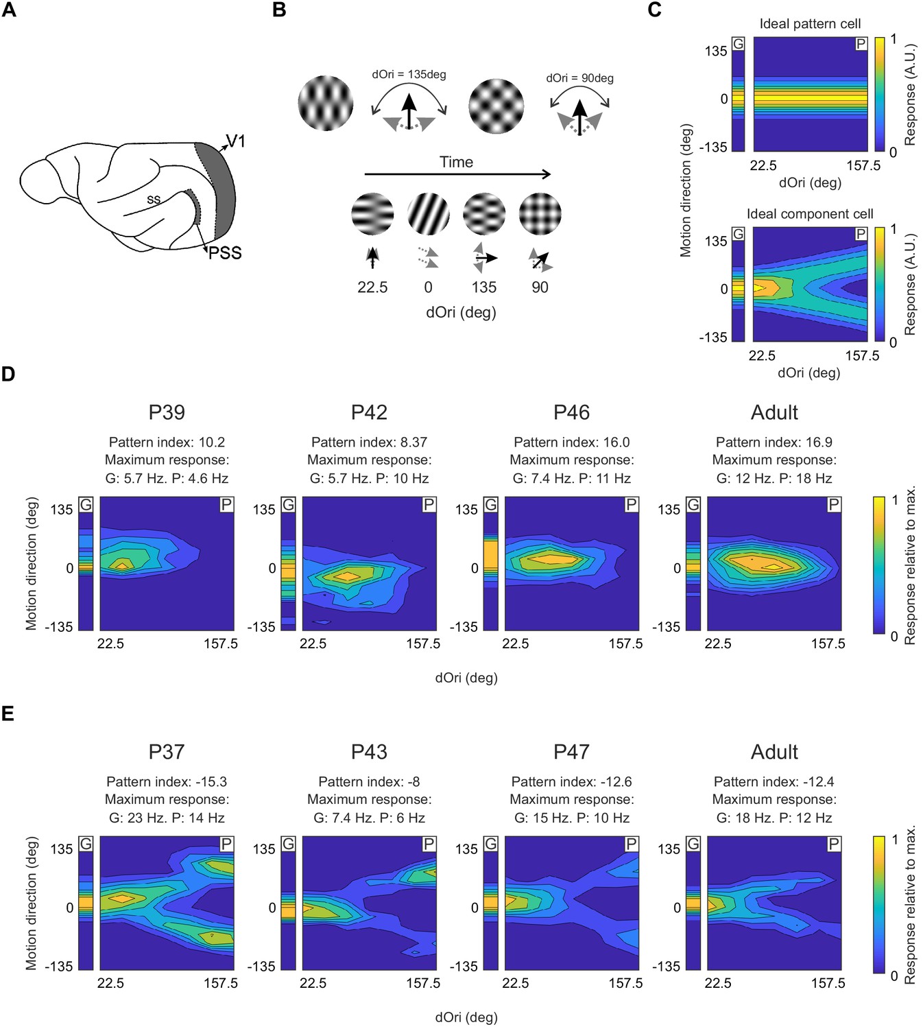
(A) Sagittal view of the ferret brain indicating the location of PSS and V1 (ss: suprasylvian sulcus). (B) Top: Plaid stimuli with different angles between the component directions (dOri). Bottom: Illustration of the streaming stimulus paradigm: Plaids of different dOri values and directions were presented along with gratings moving in different directions (see Materials and methods). (C) Simulated responses of an ideal pattern (top) and component cell (bottom) to gratings and plaids. In this and the following figures, the small contour plot for each cell (labeled ‘G’) represents the responses to gratings only. The large 2D contour plot (labeled ‘P’) summarizes responses to all plaids as a function of dOri and direction. In both plots, direction is relative to the cell’s preferred grating direction. For ‘G’, direction refers to the grating direction; for ‘P’, direction refers to the pattern direction (i.e. the perceived direction of the plaid). ‘G’ and ‘P’ are independently normalized by their respective maximum to help with visualization of the tuning properties. An ideal pattern cell would respond maximally to plaid stimuli moving in its preferred direction. An ideal component cell would respond maximally whenever one plaid component moves in the preferred direction, resulting in a response profile with a characteristic ‘V’-shape. For the ideal cells, resposes were scaled so that the area under the direction curve remained constant across dOri values. As a consequence, the responses for the ideal component cell change with dOri (because different number of directions evoke strong responses). All other dOri dependencies were ignored in this illustration. (D) Responses of example PSS neurons classified as pattern cells (see Materials and methods for classification procedure) in ferrets of different ages. For each neuron, we list the pattern index, as well as the maximum response rate evoked by gratings (G) and plaids (P) (otherwise same format as in (C)). (E) Responses of example PSS component cells in ferrets of different age (same format as (D)).

PSS motion integration was assessed at different ages by probing neurons with plaids and gratings. Since plaids are constructed from two component gratings moving in different directions, each plaid can be described by two parameters (Figure 1B) – the difference in direction between the two components (dOri) and the resulting plaid direction (which bisects the two component directions). Importantly, the perception of a coherently moving plaid is maintained over a large range of dOri values (Adelson and Movshon, 1982). To efficiently sample a large number of dOri values and plaid directions, we presented stimuli in a streaming stimulus paradigm, in which stimuli were shown in rapid succession (stimulus update rate: 3 Hz; Figure 1B). We have previously shown that the results of this approach generally agree with those based on showing single stimuli more slowly, but that the sampling of a larger stimulus space noticeably improves the discriminability of pattern and component responses, in addition to generating results that are independent of a particular dOri choice (see Rust et al., 2006; Smith et al., 2005 for a similar presentation method).

For every neuron probed with the streaming stimulus paradigm, we then determined its capacity to integrate local motion signals (see Lempel and Nielsen, 2019 and Materials and methods for details). Briefly, for every neuron, we generated two predictions from the measured stimulus responses, one for pattern and one for component responses. Each prediction summarized tuning as a two-dimensional (2D) function of both the (integrated) plaid direction and dOri. Since coherent plaid motion is perceived independent of dOri, the pattern prediction assumed that the tuning peak would always occur for plaids moving in the preferred direction, regardless of dOri value (but allowing changes in peak height in a dOri-dependent fashion). Consequently, tuning profiles for pattern predictions had a single ridge along the preferred direction (Figure 1C, top). The component prediction, on the other hand, assumed that the individual component directions determined responses, not the integrated plaid direction. For each dOri, the strongest responses therefore should occur whenever one of the components moved in the preferred direction, resulting in a characteristic ‘V’-shape in the chosen 2D tuning plot format (Figure 1C, bottom). As for the pattern prediction, dOri-dependent changes in maximum rates were included in the component prediction. We then compared the two predictions to the measured tuning profile of each neuron by computing Z-corrected partial correlations, resulting in a pattern correlation (Z_P) and a component correlation (Z_C). We also computed a pattern index for every neuron as Z_P–Z_C. Based on established criteria (Smith et al., 2005), neurons were classified as pattern neurons if Z_P was significantly higher than Z_C (using p<0.1); component neurons met the opposite criterion (see Figure 2C and Materials and methods for precise definitions of category boundaries).

Figure 2 with 1 supplement see all

Download asset Open asset

Motion integration in PSS matures around P41.

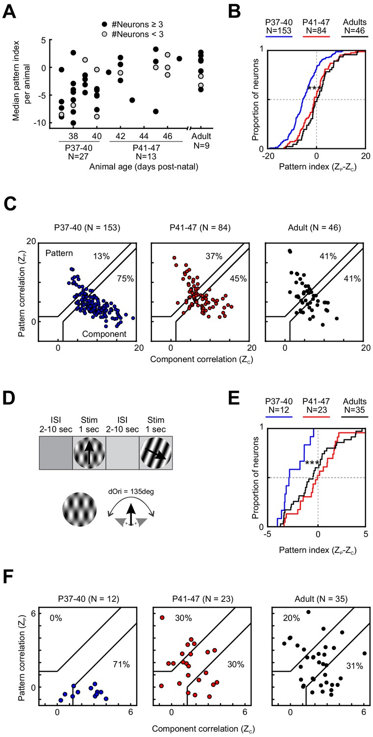
(A) Median PSS pattern index for each animal included in the study, plotted as a function of age. Gray dots represent animals that yielded one to two neurons, black dots represent animals with data for at least three neurons. (B) Cumulative distributions for pattern indices in different age groups. For further information on statistical tests for this and all following plots, see Table 1. ***p<0.001. (C) Pattern versus component correlations for PSS neurons in animals from different age groups. For each neuron, Z_P is plotted against Z_C. Black lines indicate the category boundaries used to classify cells into pattern, unclassified, and component cells. Percentages indicate the portion of neurons falling into the component and pattern categories. (D) Top: Illustration of the classic stimulus presentation paradigm, in which stimuli were presented for 1 s, and stimulus presentations were interleaved by 2–10 s of inter-stimulus interval. Bottom: Example plaid stimulus with 135 degrees of difference between the component directions. (E) Same as (B), but for pattern indices computed from responses to plaids presented in the classic stimulus paradigm as shown in (D). ***p<0.001. (F) Same as (C), but for pattern and component correlations computed based on the classic stimulus paradigm as shown in (D).

Figure 2—source data 1 Neuron-by-neuron metrics for Figure 2 and Figure 2—figure supplement 1.: https://cdn.elifesciences.org/articles/59798/elife-59798-fig2-data1-v2.xlsx
Download elife-59798-fig2-data1-v2.xlsx

Across all ages tested (P37–13 months), we were able to observe pattern and component cells in PSS (Figure 1D,E). Nonetheless, the degree of PSS motion integration underwent pronounced changes with age. As a first step in assessing the time course of motion integration development, we computed the median pattern index for every animal. Figure 2A shows these medians as a function of age (Note that for some animals less than three neurons were recorded. We included these animals for completeness but indicate the corresponding data points in Figure 2A.) While this plot confirmed that a range of pattern indices could be observed at every age, it also showed that the lowest median pattern indices generally occurred in animals before P41. After P41, the range of median pattern indices across animals of the same age was generally similar to that of adults. We therefore divided all developmental data into two groups, P37–40 and P41–47. A third group consisted of adult animals (age range P100–448). As expected, the per-animal pattern indices in the P37–40 age groups were significantly lower than those of the other two groups (P37–40 vs P41–47: p=0.002; P37–40 vs Adult: p=0.001. See Table 1 for the full test details and all statistical results. All data selection criteria are outlined in the Materials and methods. Uneven sample sizes were considered in the choice of statistical tests and are discussed in Materials and methods as well).

Table 1

Extended information for all statistical analyses.

Figure	Experimental groups	Metric or variable	Test	p-value	Other stats
Figure 1 Sup 1	P37 vs adult	Direction selectivity index	Welch’s t-test	0.86	d’ = 0.04

Figure 2A	P37–40 vs P41–47	Animal median pattern index	Welch’s t-test	0.002	d’ = 1.1
Figure 2A	P37–40 vs adult	Animal median pattern index	Welch’s t-test	0.001	d’ = 1.4
Figure 2A	P41–47 vs adult	Animal median pattern index	Welch’s t-test	0.59	d’ = 0.23
Figure 2A	P37–40 vs P41–47	Animal median pattern index	Resample test	<0.001
Figure 2A	P37–40 vs adult	Animal median pattern index	Resample test	<0.001

Figure 2B	P37–40 vs P41–47	Pattern index. Multiple dOri	Welch’s t-test	<0.001	d’ = 0.74
Figure 2B	P37–40 vs adult	Pattern index. Multiple dOri	Welch’s t-test	<0.001	d’ = 0.96
Figure 2B	P41–47 vs adult	Pattern index. Multiple dOri	Welch’s t-test	0.3	d’ = 0.19
Figure 2B	P37–40 vs P41–47	Pattern index. Multiple dOri	Resample test	<0.001
Figure 2B	P37–40 vs adult	Pattern index. Multiple dOri	Resample test	<0.001

Figure 2 Sup 1	P37–40 vs P41–47	Z_p. Multiple dOri	Welch’s t-test	<0.001	d’ = 0.74
Figure 2 Sup 1	P37–40 vs adult	Z_p. Multiple dOri	Welch’s t-test	<0.001	d’ = 1.0
Figure 2 Sup 1	P41–47 vs adult	Z_p. Multiple dOri	Welch’s t-test	0.24	d’ = 0.22
Figure 2 Sup 1	P37–40 vs P41–47	Z_p. Multiple dOri	Resample test	<0.001
Figure 2 Sup 1	P37–40 vs adult	Z_p. Multiple dOri	Resample test	<0.001

Figure 2 Sup 1	P37–40 vs P41–47	Z_c. Multiple dOri	Welch’s t-test	<0.001	d’ = 0.61
Figure 2 Sup 1	P37–40 vs adult	Z_c. Multiple dOri	Welch’s t-test	<0.001	d’ = 0.73
Figure 2 Sup 1	P41–47 vs adult	Z_c. Multiple dOri	Welch’s t-test	0.58	d’ = 0.10
Figure 2 Sup 1	P37–40 vs P41–47	Z_c. Multiple dOri	Resample test	<0.001
Figure 2 Sup 1	P37–40 vs adult	Z_c. Multiple dOri	Resample test	<0.001

Figure 2E	P37–40 vs P41–47	Pattern index. dOri 135 deg	Welch’s t-test	<0.001	d’ = 1.3
Figure 2E	P37–40 vs adult	Pattern index. dOri 135 deg	Welch’s t-test	<0.001	d’ = 0.94
Figure 2E	P41–47 vs adult	Pattern index. dOri 135 deg	Welch’s t-test	0.43	d’ = 0.21
Figure 2E	P37–40 vs P41–47	Pattern index. dOri 135 deg	Resample test	<0.001
Figure 2E	P37–40 vs adult	Pattern index. dOri 135 deg	Resample test	0.005

Figure 3A	V4 vs V5	Median pattern index	Welch’s t-test	0.005	d’ = 1.8
Figure 3A	V4 vs V6	Median pattern index	Welch’s t-test	0.02	d’ = 1.3
Figure 3A	V5 vs V6	Median pattern index	Welch’s t-test	0.89	d’ = 0.07
Figure 3C	V4 vs V5–6	Pattern index	Welch’s t-test	0.01	d’ = 0.5
Figure 3C	V4 vs V5–6	Pattern index	Resample test	0.03
Figure 3D	V4 vs V5–6	Z_p	Welch’s t-test	0.03	d’ = 0.42
Figure 3D	V4 vs V5–6	Z_p	Resample test	0.04
Figure 3D	V4 vs V5–6	Z_c	Welch’s t-test	0.02	d’ = 0.52
Figure 3D	V4 vs V5–6	Z_c	Resample test	0.03

Figure 4B	P37–40 vs P41–47	Relative plaid responses. Wilson–Hilferty transform	ANOVA. Var: age.	0.80	F = 0.07
Figure 4B	P37–40 vs P41–47	Relative plaid responses. Wilson–Hilferty transform.	ANOVA. Var: dOri	<0.001	F = 60
Figure 4B	P37–40 vs P41–47	Relative plaid responses. Wilson–Hilferty transform.	ANOVA. Var: interaction	0.006	F = 3
Figure 4B	P37–40 vs adult	Relative plaid responses. Wilson–Hilferty transform.	ANOVA. Var: age.	0.08	F = 3.1
Figure 4B	P37–40 vs adult	Relative plaid responses. Wilson–Hilferty transform.	ANOVA. Var: dOri	<0.001	F = 44
Figure 4B	P37–40 vs adult	Relative plaid responses. Wilson–Hilferty transform.	ANOVA. Var: interaction	<0.001	F = 4.2
Figure 4B	P41–47 vs adult	Relative plaid responses. Wilson–Hilferty transform.	ANOVA. Var: age.	0.16	F = 2
Figure 4B	P41–47 vs adult	Relative plaid responses. Wilson–Hilferty transform.	ANOVA. Var: dOri	<0.001	F = 51
Figure 4B	P41–47 vs adult	Relative plaid responses. Wilson–Hilferty transform.	ANOVA. Var: interaction	0.64	F = 0.7

Figure 4B	P37–40 vs P41–47	Relative plaid responses. dOri: 45 deg. Wilson–Hilferty transform.	Welch’s t-test	0.16	d’=0.19
Figure 4B	P37–40 vs adult	Relative plaid responses. dOri: 45 deg. Wilson–Hilferty transform.	Welch’s t-test	0.005	d’ = 0.58
Figure 4B	P41–47 vs adult	Relative plaid responses. dOri: 45 deg. Wilson-Hilferty transform.	Welch’s t-test	0.06	d’ = 0.39
Figure 4B	P37–40 vs adult	Relative plaid responses. dOri: 45 deg. Wilson–Hilferty transform.	Resample test	<0.001

Figure 4B	P37–40 vs P41–47	Relative plaid responses. dOri: 157 deg. Wilson–Hilferty transform.	Welch’s t-test	0.02	0.32
Figure 4B	P37–40 vs adult	Relative plaid responses. dOri: 157 deg. Wilson–Hilferty transform.	Welch’s t-test	0.01	0.42
Figure 4B	P41–47 vs adult	Relative plaid responses. dOri: 157 deg. Wilson–Hilferty transform.	Welch’s t-test	0.53	0.12
Figure 4B	P37–40 vs P41–47	Relative plaid responses. dOri: 157 deg. Wilson–Hilferty transform.	Resample test	0.002
Figure 4B	P37–40 vs adult	Relative plaid responses. dOri: 157 deg. Wilson–Hilferty transform.	Resample test	<0.001

Figure 4C	P37–40	Pattern index vs relative plaid response. Wilson–Hilferty transform	Pearson correlation	0.009	r = 0.21
Figure 4C	P41–47	Pattern index vs relative plaid response. Wilson–Hilferty transform.	Pearson correlation	<0.001	r = 0.46
Figure 4C	Adult	Pattern index vs relative plaid response. Wilson–Hilferty transform	Pearson correlation	<0.001	r = 0.60
Figure 4C	P47–40 vs adult	Pattern index vs relative plaid response. Wilson–Hilferty transform	Correlation difference	0.02	z = 2.06
Figure 4C	P47–40 vs P41–47	Pattern index vs relative plaid response. Wilson–Hilferty transform	Correlation difference	0.003	z = 2.77

Figure 4 Sup 1C	P37–40	Pattern index vs relative plaid response.	Pearson correlation	0.003	r = 0.24
Figure 4 Sup 1C	P41–47	Pattern index vs relative plaid response.	Pearson correlation	<0.001	r = 0.46
Figure 4 Sup 1C	Adult	Pattern index vs relative plaid response.	Pearson correlation	<0.001	r = 0.58

Figure 5B	P37–40 vs P44–47	Relative plaid responses. Wilson–Hilferty transform	ANOVA. Var: age.	0.001	F = 11
Figure 5B	P37–40 vs P44–47	Relative plaid responses. Wilson–Hilferty transform.	ANOVA. Var: dOri	<0.001	F = 11
Figure 5B	P37–40 vs P44–47	Relative plaid responses. Wilson–Hilferty transform.	ANOVA. Var: interaction	0.26	F = 1.3
Figure 5B	P37–40 vs adult	Relative plaid responses. Wilson–Hilferty transform.	ANOVA. Var: age.	<0.001	F = 82
Figure 5B	P37–40 vs adult	Relative plaid responses. Wilson–Hilferty transform.	ANOVA. Var: dOri	<0.001	F = 6.8
Figure 5B	P37–40 vs adult	Relative plaid responses. Wilson-Hilferty transform.	ANOVA. Var: interaction	0.10	F = 1.8
Figure 5B	P44–47 vs adult	Relative plaid responses. Wilson–Hilferty transform.	ANOVA. Var: age	<0.001	F = 100
Figure 5B	P44–47 vs adult	Relative plaid responses. Wilson–Hilferty transform.	ANOVA. Var: dOri	<0.001	F = 7
Figure 5B	P44–47 vs adult	Relative plaid responses. Wilson–Hilferty transform.	ANOVA. Var: interaction	0.03	F = 2.3

Figure 5D	P37–40 vs P44–47	Pattern index. dOri 135 deg	Welch’s t-test	<0.001	d’ = 0.61
Figure 5D	P37–40 vs adult	Pattern index. dOri 135 deg	Welch’s t-test	0.94	d’ = 0.01
Figure 5D	P44–47 vs adult	Pattern index. dOri 135 deg	Welch’s t-test	<0.001	d’ = 0.64
Figure 5D	P44–47 vs adult	Pattern index. dOri 135 deg	Resample test	<0.001

Figure 6A	P44–47 vs muscimol	Relative plaid responses. Wilson–Hilferty transform	ANOVA. Var: Muscimol.	<0.001	F = 17
Figure 6A	P44–47 vs muscimol	Relative plaid responses. Wilson–Hilferty transform.	ANOVA. Var: dOri	<0.001	F = 4.5
Figure 6A	P44–47 vs muscimol	Relative plaid responses. Wilson–Hilferty transform.	ANOVA. Var: interaction	0.44	F = 0.97
Figure 6C	P44-47 vs ACSF	Relative plaid responses. Wilson–Hilferty transform.	ANOVA. Var: ACSF.	0.56	F = 0.32
Figure 6C	P44–47 vs ACSF	Relative plaid responses. Wilson–Hilferty transform.	ANOVA. Var: dOri	<0.001	F = 8.3
Figure 6C	P44–47 vs ACSF	Relative plaid responses. Wilson–Hilferty transform.	ANOVA. Var: interaction	0.98	F = 0.20
Figure 6A	P37–40 vs muscimol	Relative plaid responses. Wilson–Hilferty transform	ANOVA. Var: Muscimol.	0.04	F = 4.3
Figure 6A	P37–40 vs muscimol	Relative plaid responses. Wilson–Hilferty transform.	ANOVA. Var: dOri	0.007	F = 3.0
Figure 6A	P37–40 vs muscimol	Relative plaid responses. Wilson–Hilferty transform.	ANOVA. Var: interaction	0.94	F = 0.29
Figure 6C	P37–40 vs ACSF	Relative plaid responses. Wilson–Hilferty transform.	ANOVA. Var: ACSF.	<0.001	F = 12
Figure 6C	P37–40 vs ACSF	Relative plaid responses. Wilson–Hilferty transform.	ANOVA. Var: dOri	<0.001	F = 6.6
Figure 6C	P37–40 vs ACSF	Relative plaid responses. Wilson–Hilferty transform.	ANOVA. Var: interaction	0.42	F = 1

Figure 6B	P44–47 vs muscimol	Pattern index	Welch’s t-test	0.01	d’ = 0.52
Figure 6D	P44–47 vs ACSF	Pattern index	Welch’s t-test	0.4	d’ = 0.15
Figure 6B	P37–41 vs muscimol	Pattern index	Welch’s t-test	0.71	d’ = 0.07
Figure 6D	P37–41 vs ACSF	Pattern index	Welch’s t-test	0.02	d’ = 0.46
Figure 6B	P44–47 vs muscimol	Pattern index	Resample test	0.02
Figure 6B	P37–41 vs ACSF	Pattern index	Resample test	0.01

Figure 7C	P37–40 vs P44–47	Model-data correlation	Rank-sum test	0.14
Figure 7E	P37–40 vs P44–47	Model excitation (W_exc)	Rank-sum test	0.06
Figure 7E	P37–40 vs P44–47	Model inhibition (W_inh)	Rank-sum test	<0.001
Figure 7E	P37–40 vs P44–47	Model PSS threshold (T_PSS)	Rank-sum test	0.96
Figure 7E	P37–40 vs P44–47	Model inhibition (W_inh)	Resample test	<0.001

Next, we assessed the motion integration capacity of these three groups at the population level by comparing responses across all of the neurons collected for each group (rather than the animal-by-animal analysis used for Figure 2A). Figure 2B plots the cumulative distribution of pattern indices for each group. Consistent with the trends shown in Figure 2A, the pattern index increased significantly between P37–40 and P41–47, at which point it became adult-like (P37–40 vs P41–47: p<0.001. See Table 1 for the other p values. Non-significant results are omitted from the results text, but are listed in Table 1). This change in pattern index was driven by opposite changes in both of the underlying partial correlation coefficients (Figure 2—figure supplement 1): Between the two younger age groups, Z_C decreased significantly (p<0.001), while Z_P increased (p<0.001). Changes in pattern and component cell proportions show the same trends (Figure 2C): The proportion of component cells decreased with age (75% at P37–40 vs 41% in adults), while the proportion of pattern cells increased (13% at P37–40 vs 41% in adults).

A possible concern regarding these findings is the short presentation time per stimulus in the streaming stimulus paradigm. Fast stimulus presentation times combined with potentially slower motion integration in younger animals might result in pattern integration remaining undetected. In addition, the rapid succession of stimuli in the streaming paradigm might differentially affect PSS across development. As a control, we therefore recorded responses to plaids and gratings presented individually and for longer durations (1 s) at P37–40, at P41–47, and in adulthood. Plaids were restricted to a dOri value of 135 deg in these experiments (see Plaids, classic stimulus presentation in Materials and methods for full stimulus description). The control experiment confirmed our main findings with the streaming stimulus paradigm (Figure 2D–F): As before, the pattern index increased significantly between P37–40 and P41–47 (p<0.001), at which point it became adult-like. The number of pattern cells followed the same trend. Thus, the initially lower motion integration levels at P37–40 are not simply a consequence of the streaming stimulus paradigm.

Another possible concern regarding the data is that weaker responses in younger animals may mask motion integration. More precisely, higher variability in responses, particularly at younger ages, might make pattern and component correlation indices more similar, thereby lowering the absolute value of the pattern index. Indeed, for plaids with dOri = 90 deg (which generally evoked strong responses; see section on Relative plaid response strength below) the median response rate was 2.46 Hz at P37–40, but 2.97 Hz in the P41–47 group (rank-sum test, p=0.02). To test whether these response rate differences could contribute to the low pattern indices in the youngest age group, we subsampled the P37–40 data set by selecting only the neurons with firing rates higher than the median at P41–47 (i.e., firing rates larger than 2.97 Hz). For the 56 neurons that fell into this category, the median pattern index remained low at −6.03 (versus −5.6 in the full data set). The significant difference in pattern index between P37–40 and P41–47 also remained for the subsampled data set (Welch’s t-test, p<0.001). It therefore seems unlikely that low response rates can explain the lack of motion integration in the youngest age group.

In summary, PSS motion integration – as reflected in the responses to the pattern motion of coherent plaids – developed after direction selectivity and matured about 7 weeks after birth or 1 week after direction selectivity (which also corresponds to about 2 weeks after eye opening).

Impact of visual experience on motion integration development

Visual experience has been shown to play a key role in the development of direction selectivity in ferret V1 (Li et al., 2006; Popović et al., 2018; Van Hooser et al., 2012). Here, we made use of inter-animal variability in development to begin to probe whether it might similarly impact the development of higher-level motion functions in ferrets. In the previous section, we compared PSS responses strictly by age. However, the age at eye opening – and with it the starting point of patterned visual experience – varies across animals (for this data set: range P31-36). This made it possible to test whether differences in the duration of visual experience resulted in measurable differences in motion integration in animals of the same age. Systematic changes in motion integration due to the amount of visual experience should be most detectable in the youngest age group (P37–40), which have the most immature levels of PSS motion integration, and consequently the largest capacity for improvement. We therefore restricted the analysis to animals of this age range. No animal in this group had less than 4 days of experience. A single animal had 7 days of visual experience at the time of recording and was excluded from further analysis as an outlier. Figure 3A plots the median pattern index for each of the remaining animals in the P37–40 age group as a function of their amount of visual experience at the time of recording (same format as for Figure 2A). This figure shows an increase in pattern index with visual experience. In particular, kits with 4 days of visual experience had lower pattern indices than kits with 5 or 6 days of visual experience (V4 vs V5: p=0.004; V4 vs V6: p=0.02). We therefore divided data into two groups, V4 and V5–6, for a population-level analysis (Figure 3B–D). Longer visual experience indeed resulted in a larger proportion of pattern cells (V4: 6%, V5–6: 13%) and a significant increase in pattern index (p=0.01). Analyzed separately, both pattern and component correlations showed significant changes (Z_P: p=0.03; Z_C: p=0.02).

Figure 3

Download asset Open asset

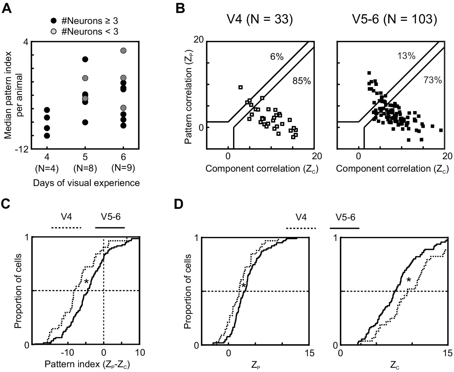
Longer visual experience results in a higher degree of PSS motion integration.

(A) Median PSS pattern index for each animal aged P37–40, plotted as a function of visual experience. Gray dots represent animals that yielded 1–2 neurons, and black dots represent animals with data for at least three neurons. (B) Pattern versus component correlations at P37–40 split according to visual experience (same plot format as Figure 2C). (Left) Animals with 4 days of visual experience. (Right) Animals with 5–6 days of visual experience. (C) Cumulative distributions of pattern indices for PSS cells in kits with 4 days (V4, dashed line) or 5–6 days (V5-6, solid line) of visual experience. *p<0.05. (D) Cumulative distributions for component correlation (left) and pattern correlation (right) for the two groups. *p<0.05.

Figure 3—source data 1 Neuron-by-neuron metrics for Figure 3.: https://cdn.elifesciences.org/articles/59798/elife-59798-fig3-data1-v2.xlsx
Download elife-59798-fig3-data1-v2.xlsx

The above analysis relies entirely on natural variation in eye opening across animals. While this offers the advantage of studying the impact of visual experience outside of artificial manipulations, it limits the available data set. For example, certain combinations of gestational age and visual experience duration did not occur in our data set. In addition, some correlation between eye opening and gestational date is unavoidable and resulted in the fact that animals in the V4 group were slightly younger (mean age 37.6 days, range 37–40) than animals in the V5–6 group (mean age 38.6, range 37–40). We therefore tested whether visual experience indeed had an effect in addition to age by performing a two-way ANOVA on the pattern index data from all PSS cells with factors visual experience (V4–V6) and age (P37–40). Main effects for both factors were significant (main effect age: p=0.02; main effect visual experience: p=04), demonstrating that both contributed significantly to the observed variance in pattern index across cells. Due to the sampling limitations imposed by natural variability, additional experiments will be needed to fully disentangle the impacts of age and experience. Yet, our results suggest that visual experience impacts the development of PSS motion integration, in addition to the contribution of age.

Developmental changes in PSS plaid response strength

Our stimulus set allowed us to probe PSS plaid responses not just as a function of plaid direction, but also as a function of dOri, the intersection angle between the two component gratings. Possible reasons for a response modulation with dOri include differences in the spatial frequency of these plaids, as well as differences in their speed (Zaharia et al., 2019; Priebe et al., 2003). Additionally, the motion integration mechanisms acting in PSS will likely have an impact on plaid response strength by determining how strongly different component signals interact, an assumption that is supported by the observation that the strength of plaid responses is positively correlated with pattern index in both primate MT and adult ferret PSS (Lempel and Nielsen, 2019; Wang and Movshon, 2016).

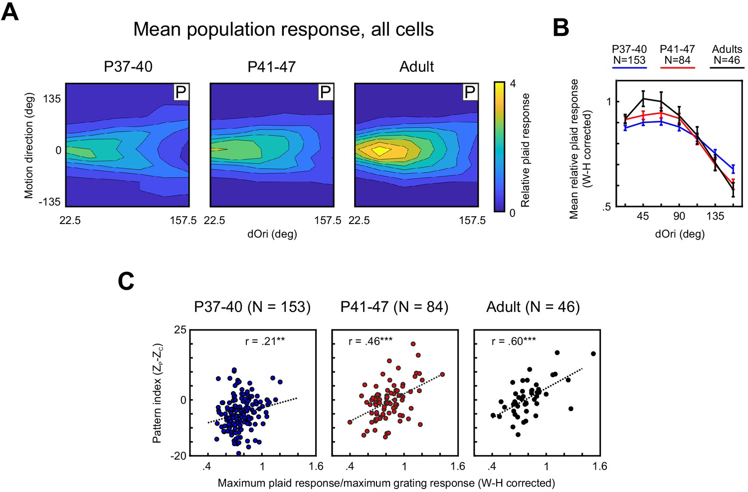
Here, we found that the dependency of response strength on dOri underwent a series of developmental changes. Figure 4A captures these changes by plotting the population tuning profile as a function of dOri and plaid direction for the different age groups, with the plaid responses of every neuron normalized by the response to gratings. We also quantified changes in relative plaid responses by averaging across all plaid directions (Figure 4B). Note that when analyzed separately for each dOri, the relative plaid response followed a χ² distribution (Figure 4—figure supplement 1). We therefore used a Wilson–Hilferty transformation (Wilson and Hilferty, 1931) to transform relative plaid responses to a normal distribution before any of the subsequent analyses. Figure 4B shows the transformed data; the raw data and effects of transformation are presented for reference in Figure 4—figure supplement 1.

Figure 4 with 1 supplement see all

Download asset Open asset

Responses of PSS neurons to plaid stimuli become increasingly modulated by dOri with development, especially in pattern cells.

(A) Average 2D profile of PSS responses to plaids at different ages (plotted in same format as Figure 1D–E). Average response profiles were computed by normalizing the data for each neuron by its mean grating response, shifting responses in direction space to center the preferred direction at 0 deg, and averaging across all neurons in each age group. (B) Average relative plaid response as a function of dOri. The average relative plaid response shown here was computed by averaging the relative plaid responses shown in (A) across all directions at each dOri. All data were transformed using a Wilson–Hilferty transformation to achieve a normal distribution at each dOri value. Error bars: ± SEM. For statistical comparisons of data across age groups, see Table 1. (C) Ratio between the maximum response to plaids of dOri = 90 deg and the maximum response to gratings versus the pattern index for all PSS neurons at different ages. Dashed lines indicate linear fits, r the correlation coefficient. Data are shown after a Wilson–Hilferty transformation. **p<0.01. ***p<0.001.

Figure 4—source data 1 Neuron-by-neuron metrics for Figure 4 and Figure 5—figure supplement 1.: https://cdn.elifesciences.org/articles/59798/elife-59798-fig4-data1-v2.xlsx
Download elife-59798-fig4-data1-v2.xlsx

Comparing the average relative plaid responses across age groups revealed that their dOri dependency systematically changed, especially between the youngest age group and both older groups. Most notably, in the youngest animals, changes in dOri caused less changes in plaid responses than in older animals. This was reflected in significant interactions between dOri and age when comparing the youngest animals against either of the other two groups using a two-way ANOVA (P37–40 vs P41–47, p=0.006; P37–40 vs Adult, p=0.004). As a post hoc test, we compared relative plaid responses between age groups at the dOri values evoking maximal and minimal responses in adults (dOri = 45 and 157 deg, respectively). At dOri = 45 deg, we observed significantly lower plaid responses in the youngest animals than in adults (p=0.005). Responses were not different from the P41–47 group for this dOri value. In contrast, responses at dOri = 157 deg were significantly higher in the youngest group than either of the other groups (P37–40 vs P41–47, p=0.02; P37–40 vs Adult, p=0.01). Thus, the post hoc tests confirm that the youngest animals showed less modulation of plaid response strength with dOri than older animals. It should be pointed out that the reduction in responses to plaids with large dOri values between P37–40 and P41–47 correlated with a large reduction in component responses (Figure 4A). In the youngest age group, the impact of the stronger component responses is visible in the clear ‘V’-shape of the population tuning profile. As could be expected, component responses were less affected by dOri, which resulted in a higher response to plaids with large dOri in the youngest age group when averaging across all plaid directions (as done for Figure 4B).

As mentioned above, the maximum relative plaid response is positively correlated with the pattern index in ferret PSS and primate MT in adult animals (Lempel and Nielsen, 2019; Wang and Movshon, 2016). This relationship also emerged with development (Figure 4C; note that these data also were transformed using the Wilson-Hilferty transformation): While the correlation coefficient between pattern index and maximum relative plaid response was significant even for the P37–40 group, Figure 4C shows the dependency between the two variables was quite weak at this age. The correlation coefficient in the older age groups was significantly higher (P37–40 vs P41–47, p=0.02; P37–40 vs Adult, p=0.003), with a more obvious relationship between the two variables apparent in adults (Figure 4C). In summary, not only did the prevalence of pattern responses to plaids increase between P37–40 and P41–47, the dependency of this response on plaid configuration and pattern index developed as well, showing more comprehensive changes in how the visual system handles stimuli consisting of multiple interacting components.

Developmental changes in V1 plaid responses

Processing of stimuli in V1 is likely an important precursor to PSS functions. V1 does not just compute the local direction signals for the plaid components, the response to these components is modulated by interactions between the plaids through mechanisms like cross-orientation inhibition and motion opponency. These V1 mechanisms could further drive modulations in plaid response strength, in addition to the PSS mechanisms discussed above. We therefore sought to identify developmental changes in V1 plaid processing to gain a more complete picture of the development of the motion pathway as a whole. Accordingly, we recorded V1 responses to plaids at different ages. We selected two age groups for these experiments. The first covered the same age range as the youngest PSS animals, P37–40. The second group covered P44–47, chosen to coincide with the end of the age range of the second PSS group so as to maximize our ability to detect age-dependent differences.

Recording V1 responses to plaids revealed a series of developmental changes. First, we observed changes in the strength of plaid-evoked responses (Figure 5A,B). Between the two younger age groups, responses to plaids generally increased independent of dOri (two-way ANOVA, contribution of age p=0.001), before decreasing strongly in adults. With the decrease in adults also came some changes in the dOri-driven response modulation, as evidenced by significant interactions between dOri and age when comparing the P44–47 age group with the adults using a two-way ANOVA (contribution of age, p<0.001. interaction, p=0.03). The overall decrease in V1 plaid responses was very pronounced in our data set. Note, however, that a previous study (Popović et al., 2018) investigating the development of V1 cross-orientation inhibition in ferrets (i.e., looking at responses to plaids with dOri = 90 deg) did not observe changes in plaid responses between P40 and adulthood, something that will need to be resolved with further experiments (see also Discussion).

Figure 5 with 1 supplement see all

Download asset Open asset

V1 responses to plaids change during PSS motion integration development.

(A) Average 2D profile of responses to plaids in V1 at different ages (computed and plotted as in Figure 4A). (B) Average relative plaid response in V1 as a function of dOri (data shown after Wilson–Hilferty transformation; same format as Figure 4B). Error bars: ± SEM. (C) Pattern versus component correlations for V1 neurons in different age groups (same format as Figure 2C). (D) Cumulative distribution plots for V1 pattern indices at different ages. Same N and color scheme as (C).

Figure 5—source data 1 Neuron-by-neuron metrics for Figure 5 and Figure 5—figure supplement 1.: https://cdn.elifesciences.org/articles/59798/elife-59798-fig5-data1-v2.xlsx
Download elife-59798-fig5-data1-v2.xlsx

Second, we made an unexpected discovery in our V1 data set: In adult animals, V1 was strongly dominated by component responses (see Figure 5E,F and Lempel and Nielsen, 2019). The same held true for the youngest age group: Across the P37–40 animals, we observed a similar number of pattern and component cells as in adults (pattern: 4% versus 3%, component: 87% versus 95%; Figure 5E), and the pattern index distributions for both groups closely aligned (Figure 5F). However, the middle age group deviated from this pattern. Across animals aged P44–47, we observed a larger number of pattern cells (15%), and the pattern index distribution was significantly shifted toward stronger integration (p<0.001). It should be noted that even with this shift V1 pattern indices remained significantly lower on average than PSS pattern indices (Figure 5—figure supplement 1, p<0.001). The same was true also for the two other age groups (p<0.001 for both groups). Taken together, our data suggest a temporary change in V1 plaid responses, characterized by stronger integration of the two component directions and weaker inhibition caused by the simultaneous presence of two gratings. The combination of these two changes had an interesting consequence: V1 responses were enhanced for plaid conditions in which the pattern motion was in the preferred direction, but were left largely unchanged for conditions in which the components moved in the preferred direction (Figure 5A). Thus, increases in response strength were largely reserved for pattern responses.

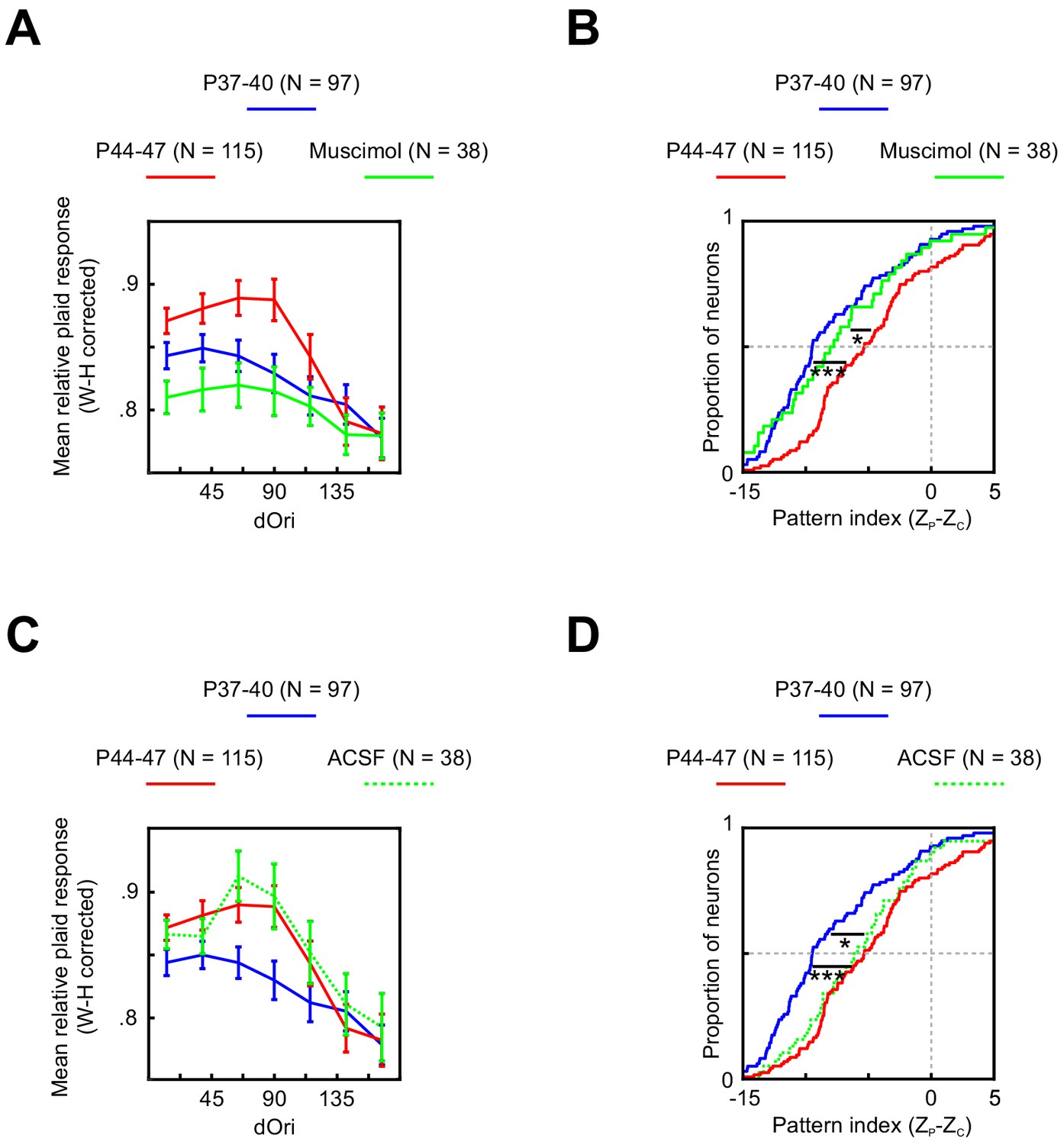
In an effort to identify possible sources for these changes, we next recorded V1 plaid responses at P44–47 while inactivating PSS with the GABA_A agonist muscimol. Inactivating PSS reversed both temporary changes in V1 plaid responses (Figure 6A,B). The relative plaid response strength was significantly reduced relative to control data (ANOVA normal versus muscimol p<0.001), reaching the same levels seen normally at P37–41. Similarly, PSS inactivation resulted in a significant shift of the pattern index to lower values (p=0.01) that matched both younger and older animals (see Table 1 for statistics). A sham PSS injection without muscimol (Figure 6C,D) did not impact V1 relative plaid responses or pattern indices (see Table 1 for statistics), confirming that PSS inactivation, rather than side effects of the injection, caused the observed V1 effects. Thus, both changes in V1 plaid responses are at least partially dependent on feedback from PSS.

Figure 6

Download asset Open asset

Changes in V1 responses at P44–47 depend on feedback from PSS.

(A) Average relative plaid response in V1 at P37–40 (same data as Figure 5B), P44–47 (same data as Figure 5B), and P44–47 with muscimol inactivation of PSS. Error bars indicate ± SEM. Data are shown after a Wilson–Hilferty transformation. For statistical analysis of data across age groups, see Table 1. (B) Cumulative distribution of V1 pattern indices at P37–40 (same data as Figure 5D), P44–47 (same data as Figure 5D), and P44–47 with muscimol inactivation of PSS. For statistical analysis of data across age groups, see Table 1. *p<0.05. ***p<0.001. (**C, D**) Same plots as (A, B) but after a control injection of ACSF into PSS. Note that the ACSF group included one animal aged P48, making the age range for this group P44–48.

Figure 6—source data 1 Neuron-by-neuron metrics for Figure 6.: https://cdn.elifesciences.org/articles/59798/elife-59798-fig6-data1-v2.xlsx
Download elife-59798-fig6-data1-v2.xlsx

Modeling the relative impact of developmental changes in V1 versus PSS on motion integration

As described in the previous section, we observed temporary changes in V1 plaid responses between P44 and P47. The results of the inactivation experiments indicate that these changes depend on feedback from PSS. At the same time, changes in V1 presumably propagate to PSS (and more generally areas downstream from V1), potentially initiating changes in plaid processing throughout the motion pathway. What consequences could the V1 changes have on motion integration computations in PSS, in particular relative to developmental processes occurring within PSS? Obviously, this question will need to be answered experimentally, but as a first step toward providing some answers we made use of a computational model for the motion pathway.

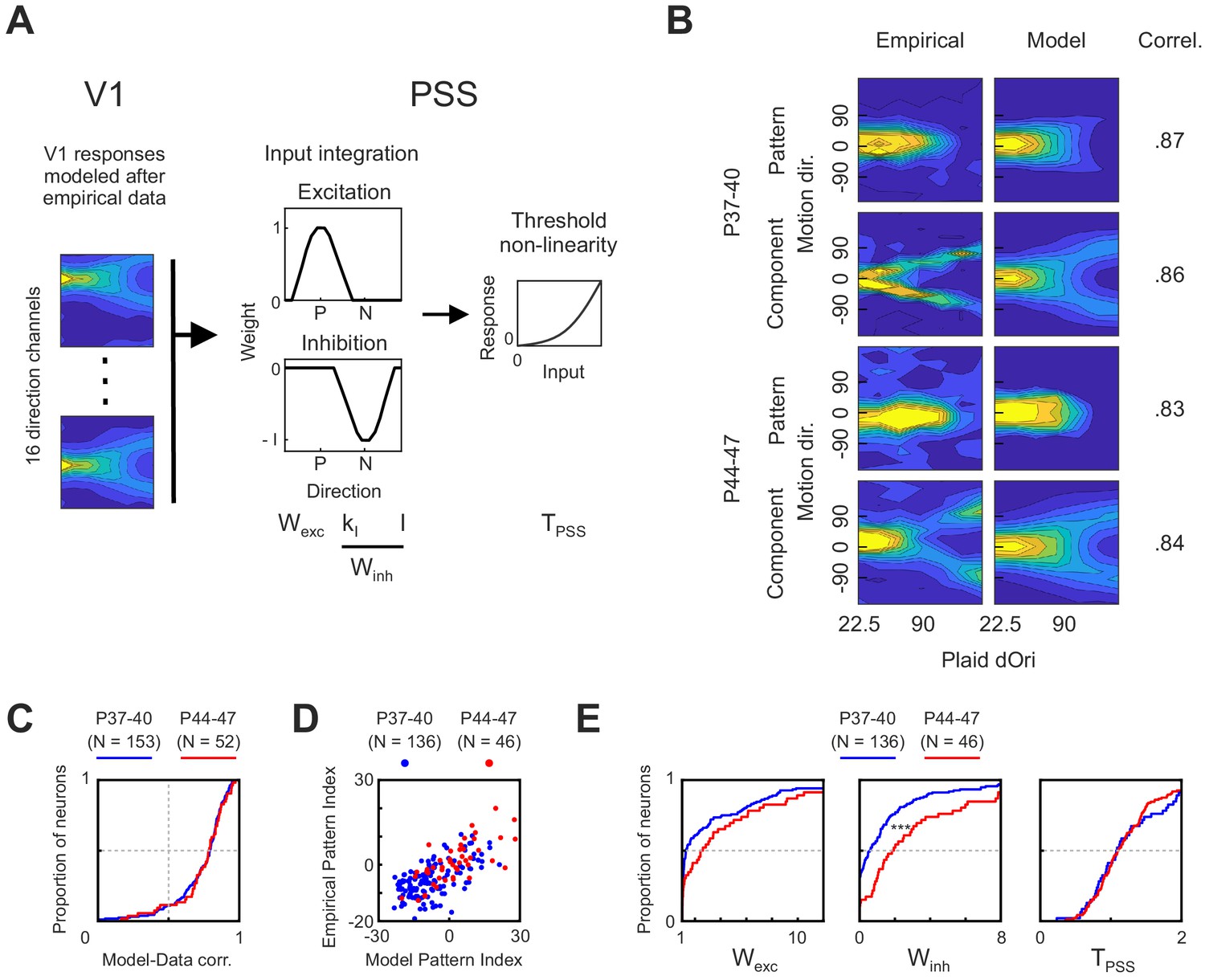
We have previously shown that a two-stage model consisting of V1-like local direction filters followed by a PSS-like integration stage could fit well to neural responses in PSS (Lempel and Nielsen, 2019). Here, we used a modified version of this model to investigate development. Since the goal was to identify the contribution of particular V1 and PSS changes, we replaced the front end of the model. Rather than adjusting the parameters of the V1 stage as needed for the best fit to a given PSS neuron, we fixed it to match the experimentally observed data. More precisely, in the model implemented here (see Figure 7A), the first stage was set to be a bank of 16 direction filters that when exposed to plaids would reproduce our measured average V1 responses as closely as possible, including their dOri dependence. Two modifications were made to the empirical V1 response profile in building the model V1 filters: First, we made responses symmetric around the preferred direction. Second, motion pathway models usually assume perfect direction tuning in the V1 stage (i.e., no responses to stimuli moving in the null direction). We similarly modified the V1 response profile to achieve maximal direction tuning (see Materials and methods for details).

Figure 7

Download asset Open asset

A computational model of the ferret motion pathway for testing mechanisms behind motion integration development.

(A) Diagram of the model used to explain PSS plaid responses across development. The first stage was composed of 16 V1 direction selective cells whose responses were modeled after empirical V1 data from different age groups. Responses from the V1 stage were then integrated in PSS using a combination of an excitatory and an inhibitory weight function (P, preferred direction; N, null direction). Finally, an exponential non-linearity was applied to the PSS responses. The model had four variables, which are listed below the stage to which they belong. For analysis of model results the two variables controlling inhibition (K_I and I) where combined into a single metric (W_inh, see Materials and methods). (B) Examples of empirical PSS responses to plaids (left column) and corresponding model PSS responses (right column) after optimizing model parameters to maximize the likelihood of the empirical data for each neuron. Examples show one pattern and one component cell from animals before (P37–40) and after (P44–47) development of motion integration in PSS. Numbers to the right of response profiles indicate correlation between model and empirical responses. (C) Distribution of correlation coefficients between model and empirical responses for each PSS neuron in the two age groups. Results from neurons with model-data correlation below 0.5i were excluded from further analyses. (D) PSS pattern index for every neuron, computed using empirical data or model data for the neuron, for both age groups. (E) Cumulative distribution of all model variables after fitting the model to data from kits before (P37–40) and after (P44–47) the development of motion integration. ***p<0.001.

Figure 7—source data 1 Neuron-by-neuron metrics for Figure 7.: https://cdn.elifesciences.org/articles/59798/elife-59798-fig7-data1-v2.xlsx
Download elife-59798-fig7-data1-v2.xlsx

The PSS integration stage of the model remained identical to our previous study. In this stage, the responses of the 16 V1 direction channels were integrated using a weight function with an excitatory component centered at the preferred direction and an inhibitory component centered at the null direction. Both components were modeled as von Mises functions. The width of the excitatory component, as well as the width and amplitude of the inhibitory component were free model parameters. Below, they are summarized as W_exc and W_inh, which refer to the area under the excitatory and inhibitory component, respectively. The integration stage finally was followed by an exponential non-linearity determined by the free parameter T_PSS. Note that one major purpose of the model was to test whether the observed V1 changes could propagate to PSS (and how they would affect PSS responses). For this reason, the model remained strictly feedforward, despite the above observations that V1 changes depended on feedback from PSS. Future models will need to expand to more complicated models including both feedforward and feedback links to fully explore the dependencies between areas.

As a first modeling exercise, we attempted to identify which PSS-internal mechanisms might explain the developmental changes occurring after P40. To this end, we set the V1 stage to the data measured between either P37–40 or P44–47 and then used a maximum likelihood approach to fit the model to PSS responses measured in the same age range (see Materials and methods). Note that because the V1 data only covered P44–47, we restricted the PSS data set to the same range for the modeling analysis. As illustrated by the example pattern and component cells shown in Figure 7B, the model was well able to fit PSS neurons of different types at both ages. This was further confirmed by a generally high correlation between modeled and measured data for both groups, with little differences between the groups (Figure 7C). In all subsequent analyses, we excluded cells with correlation coefficients below 0.5. For both age groups predicted and measured pattern indices generally matched well (Figure 7D). While the model generally overestimated the absolute value of a neuron’s pattern index, likely because of lower noise levels in the modeled responses, pattern cells remained classified as pattern cells based on the model fits, and component cells remained classified as component cells.

The good model fit for both age groups allowed us to compare model parameters across ages. Cumulative distributions for W_exc, W_inh and T_PSS are plotted for both age groups in Figure 7E. These plots show a trend toward increasing W_exc with age, but the difference between age groups did not reach significance (p=0.06). At the same time, W_inh significantly increased between the two groups (p<0.001). T_PSS, finally, remained unchanged. Thus, the model results suggest that changes in PSS null direction inhibition are a major component of motion integration development.

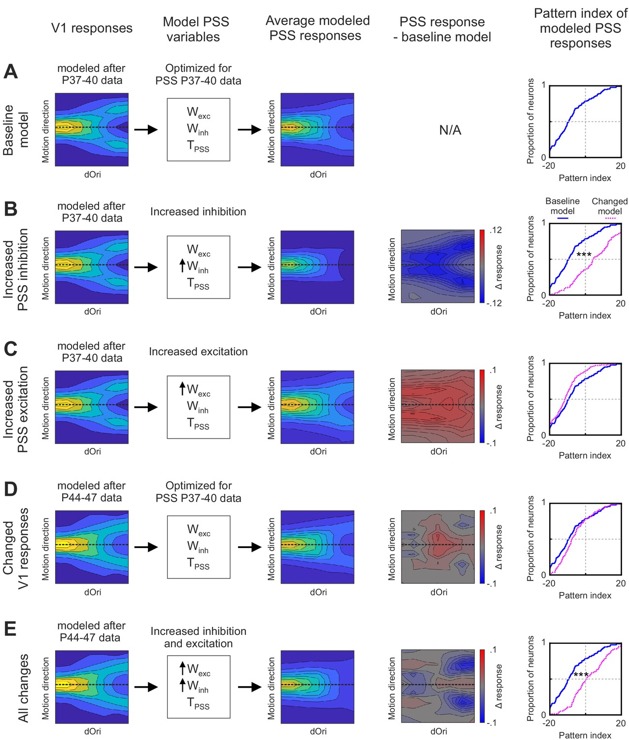
Having identified the major changes internal to PSS that could be driving motion integration development, we next sought to determine how the temporary V1 changes complemented them. To this end, we used the following stepwise procedure: We first initiated the model with its state at P37–40. In this baseline model, the V1 stage was set to match the empirical data for P37–40, as shown in the first column of Figure 8A. We also set the parameters for the PSS stage to those determined by fitting the model to PSS data from the same age group. One set of parameters was computed for each neuron in the data set (N = 136), allowing us to construct a population of model PSS neurons. The resulting model PSS responses are summarized in Figure 8A by plotting the average plaid response profile for all PSS model neurons (third column), as well as the resulting pattern index distribution (fifth column).

Figure 8 with 1 supplement see all

Download asset Open asset

Effects of changes in V1 and PSS mechanisms on PSS plaid responses.

Summary of different instantiations of the motion pathway model. (A) Baseline model. (B) Model with increased PSS inhibition. (C) Model with increased PSS excitation . (D) Model with V1 responses set to reflect those measured at P44–47. (E) Model combining all changes described for (B), (C), and (D). For each model instantiation, the columns (from left to right) contain the following information: Colum 1: V1 plaid responses used for the model’s first stage. Dashed line indicates the preferred motion direction. Column 2: State of PSS parameters for motion integration (W_exc), inhibition (W_inh), and threshold non-linearity (T_PSS) relative to the baseline model (determined by fitting the model to data from P37–40). No arrow indicates values were unchanged relative to the baseline model, upwards arrow indicate an increase in the parameter. Column 3: Average plaid responses of model PSS neurons. Dashed line indicates the preferred motion direction. Column 4: Difference between average plaid responses of model PSS neurons in a model instantiation and the average response in the baseline model. Column 5: Cumulative distribution of pattern indices of model PSS neurons for the new model instantiation (dashed pink line) and baseline model (solid blue line). ***p<0.001.

Figure 8—source data 1 Neuron-by-neuron metrics for Figure 8 and Figure 8—figure supplement 1.: https://cdn.elifesciences.org/articles/59798/elife-59798-fig8-data1-v2.xlsx
Download elife-59798-fig8-data1-v2.xlsx

We then used modifications of the baseline model to assess the impact of different developmental changes. First, we asked what contributions the increase in PSS null direction inhibition made to pattern responses. In this model iteration, we kept the V1 stage unchanged relative to the baseline model, that is, it remained set to mimic responses at P37–40. At the same time, we adjusted W_inh of the PSS stage to match the levels seen at P40–44. To achieve this, we increased the value of the model parameter I, which controls the strength of inhibition (see Materials and methods), so that the new mean W_inh value equaled that determined when fitting the model to data for P40–44 (Figure 8—figure supplement 1; note that we did not adjust K_I since it showed little differences between ages in the original fit). Figure 8B shows the resulting average PSS plaid response profile (third column) and pattern index distribution relative to that of the baseline model (fifth column). It also shows the response difference between the new model iteration and the baseline version as a function of plaid direction and dOri (fourth column). These figures demonstrate that while increasing PSS inhibition resulted in a large overall increase in pattern indices, it came with reduced plaid responses. On the one hand, responses were weakened for plaids in which one of the conditions (but not the integrated plaid) moved in the preferred direction (these make up the arms of the ‘V’-shaped response profile). Changes to these conditions will increase pattern responses by decreasing component responses and are the key mechanism by which inhibition can shape pattern responses. On the other hand, the increased inhibition extended to conditions in which the pattern movement was in the preferred direction, in particular for intermediate dOri values (likely because for these conditions the components were far enough from the preferred direction to experience some of the increased null direction inhibition). Thus, the improvement in pattern index by increased inhibition came at a cost.

In the second model iteration, we assessed the impact of increasing the excitatory integration of component signals in PSS. While the changes in W_exc between P37–40 and P44–47 failed to reach significance, excitation levels nonetheless showed a moderate increase between these two groups. Here, we kept all model parameters with the exception of K_E, the only parameter controlling excitation, fixed in their baseline state. K_E was decreased (which has the effect of broadening the excitatory part of the integration function, thereby increasing W_exc) until the mean of the model W_exc distribution matched that determined previously in the P44–47 model fit (Figure 8—figure supplement 1). Figure 8C again plots the resulting model PSS response to plaids, the difference to the baseline model, and the new pattern index distribution. Increasing excitation actually decreased the pattern index by diminishing differences between pattern and component responses, but as expected, the strength of pattern responses was increased across all dOri values.

In the third model iteration, we then asked what contribution the observed temporary changes in V1 would make to PSS pattern responses. In this iteration, we changed the V1 stage to match the data measured in P44–47 animals, while fixing the PSS model parameters to the values determined for P37–40. The new V1 response profile is plotted in Figure 8D, as is the resulting average PSS response profile, its difference relative to the baseline model, and the resulting pattern index distribution. We found that changing the V1 stage on its own had little consequences on PSS pattern indices, which remained largely unchanged from the P37–40 baseline model. However, there were changes in the PSS response to plaids. The selective increases in V1 pattern responses indeed propagated to PSS and resulted in increased responses for pattern motion for plaids with intermediate dOri values.

Finally, we combined V1 and PSS changes in the fourth model iteration to determine their combined effect (Figure 8E). The major difference between this model iteration, and a full fit of the pathway model to data from P44 to P47 as performed in Figure 7, was the state of the PSS stage. Rather than optimizing these parameters through fitting the model, we only shifted the mean inhibition and excitation levels of the baseline model as described above. In this last model iteration, the increases in inhibition again served to decrease component responses and increase the pattern index. At the same time, increases in PSS excitation, combined with the changes in V1 plaid responses, mitigated the side effects of the increased suppression levels by limiting them to the component responses only.

Discussion

A hallmark of cortical organization is the existence of specialized pathways dedicated to certain kinds of information processing. Here, we use motion integration – in the form of local and global motion signals to coherent plaids – to characterize the development of the visual motion pathway. On a basic level, our data reveal that motion tuning functions develop according to their complexity: Direction selectivity in V1 and PSS matured before motion integration. This matches findings in the primate, in which MT pattern cells also develop slowly, over the course of months, after direction selectivity develops (Chino et al., 1997; Kiorpes and Movshon, 2014).

Intriguingly, our data suggest that visual experience has an impact on the development of PSS motion integration. These findings add to an existing body of work on the role of visual experience in the development of the carnivore motion pathway. In both ferrets and cats, visual experience is required for normal development of direction selectivity in V1 (Li et al., 2008; Blakemore and Van Sluyters, 1975; Cynader et al., 1976). At least the basic functions in higher areas are also susceptible to a lack of normal visual experience: Rearing cats in a stroboscopic environment, in which normal motion cues are removed, results in the loss of direction selectivity in higher area PMLS (Spear et al., 1985). Our data point to a role of visual experience in the development of the more complex functions of these higher areas as well. Since the animals here were raised under normal conditions, the current data can only show that visual experience can accelerate the development of these functions. Additional experiments are needed to test whether it is actually necessary. However, our findings are consistent with the observation that dark reared cats have marked deficits in a behavioral motion integration task (Mitchell et al., 2009). The impact of visual experience on the development of motion integration has also been investigated in the primate. At this time, evidence for a role of visual experience on these functions is mixed: Neurons in MT of amblyopic monkeys show no changes in pattern responses for plaids, but changes in global motion processing were observed when using random dot kinematograms (RDK) (El-Shamayleh et al., 2010). It remains to be determined whether a more severe loss of visual experience, as in the carnivore studies, would result in larger deficits in MT functions. Indeed, bilateral congenital cataracts cause large deficits in motion integration performance for RDK in humans, but deficits after monocular cataracts are much smaller (Ellemberg et al., 2002).

With the development of motion integration came a change in how the plaid configuration modulated PSS responses. In part, these changes might reflect the development of spatial and temporal tuning functions in PSS, which remain to be studied longitudinally. More generally, it is currently unknown whether PSS neurons are tuned for temporal frequency or speed and how these tuning properties interact with the pattern index, as has been investigated for MT (Zaharia et al., 2019; Priebe et al., 2003). However, the developmental change in dOri dependency of PSS responses likely reflects at least in part the maturation of motion integration mechanisms. An increase in response to plaids with smaller to intermediate dOri values, for example, is consistent with increasingly stronger interactions between different motion signals that are pooled together to compute pattern motion. This conclusion is further supported by the observation that plaid responses became stronger especially in pattern cells throughout development.

While motion integration mechanisms in PSS are obviously crucial to shaping plaid responses, PSS does not exist in isolation, but receives input from other areas. Our V1 data highlight that processing even in supposedly earlier areas of a pathway should not be treated as mature or static when studying development of a higher area. Here, we found temporary changes in the degree of V1 motion integration around P44–47 and more continuous changes in plaid response strength throughout development. Our model (see also below) shows that these changes might serve an important role in conjunction with developmental changes in PSS. At the minimum, characterizing V1 responses provides a benchmark against which to assess PSS development. Note that our data show a large decrease in V1 plaid responses – that is a large increase in cross-orientation inhibition – between P44–47 and adults. Cross-orientation inhibition has previously been studied for 90 deg plaids in ferret V1, both at P40 and in adult animals (Popović et al., 2018). In this previous study, relative plaid responses were reported as the ratio between the preferred plaid and the sum of responses to the components. Using the same metric, we observe similar levels of cross-orientation inhibition around P40 (in the new metric, our data has a mean of 0.21 for plaids with dOri = 90 deg). However, the two data sets diverge strongly for adult animals. While our data show a strong increase, Popovic et al. report a small but significant decrease in cross-orientation inhibition. This discrepancy may be due to differences in the sampled neuronal population (in terms of laminar location or location within V1), but it is more likely caused by differences in the stimulus presentation protocol (slower presentation of individual stimuli versus fast presentation embedded in a train of stimuli). Resolving these differences will require additional experiments in adult animals, which will also need to address why these differences only occur for adults.

Our model suggests a possible role for the temporary V1 changes we observed. More precisely, the model results show that the changes in V1 responses can complement changes in PSS-internal motion integration mechanisms in a meaningful manner. We modeled PSS motion integration by using a weight function with an excitatory component centered at the preferred direction, and an inhibitory component centered at the null direction. This was motivated by the importance of null direction inhibition in motion computations in ferret V1 (Wilson et al., 2018), but it also matches the shape of MT motion integration functions as estimated by fitting a primate motion pathway model to plaid responses (Rust et al., 2006). Inhibition proved to be the strongest contributor to improving motion integration. Increasing inhibitory levels from those at P37–40 to the levels at P44–47 strongly increased the pattern index across the entire model neuron population. Our model therefore makes the testable prediction that inhibitory circuits in PSS should mature relatively slowly, not before P40. No data exist for inhibitory circuit development in PSS, but inhibitory circuits in ferret V1 have been found to develop up to P60 both in terms of the relative proportion of different types of inhibitory neurons, as well as their laminar distribution (Chen et al., 2005; Dalva, 2010; Gao et al., 1999; Gao et al., 2000). A similarly slow development of inhibitory circuity in PSS does therefore appear possible.

The change in pattern index due to increased inhibition was largely driven by a reduction of component responses. However, the increased inhibitory levels necessarily came at a cost, causing reduction in pattern responses as well. It could be expected that increasing the excitatory integration component in PSS could mitigate these effects. However, there is a limit to how much this component can be changed: The unwanted suppression of pattern responses occurs in particular for plaids with intermediate dOri values. To increase the responses to these plaids, the excitatory component would need to increase in width – but the broader this part of the weight function, the broader the resulting direction tuning function even for simple stimuli like gratings. By dividing the ‘workload’ of increasing pattern responses between V1 and PSS, the increases in the excitatory weight function in PSS can be kept to a reasonable level. In this context, it is worth reiterating an observation regarding the V1 changes: Because V1 responses became more biased toward pattern responses as they became stronger at P44–47, they boosted pattern responses to the preferred direction only, rather than affecting all conditions. Thus, independent of the exact implementation of the motion pathway model, V1 selectively contributes to strengthening responses to the plaid conditions most important for pattern motion computations.

Additional experiments are required to investigate whether V1 changes are necessary for normal PSS development, how they interact with visual experience, and how other areas beyond V1 and PSS contribute to motion pathway development. The temporary nature of the V1 changes (at least in our data set) also poses interesting questions. If V1 changes are indeed temporary, it would suggest that other mechanisms – originating either in PSS or elsewhere – eventually replace the V1 contribution. Alternatively, V1 changes may actually be permanent, but become limited to the subgroup of neurons that project from V1 to PSS, similar to the other specializations that have been reported for the V1 neurons participating in the motion pathway (Jarosiewicz et al., 2012; Movshon and Newsome, 1996).

Finally, and most importantly, we have discussed the impact of V1 changes in a purely feedforward context so far. Yet, our inactivation experiments demonstrated that these changes depended on feedback from PSS. Independent of their potential consequences on PSS processing, these findings raise two interesting possibilities (which are not mutually exclusive): In one scenario, PSS actively adjusts V1 signals to (temporarily) aid its own development. In the other, V1 changes are a (more passive) consequence of the change in PSS feedback signals that arises from the newly developed PSS functions. Either scenarios link development across multiple network nodes of the motion pathway, and are important concepts for studying the development of a cortical pathway.

Materials and methods

Animal preparation and surgery

Request a detailed protocol

All procedures adhered to the guidelines of the National Institute of Health and were approved by the Animal Care and Use Committee at Johns Hopkins University. Experiments were performed in both male and female sable ferrets (Mustela putoris furo) aged 37–448 days. Experiments were conducted in anesthetized ferrets, using the same procedures as described in our previous work (Lempel and Nielsen, 2019). Briefly, animals were anesthetized during the experiments using isoflurane (during surgery: 1.5–3%, during recording: 0.5–2%) and paralyzed using pancuronium bromide (0.15 mg/kg/hr). A number of vital parameters (heart rate, SpO2, EKG, EtCO2, and the EEG) were monitored continuously to ensure adequate anesthetic depth during the experiments. Neosynephrine and atropine were applied to the eyes to retract the nictitating membrane and dilate the pupil, and animals were fitted with contact lenses. Before recordings, craniotomies were made above either V1 or the posterior bank of the suprasylvian sulcus to reach PSS. We targeted central visual field regions in V1, and central and more peripheral visual field regions in PSS.

Electrophysiology

Request a detailed protocol

Neural signals were recorded using either custom-made tetrodes (12 µm nichrome wire, gold-plated to reach final impedances of 150–500 kΩ) or 64-channel silicon microprobes obtained from the Masmanides lab at UCLA (Du et al., 2011). Probes were gold-plated to reach final impedances of 150–300 kΩ. Signals were amplified and recorded using a CerePlex Direct amplifier (Blackrock Microsystems) or a RHD2000 amplifier (Intan Technologies). Raw data were acquired at either 30 or 20 kHz and filtered between 250 Hz and 5 kHz. Spike detection threshold was set manually for each recording based on noise levels. Single-unit isolation was performed off-line using MATLAB (MathWorks). Isolation was based on multiple waveform characteristics (e.g., spike amplitude peak, area under the waveform, repolarization phase slope) recorded on the four tetrode channels or on neighboring channels of the silicon probe. Quality of isolation was confirmed by inter-spike interval (ISI) analysis. Units that displayed ISIs below 1.2 ms were not included in further analyses.

Muscimol injections

Request a detailed protocol

PSS was inactivated by injecting muscimol (2.5 mg/ml in ACSF; Sigma) in multiple sites spanning the posterior bank of the suprasylvian sulcus. For control experiments, ACSF without muscimol was injected instead. To aid the visualization of injection location and spread, 0.05% Fast Green FCF (Fisher Scientific) was added to both the muscimol and control solution. To inject the solution, we used glass pipettes pulled using a micropipette puller (Sutter instrument, model P-1000) and 5 µl calibrated glass capillary tubes (VWR). Infusion was performed at a rate of 0.1–0.5 µl/min. For each animal, injections were performed at four different locations along the posterior bank of the suprasylvian sulcus. At each location, 0.2–0.4 µl of either muscimol or ACSF solution were infused at 4 depths spaced 200–300 µm apart. In total, 4–5 µl of either muscimol of ACSF solution were injected per animal. Recordings were made in V1 1–5 hr after injection. For muscimol experiments, lack of PSS responsiveness was confirmed by extracellular recordings either during or right after the last V1 recording.

Visual stimuli and experiment design

Visual stimuli were generated using the Psychophysics Toolbox extensions for MATLAB (Brainard, 1997; Pelli, 1997) and displayed on a 24-inch LCD monitor with a refresh rate of 120 Hz, placed 25–35 cm in front of the ferret. For a subset of experiments, a 43-inch LCD monitor with a refresh rate of 60 Hz was used instead. Monitors were gamma corrected using a SpectraScan 655 (PhotoResearch).

Measurements of direction selectivity

Request a detailed protocol

The direction selectivity data shown in Figure 1—figure supplement 1 was collected in a set of separate experiments. These experiments consisted of gratings moving in different directions as well as a blank condition. Each condition was repeated five times, with conditions presented in a pseudo-random sequence. Measurements of direction selectivity at P37 used square-wave gratings. In adults, either square-wave or sine-wave gratings were used to measure direction selectivity. Square-wave gratings were only used for the direction selectivity measurements shown in Figure 1—figure supplement 1, and not for any of the subsequent plaid experiments. Grating spatial frequency was set to maximize responses at the recording location (range 0.05–0.1 cycles/deg), as was temporal frequency (range 2–6 Hz). Gratings were shown at 100% contrast and moved in 12 or 16 different directions. Stimuli were presented interspersed with presentation of a gray screen of equal mean luminance. Stimuli were presented for 1 s with inter-stimulus intervals of 2–10 s and at a size of 65 × 50 deg.

Plaids, classic stimulus presentation

Request a detailed protocol

These experiments consisted of plaids and gratings. Gratings in these experiments were sine-wave gratings of optimal spatial and temporal frequency shown at 50% contrast. Plaids were generated by superimposing two 50% contrast sine-wave gratings of the same spatial and temporal frequency at an intersection angle of 135 deg. Both gratings and plaids could move in 16 different directions. Five repetitions of each stimulus condition were shown. Stimulus sizes were optimized for each neuron. For most experiments, stimuli were shown in a circular aperture with radius 8–30 deg, but in a small subset of adult plaid experiments, we used rectangular stimuli of 65 × 50 deg instead. Otherwise stimulus parameters were set as described above.

Plaids, streaming stimulus presentation

Request a detailed protocol

Each trial consisted of a 60 s long sequence of short stimulus presentations (3–4 stimuli/s). Each sequence was preceded and followed by a 2–4 s long presentation of a gray screen of equal luminance. Stimulus sequence was determined randomly by picking from all stimulus conditions with replacement. The following stimulus conditions were used: blank (uniform gray screen), 100% contrast sine-wave gratings moving in 16 directions, and plaids with seven different component intersection angles (dOri = 22.5, 45, 67.4, 90, 112.5, 135, and 157.5 deg) moving in 16 directions. In a subset of experiments, we also included 50% contrast gratings moving in 16 directions. Spatial frequency (0.05–0.15 cycles/deg), temporal frequency (3–6 Hz), and stimulus size (circular aperture of radius 10–35 deg) were optimized at each recording location. For each stimulus, the initial phase of each grating was chosen randomly from four possible values (0, 90, 180, and 270 deg). Thirty or 45 trials were run for each experiment, so that each stimulus was presented at least 10 times.

Data analysis

Direction selectivity and classic stimulus presentations for plaids

Request a detailed protocol

For direction selectivity measurements and experiments using the classic stimulus presentation mode (Figure 1—figure supplement 1 and Figure 2), neuronal responses were calculated as the firing rate during stimulus presentation minus the firing rate during the last second of the pre-stimulus period. Tuning properties were then computed based on the mean responses across stimulus repetitions for each condition.

Direction selectivity was quantified using a direction index comparing responses between preferred and null directions, which was computed as follows:

D S I = 1 - \frac{R (N)}{R (P)}

where R(P) is the response to the preferred direction and R(N) is the response to the null direction. We also computed an orientation selectivity index, which was used for cell selection in the plaid analysis (see below). This index was computed as follows:

O S I = 1 - \frac{R (O)}{R (P)}

where R(P) is the response to the preferred direction and R(O) is the mean response to the two gratings with an orientation orthogonal to the preferred. Both indices are computed based on responses to gratings only.

To quantify motion integration in the classic paradigm, we used standard methods to compute partial correlations between the measured plaids responses and pattern and component response predictions (Movshon et al., 1985). Partial correlations were then Z-transformed to achieve a normal distribution that takes into account the degrees of freedom and better allows comparisons across conditions. The Z-transform was computed as (Smith et al., 2005):

Z = \sqrt{N - 3} \frac{1}{2} ln (\frac{1 + r}{1 - r})

where r is the partial correlation (either pattern or component) and N refers to the number of points in the correlation (here, 16). Cells were classified as pattern cells if they met Z_P – Z_c >1.28 for Z_C ≥0, and Z_P >1.28 otherwise. Component cells had to meet the opposite criterion. We also computed a pattern index as Z_P–Z_C. As in the cell classification, any negative values (Z_P or Z_C) were set to 0 when computing the index.

Streaming stimulus presentation

Request a detailed protocol

Stimulus-evoked responses collected using the streaming stimulus paradigm were extracted after computing an optimal latency for every neuron, as described in our previous work (Lempel and Nielsen, 2019). After computing the response to each condition, each neuron’s pattern and component predictions were computed as described in Lempel and Nielsen, 2019. Briefly, we computed a dOri curve for every neuron as the average across all stimuli with the same dOri. We then combined the dOri curve with a direction tuning curve to generate a pattern and component prediction. For the pattern prediction, this direction tuning curve was computed by averaging responses to gratings and plaids with shared directions, using the pattern direction as the plaid’s direction. For the component prediction, the direction tuning curve was instead computed based on the component directions (again, gratings were included in this computation). Finally, we computed partial correlations of each neuron’s actual response with the two predictions and converted these values to Z-scores as before (with N set to 112 to account for the 7 dOri values and 16 directions involved in the computation).

Inclusion criteria and data set size

Direction selectivity and classic stimulus presentations for plaids

Request a detailed protocol

For direction selectivity measurements and experiments using the classic stimulus presentation mode (Figure 1—figure supplement 1 and Figure 2), we first excluded neurons that did not meet a minimal response criterion by eliminating all neurons for which the best condition had an average firing rate of less than 2 Hz. The remaining neurons were then screened for general stimulus responsiveness. For direction selectivity measurements (Figure 1—figure supplement 1), we performed this test by using a one-way ANOVA to compare responses across all stimulus conditions (including the blank). Only cells that passed p<0.01 for the ANOVA were included in further analyses. For the plaid experiments (Figure 2), two responsiveness tests were performed: one for gratings and one for plaids only. Both tests used a one-way ANOVA to compare responses across all stimulus conditions plus the blank. Cells that passed both tests with p<0.05 were included in further analyses.

Streaming stimulus presentation

Request a detailed protocol

Cells were screened for responsiveness using two criteria: First, cells had to pass an ANOVA comparing the responses for all plaid conditions with dOri = 90 deg and the blank condition (criterion p<0.01). Second, the responses to the best grating had to be larger than 2 Hz and responses to the best plaid with dOri = 90 deg had to be larger than 1.5 Hz. The criterion rate for the plaids was lowered slightly to account for generally lower firing rates for these conditions. We also applied a minimal tuning criterion because component and pattern predictions could not reasonably be computed for untuned neurons. To meet the tuning criterion, cells had to be orientation selective (OSI > 0.6) and direction selective (DSI > 0.7). Again, these indices were computed strictly based on responses to gratings, not plaids.

Data set size

Request a detailed protocol

The number of animals and neurons for every figure is listed in Table 2. The uneven size of the data sets for different age groups is due to the fact that more experiments were run in younger animals (as part of other studies). Generally, slightly more neurons were excluded in younger than in older animals because responses in younger animals were weaker overall. For the main PSS data set for the streaming stimulus protocol, our selection criteria had the following consequences: At P37–70, 607 single units could be sorted. Of these, 458 (75%) were responsive to gratings, with 297 (49%) passing the direction and orientation criterion. Finally, 153 of these neurons (25% of total number) also passed the responsiveness criterion for plaids. At P41–47, 265 neurons were sorted, of which 215 (81%) were responsive to gratings, 147 (55%) were sufficiently orientation and direction selective, and 85 neurons (32%) also passed the responsiveness test for plaids. In adults, 100 neurons were sorted, of which 88 responded to gratings (88%), 63 (63%) were direction and orientation selective, and 46 (46%) were responsive to plaids.

Table 2

Number of animals and neurons for all experiments.

Figures	Experiment/analysis	Experimental group	Animals	Neurons
1 Sup 1	Analysis of direction selectivity using gratings.	PSS. P37.	3	37
1 Sup 1	Analysis of direction selectivity using gratings.	PSS. Adult.	10	68
1, 2, and 4	Analysis of pattern index and dOri tuning using responses to plaids of different dOri values.	PSS. P37–40.	27	153
1, 2, and 4	Analysis of pattern index and dOri tuning using responses to plaids of different dOri values.	PSS. P41–47.	13	84
1, 2, and 4	Analysis of pattern index and dOri tuning using responses to plaids of different dOri values.	PSS. Adult.	9	46
3	Analysis of pattern index and dOri tuning using responses to plaids of different dOri values.	PSS. V4.	4	33
3	Analysis of pattern index and dOri tuning using responses to plaids of different dOri values.	PSS. V5.	8	34
3	Analysis of pattern index and dOri tuning using responses to plaids of different dOri values.	PSS. P37.	6	36
3	Analysis of pattern index and dOri tuning using responses to plaids of different dOri values.	PSS. P40.	8	38
2 Sup 1	Analysis of pattern index using responses to plaids of dOri 135 deg.	PSS. P37–40.	6	12
2 Sup 1	Analysis of pattern index using responses to plaids of dOri 135 deg.	PSS. P41–47.	5	23
2 Sup 1	Analysis of pattern index using responses to plaids of dOri 135 deg.	PSS. Adult.	7	35
5, 6	Analysis of pattern index and dOri tuning using responses to plaids of different dOri values.	V1. P37–40.	16	97
5, 6	Analysis of pattern index and dOri tuning using responses to plaids of different dOri values.	V1. P41-47.	14	115
5	Analysis of pattern index and dOri tuning using responses to plaids of different dOri values.	V1. Adult.	9	40
6	Analysis of pattern index and dOri tuning using responses to plaids of different dOri values.	Muscimol	5	38
6	Analysis of pattern index and dOri tuning using responses to plaids of different dOri values.	ACSF	3	38
7, 8	Analysis of model MLE fits.	PSS. P37-40.	25	136
7	Analysis of model MLE fits.	PSS. P44-47.	8	46

Statistics

Direction selectivity, pattern index, pattern and component Z-corrected correlations were compared between experimental groups using a Welch’s t-test. This version of the Student’s t-test is modified to accommodate unequal sampling and unequal variance across experimental groups. Model parameters determined through data fits were compared between age groups using the non-parametric Wilcoxon rank-sum test.

In cases of significant sample size differences between two groups (e.g., different age groups for PSS data and model fits), we performed an additional re-sampling test to verify significant differences in the median of a given metric (such as the pattern index or a model parameter). One thousand data sets were computed by randomly subsampling the larger of the two groups. In the random re-sampling procedure, N data points were randomly drawn (with replacement) from the larger data set, where N equals the number of samples in the smaller data set. For each of the 1000 data sets, we then computed the median and compared it to the median of the entire (larger) data set by computing their difference. This yielded a distribution of median differences for the 1000 randomly subsampled data sets. Finally, the difference in medians between the two experimental groups was compared against the difference distribution determined by the re-sampling procedure to obtain the test’s p-value.

To test for differences in relative plaid responses across dOri values, age groups, and their interaction, a two-way ANOVA with an interaction term was used. We found that the distribution of relative plaid responses had a long tail at the high end, typical of a χ²-distribution. To transform this distribution in a way that would better fit the assumptions of this parametric test, we performed a Wilson–Hilferty transformation (Wilson and Hilferty, 1931) of the data by computing the cubic root. This transformation largely removed the asymmetries in the distribution (Figure 4—figure supplement 1). This transformation was also used before computing correlations between relative plaid responses and pattern index (Figure 4C). For comparisons of Wilson–Hilferty transformed relative plaid responses at particular dOri values, a Welch’s t-test was used.

Image-computable motion-pathway model

The model used here is a modification of a model we described previously (Lempel and Nielsen, 2019). The code for the new model is available on github (https://github.com/nielsenlabmbi/PSSModelMLE; Lempel, 2020; copy archived at swh:1:rev:7a4bba49cd2c72fab0623f3c3756fd55506cc816 Lempel, 2021). The LGN and V1 stages of the model described in Lempel and Nielsen, 2019 were removed and instead responses of V1 cells providing input to PSS were modeled after empirical data collected from V1 neurons at different developmental stages. Model V1 responses were computed from empirical data in the following way: Data from individual neurons (as a function of plaid direction and dOri) were first normalized by their maximum response to gratings and shifted in direction space to align the preferred direction to 0 deg. Data from neurons belonging to the same age group were then averaged to compute a single V1 filter profile per group. This profile was used to generate 16 V1 filters with different direction preferences (homogeneously covering direction space) by shifting the profile in direction space.

In the previous implementation of this model (Lempel and Nielsen, 2019), V1 response profiles were completely direction selective and symmetric around the preferred direction, in that stimuli moving in directions equidistant to the preferred direction elicited identical responses. To maintain these two properties of V1 filters in the new model implementation, we applied the following two transformations: To make the filters symmetric, we effectively mirrored the 2D response profile for each filter around the preferred direction. More precisely, at each dOri the filter response for directions with similar distances from the preferred direction were averaged. The original responses were then replaced with the average. To make the output of the V1 stage perfectly direction selective, we combined the responses of V1 model neurons with opposite direction preferences. More precisely, each direction channel consisted of a pair of V1 filters. The response of the filter was computed as P-P(o)O, where P is the response of filter one at a particular direction and dOri, O the response of filter two which prefers the opposite direction, and P(o) the response of filter one to a grating moving in the null direction. This forced the response of the filter pair to be 0 at the null direction. Any negative values resulting from the computation were set to 0.

The V1 filter stage was followed by a PSS integration stage as described previously. Briefly, the responses of the 16 V1 filters were combined linearly, using a weight function that consisted of two van Mises functions, one centered at the preferred and one centered at the null direction. This PSS integration stage was followed by a final non-linearity, implemented here as an exponential function (as opposed to the subtraction and rectification method implemented previously) so that:

P S S_{r e s p a f t e r N L} = {(P S S_{r e s p})}^{T_{P S S}}

This change was implemented to aid the parameter optimization method described below. In total, the model had the following free parameters: K_E, K_I, I, T_PSS, and Resp_max. This last variable simply multiplied PSS responses computed by the model to best match empirically recorded firing rates.

Model fitting

Request a detailed protocol

Model parameters were fit to maximize the likelihood of responses measured empirically from individual PSS neurons. V1 responses used in the model were selected to match the age group of the empirical PSS data being fitted. Likelihood of empirical data was computed from modeled parameters assuming a Poisson distribution with event frequency equal to the PSS response computed by the model. Log-likelihood was computed for the empirically measured response of the PSS neuron in every trial across all stimuli conditions and then summed to compute the log-likelihood of all observed data given certain model parameters. Model parameters were optimized to maximize log-likelihood using a simulated annealing algorithm implemented by the Matlab function ‘smulannealbnd’ (Global Optimization Toolbox). Lower and upper bounds for variables were as follows: K_E [−5–6], K_I [−5–6], I [0–2], T_PSS[0–3], and Resp_max [80% max. response of empirical data – 120% max. response of empirical data]. As a test of fit quality for the model, we computed the Pearson correlation between mean empirical responses and modeled responses across stimuli. Model fits with correlation coefficients below 0.5 were removed from further analysis. Seventeen of 153 model fits in the P37–40 age group, and 6 of 52 model fits in the P44–47 age group were removed in this manner.

Data availability

Source code for the computation model is provided as a github repository.

References

1. Adelson EH
2. Movshon JA
(1982) Phenomenal coherence of moving visual patterns
Nature 300:523–525.
https://doi.org/10.1038/300523a0
- PubMed
- Google Scholar
1. Baker PM
2. Bair W
(2016) A model of binocular motion integration in MT neurons
The Journal of Neuroscience 36:6563–6582.
https://doi.org/10.1523/JNEUROSCI.3213-15.2016
- PubMed
- Google Scholar
1. Beck C
2. Neumann H
(2011) Combining feature selection and integration--a neural model for MT motion selectivity
PLOS ONE 6:e21254.
https://doi.org/10.1371/journal.pone.0021254
- PubMed
- Google Scholar
1. Blakemore C
2. Van Sluyters RC
(1975) Innate and environmental factors in the development of the kitten's visual cortex
The Journal of Physiology 248:663–716.
https://doi.org/10.1113/jphysiol.1975.sp010995
- PubMed
- Google Scholar
1. Born RT
2. Bradley DC
(2005) Structure and function of visual area MT
Annual Review of Neuroscience 28:157–189.
https://doi.org/10.1146/annurev.neuro.26.041002.131052
- PubMed
- Google Scholar
1. Brainard DH
(1997) The psychophysics toolbox
Spatial Vision 10:433–436.
https://doi.org/10.1163/156856897X00357
- PubMed
- Google Scholar
1. Chen B
2. Boukamel K
3. Kao JP
4. Roerig B
(2005) Spatial distribution of inhibitory synaptic connections during development of ferret primary visual cortex
Experimental Brain Research 160:496–509.
https://doi.org/10.1007/s00221-004-2029-4
- PubMed
- Google Scholar
1. Chino YM
2. Smith EL
3. Hatta S
4. Cheng H
(1997) Postnatal development of binocular disparity sensitivity in neurons of the primate visual cortex
The Journal of Neuroscience 17:296–307.
https://doi.org/10.1523/JNEUROSCI.17-01-00296.1997
- PubMed
- Google Scholar
(1976) Recovery of function in cat visual cortex following prolonged deprivation
Experimental Brain Research 25:139–156.
https://doi.org/10.1007/BF00234899
- Google Scholar
1. Dalva MB
(2010) Remodeling of inhibitory synaptic connections in developing ferret visual cortex
Neural Development 5:5.
https://doi.org/10.1186/1749-8104-5-5
- Google Scholar
(2011) Multiplexed, high density electrophysiology with nanofabricated neural probes
PLOS ONE 6:e26204.
https://doi.org/10.1371/journal.pone.0026204
- Google Scholar
(2010) Visual motion processing by neurons in area MT of macaque monkeys with experimental amblyopia
Journal of Neuroscience 30:12198–12209.
https://doi.org/10.1523/JNEUROSCI.3055-10.2010
- PubMed
- Google Scholar
1. Ellemberg D
2. Lewis TL
3. Maurer D
4. Brar S
5. Brent HP
(2002) Better perception of global motion after monocular than after binocular deprivation
Vision Research 42:169–179.
https://doi.org/10.1016/S0042-6989(01)00278-4
- PubMed
- Google Scholar
(1999) Development of inhibitory circuitry in visual and auditory cortex of postnatal ferrets: immunocytochemical localization of GABAergic neurons
The Journal of Comparative Neurology 409:261–273.
https://doi.org/10.1002/(SICI)1096-9861(19990628)409:2<261::AID-CNE7>3.0.CO;2-R
- PubMed
- Google Scholar
(2000) Development of inhibitory circuitry in visual and auditory cortex of postnatal ferrets: immunocytochemical localization of calbindin- and parvalbumin-containing neurons
The Journal of Comparative Neurology 422:140–157.
https://doi.org/10.1002/(SICI)1096-9861(20000619)422:1<140::AID-CNE9>3.0.CO;2-0
- PubMed
- Google Scholar
1. Jarosiewicz B
2. Schummers J
3. Malik WQ
4. Brown EN
5. Sur M
(2012) Functional biases in visual cortex neurons with identified projections to higher cortical targets
Current Biology 22:269–277.
https://doi.org/10.1016/j.cub.2012.01.011
- PubMed
- Google Scholar
Book
1. Kiorpes L
2. Movshon JA
(2014)
Neural limitations on visual development in primates: beyond striate cortex

In: Werner J, Chalupa J, editors. The New Visual Neurosciences. Massachusetts Institute of Technology. pp. 1423–1431.
- Google Scholar
Software
1. Lempel AA
(2020) PSSModelMLE, version 7a4bba4
Github.

https://github.com/nielsenlabmbi/PSSModelMLE
Software
1. Lempel A
(2021) PSSModelMLE, version swh:1:rev:7a4bba49cd2c72fab0623f3c3756fd55506cc816
Software Heritage.

https://archive.softwareheritage.org/swh:1:dir:17919326f26199893f06092e835b68deaf7673ea;origin=https://github.com/nielsenlabmbi/PSSModelMLE;visit=swh:1:snp:c636966b773a5bc3bd880ad4ff5ec5a503b9d76c;anchor=swh:1:rev:7a4bba49cd2c72fab0623f3c3756fd55506cc816/
1. Lempel AA
2. Nielsen KJ
(2019) Ferrets as a model for Higher-Level visual motion processing
Current Biology 29:179–191.
https://doi.org/10.1016/j.cub.2018.11.017
- PubMed
- Google Scholar
(2006) The development of direction selectivity in ferret visual cortex requires early visual experience
Nature Neuroscience 9:676–681.
https://doi.org/10.1038/nn1684
- PubMed
- Google Scholar
(2008) Experience with moving visual stimuli drives the early development of cortical direction selectivity
Nature 456:952–956.
https://doi.org/10.1038/nature07417
- PubMed
- Google Scholar
(2009) Development of global motion perception requires early postnatal exposure to patterned light
Current Biology 19:645–649.
https://doi.org/10.1016/j.cub.2009.02.038
- PubMed
- Google Scholar
Book
(1985) The analysis of moving visual patterns
In: Chagas C, Gattass R, Gross C, editors. Pattern Recognition Mechanisms. Springer. pp. 117–151.
https://doi.org/10.1007/978-3-662-09224-8_7
- Google Scholar
1. Movshon JA
2. Newsome WT
(1996) Visual response properties of striate cortical neurons projecting to area MT in macaque monkeys
The Journal of Neuroscience 16:7733–7741.
https://doi.org/10.1523/JNEUROSCI.16-23-07733.1996
- PubMed
- Google Scholar
1. Orban GA
(2008) Higher order visual processing in macaque extrastriate cortex
Physiological Reviews 88:59–89.
https://doi.org/10.1152/physrev.00008.2007
- PubMed
- Google Scholar
1. Pelli DG
(1997) The VideoToolbox software for visual psychophysics: transforming numbers into movies
Spatial Vision 10:437–442.
https://doi.org/10.1163/156856897X00366
- PubMed
- Google Scholar
1. Popović M
2. Stacy AK
3. Kang M
4. Nanu R
5. Oettgen CE
6. Wise DL
7. Fiser J
8. Van Hooser SD
(2018) Development of Cross-Orientation suppression and size tuning and the role of experience
The Journal of Neuroscience 38:2656–2670.
https://doi.org/10.1523/JNEUROSCI.2886-17.2018
- PubMed
- Google Scholar
(2003) The neural representation of speed in macaque area MT/V5
The Journal of Neuroscience 23:5650–5661.
https://doi.org/10.1523/JNEUROSCI.23-13-05650.2003
- PubMed
- Google Scholar
(2006) How MT cells analyze the motion of visual patterns
Nature Neuroscience 9:1421–1431.
https://doi.org/10.1038/nn1786
- PubMed
- Google Scholar
Book
1. Sharma J
2. Sur M
(2014) The Ferret as a Model for Visual System Development and Plasticity
In: Fox J. G, Marini R. P, editors. Biology and Diseases of the Ferret. John Wiley and Sons. pp. 711–734.
https://doi.org/10.1002/9781118782699.ch30
- Google Scholar
1. Simoncelli EP
2. Heeger DJ
(1998) A model of neuronal responses in visual area MT
Vision Research 38:743–761.
https://doi.org/10.1016/S0042-6989(97)00183-1
- PubMed
- Google Scholar
(2005) Dynamics of motion signaling by neurons in macaque area MT
Nature Neuroscience 8:220–228.
https://doi.org/10.1038/nn1382
- PubMed
- Google Scholar
1. Spear PD
2. Tong L
3. McCall MA
4. Pasternak T
(1985) Developmentally induced loss of direction-selective neurons in the cat’s lateral suprasylvian visual cortex
Brain Research 352:281–285.
https://doi.org/10.1016/0165-3806(85)90115-4
- PubMed
- Google Scholar
(1990) Transparency and coherence in human motion perception
Nature 344:153–155.
https://doi.org/10.1038/344153a0
- PubMed
- Google Scholar
(2012) Initial neighborhood biases and the quality of motion stimulation jointly influence the rapid emergence of direction preference in visual cortex
Journal of Neuroscience 32:7258–7266.
https://doi.org/10.1523/JNEUROSCI.0230-12.2012
- PubMed
- Google Scholar
1. Wang HX
2. Movshon JA
(2016) Properties of pattern and component direction-selective cells in area MT of the macaque
Journal of Neurophysiology 115:2705–2720.
https://doi.org/10.1152/jn.00639.2014
- PubMed
- Google Scholar
(2018) Differential tuning of excitation and inhibition shapes direction selectivity in ferret visual cortex
Nature 560:97–101.
https://doi.org/10.1038/s41586-018-0354-1
- PubMed
- Google Scholar
1. Wilson EB
2. Hilferty MM
(1931) The distribution of Chi-Square
PNAS 17:684–688.
https://doi.org/10.1073/pnas.17.12.684
- PubMed
- Google Scholar
(2019) Compound stimuli reveal the structure of visual motion selectivity in macaque MT neurons
Eneuro 6:ENEURO.0258-19.2019.
https://doi.org/10.1523/ENEURO.0258-19.2019
- PubMed
- Google Scholar

Decision letter

Chris I Baker

Senior Editor; National Institute of Mental Health, National Institutes of Health, United States
Tatiana Pasternak

Reviewing Editor; National Institute of Neurological Disorders and Stroke, United States
Robbe Goris

Reviewer

In the interests of transparency, eLife publishes the most substantive revision requests and the accompanying author responses.

Acceptance summary:

This work provides important new insights into the development of visual motion integration in the ferret visual system. By simultaneously following the development of responses to global motion in primary visual cortex (V1) and in the higher order cortical area PSS, the paper demonstrates that responses to complex motion in the two areas depend on mutual and coordinated interactions, documenting the prominent role of feedback during development. The work has important implications for broader understanding of the nature of interactions between processing stages during brain development.

Decision letter after peer review:

Thank you for submitting your article "Development of visual motion integration involves coordination of multiple cortical stages" for consideration by eLife. Your article has been reviewed by two peer reviewers, and the evaluation has been overseen by a Reviewing Editor and Chris Baker as the Senior Editor. The following individual involved in review of your submission has agreed to reveal their identity: Robbe Goris (Reviewer #1).

The reviewers have discussed the reviews with one another and the Reviewing Editor has drafted this decision to help you prepare a revised submission.

As the editors have judged that your manuscript is of interest, but as described below that additional analyses are required before it is published, we would like to draw your attention to changes in our revision policy that we have made in response to COVID-19 (https://elifesciences.org/articles/57162). First, because many researchers have temporarily lost access to the labs, we will give authors as much time as they need to submit revised manuscripts. We are also offering, if you choose, to post the manuscript to bioRxiv (if it is not already there) along with this decision letter and a formal designation that the manuscript is "in revision at eLife". Please let us know if you would like to pursue this option. (If your work is more suitable for medRxiv, you will need to post the preprint yourself, as the mechanisms for us to do so are still in development.)

Summary:

Both reviewers were impressed with several aspects of the study and felt that it has a potential of providing new insights into the development of mechanisms underlying cortical processing of global motion. However, they raised a number of substantive concerns that must be addressed before the manuscript can be considered for publication in eLife. These concerns are summarized below.

1) The criteria for establishing developmental epochs are inconsistent throughout the manuscript. These should be established ahead time, justified and used consistently for all analyses.

2) Please address the issues with data analysis resulting from inconsistent subsampling of the data, exemplified in Figures 2 and 5 (see comments from reviewer 2)

3) A related problem results from potential sampling bias: firm conclusions are drawn about group differences despite large differences in Ns among the groups. Adding information about how representative the samples are and a more robust analysis approach could allay these concerns.

4) Please address the problem with the current version of the model-based analysis, raised by Reviewer 1. This reviewer suggests fitting the data with the maximum likelihood method and made a number of other suggestions that are likely to improve the analysis and fitting the data.

You may want to consider this reviewer's suggestion to reorganize the paper and start with presenting the data followed by the introduction of the model and its simulations.

5) Please address the issue raised by reviewer 1 concerning the discussion of the results starting on paragraph four of the Results section.

6) Each reviewer provided additional comments and suggestions, highlighting a number of inconsistencies, which I suggest you address directly.

Reviewer #1:

Lempel and Nielsen report a very cool empirical result: the coordinated development of visual motion integration in areas V1 and PSS. The insight that feedback plays a more prominent role in specific phases of visual development is novel and important. That said, the paper offers no helpful computational understanding of this phenomenon, is written in a manner that appears to reflect the "autobiographical" logic of studies more so than what is actually learned from these studies, and contains a number of questionable data-analysis choices that should either be improved or better justified.

Summary of substantive concerns

1) The age-grouping differs throughout the paper. This is very problematic for a developmental study. The authors need to establish the developmental epochs of interest and the criteria to group ages up front and then stick to these conventions throughout the paper.

2) The model-based analysis in its current form is not helpful. There are a number of issues. First, when introducing the model, it would be helpful if you would start by contrasting the model-parameters for the component and pattern cells – is there any meaningful difference? This is not obvious. For example, the width of the excitatory channel appears to be going in the "wrong" direction in light of the root model of Simoncelli and Heeger (1998) – pattern cells ought to have a broader direction of motion bandwidth, see Figure 10 in Zaharia et al., 2019, for empirical evidence in primates. Second, a recovery analysis would build trust in the modeling enterprise and reveal whether this set of empirical measurements actually allows to unambiguously identify the model's parameters (this could go in supplementary information). Third, the use of mean square error as badness-of-fit statistic and grid-search as optimization routine likely introduces a needless amount of bias and variability in the parameter estimates. How about fitting the data using a maximum likelihood method and an explicit model of spike generation, for example a modulated Poisson process as in Zaharia et al. (2010)? That approach better reflects the standard of model-based data-analysis in current systems neuroscience. Fourth, how can you describe the plots in Figure 5C and D as a match? The model obviously fails to reproduce the most prominent features of the data, calling into question whether we can learn anything meaningful from its parameter estimates at all. Models are only useful if they create insight beyond what can be learned from a simpler data-analysis. It's not clear that the current analysis meets that standard.

3) I would consider to reorganize the paper, lead with the cool coordinated development result, and only then turn to the question "Which computational mechanisms might underlie this phenomenon". I would be fine with a model simulation rather than a model-fitting exercise if it provided some insight into how this coordination can come about. I think that a more complex two-stage model with a feedback loop would be appropriate. How would the feedforward and feedback elements of such a model need to change to capture your empirical observations in both areas? Perhaps you can derive an empirically testable prediction from such a simulation?

4) Results paragraph four and following. The developmental changes in PSS neurons' motion integration are described and treated as a number of independent effects. "First, the influence of the component signals decreased with age… Second, the influence of the pattern signal increased with age…" etc. This is based on an analysis in which data are correlated with two competing predictions. Due to the nature of correlation, it typically has to be the case that if one number goes up, the other has to come down. I would consider reducing this to a single clear statement: The fraction of pattern cells changes, as does the average pattern-index of the population.

Reviewer #2:

This paper describes a set of experiments designed to address the question of how global motion sensitivity develops in ferret high order cortical area PSS. Sensitivity to grating and a range of plaid stimuli is tested in ferrets of different – but early – ages to address this question. The findings can apply to questions of brain development more broadly, as they point to a hierarchical developmental profile – one for which there is fairly strong support in the broader development literature. Thus, the data are of value beyond the specific focus of this paper – on development of motion mechanisms in ferret. Strengths include the comparative analysis of multiple processing stages over the same developmental time period, comparison of low-level and higher-level motion mechanisms, and comparison of their data with a model that allows one to draw insights into the neural mechanisms that contribute to the development of plaid motion sensitivity. The main weaknesses are related to a general sense of uneasiness about the data analysis and presentation, that leaves the reader less than convinced about some of the conclusions.

Strengths

Recordings are made from V1 and PSS, although not in the same animals. Simultaneous recordings would be preferred because of interanimal variability but that was not done here. Regardless, some conclusions can be drawn.

Ferret model allows access to a very early time period in visual system development that is not accessible in the primate. Also, ferret has an analogous motion processing hierarchy to the primate suggesting that the data are likely to apply generally.

The authors utilize a modified version of a previously developed model for plaid sensitivity. Direct comparison is made between data and model predictions, with the goal of identifying potential mechanisms driving the developmental changes.

Weaknesses

Throughout the manuscript, different comparisons are made using different poolings of the neural data. It is unclear why this is. It seems as though they have a large data set collected from many ferrets of a range of ages that is then selectively subsampled for different comparisons. This is not a robust or reliable approach and seems arbitrary and ad hoc. For the primary comparisons, Figure 2, 4 groups of animals are described (P37-41, P42-43, P44-47, "adult"). For the model, 2 groups are selected, here – justifiably – to subdivide before by and after Plaid sensitivity development: P37-41, P44->adult. However, in Figure 5, the data are divided into 3 groups: P37-41, P44-47or 48, "adult". Apart from the case of the model, there is no principled reason for changing the age groupings for the animals.

Perhaps related to the above concern, conclusions are drawn with certainty based on often lopsided comparisons across groups with grossly unequal N. For example, the fundamental conclusion regarding the age at which the pattern response matures is based on a small number of observations in the critical age group P42-43 (N=31); the youngest age group has N=154 while the older age groups have moderate although still comparatively small N. According to Table 2, those 31 neurons came from 5 animals. Similarly, some of the supplemental figures are based on very small numbers of units (e.g. S3c, N=11). One has to wonder about sampling bias and individual differences across animals. Are these differences really meaningful? What is the relative proportion of Zc, Zp and pattern index across different animals of the same age/experience? Without this variance information it is hard to know if the conclusions are valid.

Similarly, although the analysis of the effect of visual experience is very clever, one has to wonder why the data are not presented by days. V4 – a single day – group is compared with "5 or more days" range 5-7 days, resulting in a comparison between N=33 and N=105 units. There is no principled reason for this choice given. For this comparison to be meaningful, the individual days with (presumably) more comparable N should be presented.

The muscimol experiment seems to be tacked on the end. It is a critical component of the overall study that shows that there is likely an interaction between the maturation of PSS and V1 plaid responses. The earlier conclusion based on the model that V1 responses change and play a role in maturation of motion responses, could be because of feedback. These points are not connected until later. Better to include them earlier and provide a more coherent narrative.

The main analysis would be more robust if based on a coherent multivariate analysis that accounts for multiple comparisons to any one data set.

[Editors' note: further revisions were suggested prior to acceptance, as described below.]

Thank you for submitting your article "Development of visual motion integration involves coordination of multiple cortical stages" for consideration by eLife. Your article has been reviewed by two peer reviewers, and the evaluation has been overseen by a Reviewing Editor and Chris Baker as the Senior Editor. The following individuals involved in review of your submission have agreed to reveal their identity: Robbe Goris (Reviewer #1); Lynn Kiorpes (Reviewer #2).

The reviewers have discussed their reviews with one another, and the Reviewing Editor has drafted this to help you prepare a revised submission.

Essential revisions:

The reviewers felt that most of the reservations raised in their reviews have been addressed. However, one last issue remains. It concerns the approach chosen to isolate the role of visual experience. The suggestion is to include all the data in the analysis, rather than just the subset. Specifically, it would be more informative to include a plot (similar to Figure 2A) showing each animal's median pattern index a function of visual experience over a reasonable range (e.g., from V1 to V7+ in steps of 1 day). The reviewers agreed that an ANCOVA analysis would be an appropriate statistical test for the hypothesis that visual experience explains variance in pattern index beyond the effects of gestational age.

Reviewer #1:

The authors addressed most of my concerns. The remaining issues are detailed below.

The paper has improved substantially, and the authors have addressed several of my concerns. One substantial issue remains in my opinion. Just like the grouping in developmental epochs felt a bit ad hoc in the previous submission, so does the grouping in visual-experience epochs in this resubmission. It is not clear what makes V4 and V5 so special that these epochs should be at the center of this analysis. I am not sure that the authors have sufficient data to distinguish experience from gestational age. The gestational age difference between the V4 and V5 group is a bit more than a day, and so seemingly highly correlated with the difference in visual experience. Furthermore, I don't understand the logic behind Figure 3D and 3E: Why is the absence of an age-based difference in pattern-selectivity evidence in favor of the role of visual experience? If the authors wish to attempt to isolate the role of visual experience, it would be better to conduct an analysis that involves all of their data, rather than just this subset. For example, a plot like Figure 2A, whereby each animal's median pattern index is shown as a function of visual experience over a reasonable range (e.g., from V1 to V7+ in steps of 1 day) would be more informative. I think that an ANCOVA analysis provides a suitable statistical test for the hypothesis that visual experience explains variance in pattern index beyond the effects of gestational age (Pattern index of each cell/animal: dependent variable; age group: independent variable; visual experience: covariate).

Reviewer #2:

The authors have substantially revised this manuscript. They have addressed the major issues raised in the reviews and followed the recommendations made. I find the data presentation to be clear and convincing, and the conclusions to be appropriate. My concerns have been addressed.

https://doi.org/10.7554/eLife.59798.sa1

Author response

Summary:

Both reviewers were impressed with several aspects of the study and felt that it has a potential of providing new insights into the development of mechanisms underlying cortical processing of global motion. However, they raised a number of substantive concerns that must be addressed before the manuscript can be considered for publication in eLife. These concerns are summarized below.

1) The criteria for establishing developmental epochs are inconsistent throughout the manuscript. These should be established ahead time, justified and used consistently for all analyses.

We apologize for the changing epochs in the previous version of the manuscript, and have implemented consistent groups in the revised manuscript. To explain how these groups were selected, we now include a new plot in Figure 2 (Figure 2A) which shows the development of motion integration by plotting the median pattern index per animal as a function of age. All animals that were used in the study are represented in this figure to give a complete overview over the data set. Based on this plot, we divided the PSS data into 3 age groups: P37-40, P41-47 and adult. We explain this choice in the first subsection of the Results:

“While this plot confirmed that a range of pattern indices could be observed at every age, it also showed that the lowest median pattern indices generally occurred in animals before P41. After P41, the range of median pattern indices across animals of the same age was generally similar to that of adults. We therefore divided all developmental data into two groups, P37-40 and P41-47. A third group consisted of adult animals (age range P100-448).”

The same 3 groups are consistently used throughout the revision for all parts that concern PSS. Our V1 data set comes from a slightly narrower age range for the second group, P44-47. We therefore limit the PSS data set to the same age range when combining V1 and PSS data in the computational model. This is explained as well in the Results:

“We selected two age groups for these experiments. The first covered the same age range as the youngest PSS animals, P37-40. The second group covered P44-47, chosen to coincide with the end of the age range of the second PSS group so as to maximize our ability to detect age-dependent differences.”

And “Note that because the V1 data only covered P44-47, we restricted the PSS data set to the same range for the modeling analysis.”

2) Please address the issues with data analysis resulting from inconsistent subsampling of the data, exemplified in Figures 2 and 5 (see comments from reviewer 2)

As explained in the answer to item 1, we now only use 3 age groups throughout the manuscript. We also have moved the description of the cell selection criteria into a separate section in the Materials and methods, and – in addition to listing the number of animals and neurons per figure in Table 2 – list how the cell selection criteria impact our main PSS data set in that Materials and methods section. Regarding this latter point, the Materials and methods section now contains the following paragraph:

“Data set size: The number of animals and neurons for every figure are listed in Table 2. The uneven size of the data sets for different age groups is due to the fact that more experiments were run in younger animals (as part of other studies). Generally, slightly more neurons were excluded in younger than in older animals because responses in younger animals were weaker overall. For the main PSS data set for the streaming stimulus protocol, our selection criteria had the following consequences: At P37-70, 607 single units could be sorted. Of these, 458 (75%) were responsive to gratings, with 297 (49%) passing the direction and orientation criterion. Finally, 153 of these neurons (25% of total number) also passed the responsiveness criterion for plaids. At P41-47, 265 neurons were sorted, of which 215 (81%) were responsive to gratings, 147 (55%) were sufficiently orientation and direction selective, and 85 neurons (32%) also passed the responsiveness test for plaids. In adults, 100 neurons were sorted, of which 88 responded to gratings (88%), 63 (63%) were direction and orientation selective, and 46 (46%) were responsive to plaids.”

Numbers remain uneven between the different age groups. This is a consequence of larger number of experiments in the youngest animals. The data set here combines data collected as part of multiple studies for this age group, which yielded a larger N than for the other groups. We have adjusted all statistics to be appropriate for uneven sample sizes, and explicitly discuss the choice of statistics as part of the Materials and methods section as well.

3) A related problem results from potential sampling bias: firm conclusions are drawn about group differences despite large differences in Ns among the groups. Adding information about how representative the samples are and a more robust analysis approach could allay these concerns.

We have tried to address this concern in a number of ways. In particular, we now discuss how we take uneven sampling numbers into account in the statistical tests. We are using a Welch’s t-test instead of a Student’s t-test because of the uneven sample sizes, and are further confirming differences through a re-sampling procedure. Where necessary, we also first transform the data to achieve normal distributions before performing statistical tests (this occurred for the relative plaid responses). All tests and their results are listed in Table 1. Regarding the choice of statistics, the Materials and methods section now states:

“Direction selectivity, pattern index, pattern and component Z-corrected correlations were compared between experimental groups using a Welch’s t-test. This version of the Student’s t-test is modified to accommodate unequal sampling and unequal variance across experimental groups. Model parameters determined through data fits were compared between age groups using the non-parametric Wilcoxon rank-sum test.

In cases of significant sample size differences between two groups (e.g., different age groups for PSS data and model fits) we performed an additional re-sampling test to verify significant differences in the median of a given metric (such as the pattern index or a model parameter). 1000 data sets were computed by randomly subsampling the larger of the two groups. In the random re-sampling procedure, N data points were randomly drawn (with replacement) from the larger data set, where N equals the number of samples in the smaller data set. The metric’s median was computed for each of the 1000 data sets and compared to the median of the entire larger data set by computing the difference between the two medians. This yielded a distribution of the median differences for the 1000 randomly subsampled data sets. Finally, the difference in median between the two experimental groups was compared against the difference distribution determined by the re-sampling procedure to obtain the test’s p-value.”

Reviewer 2 also raised the concern that inter-animal variability might drive our findings. To address this concern, Figure 2A plots our data on a per-animal basis, which allows a full assessment of the developmental time course. Differences between younger and older animals are also confirmed by a significant difference in the median pattern index, computed per animal, across our 3 age groups (in addition to the differences when pooling pattern indices across neurons, independent of the animal they were collected in).

4) Please address the problem with the current version of the model-based analysis, raised by Reviewer 1. This reviewer suggests fitting the data with the maximum likelihood method and made a number of other suggestions that are likely to improve the analysis and fitting the data.

You may want to consider this reviewer's suggestion to reorganize the paper and start with presenting the data followed by the introduction of the model and its simulations.

We have followed the reviewer’s suggestions. The paper now describes all of the experimental data first, before using the model to identify possible contributions made by the development of PSS-internal mechanisms and the observed change in V1 responses. We have generally modified the model so that the initial stage can be set to match our empirical measurements. As part of these changes, the model now also uses a maximum likelihood method to fit the data. The changes to the model are further detailed in the response to reviewer 1 below.

5) Please address the issue raised by reviewer 1 concerning the discussion of the results starting on paragraph four of the Results section.

We have followed the reviewer’s advice on this issue. We now highlight the change in pattern index and pattern cell proportion in describing the development. We still discuss the changes in pattern and component correlation for completeness sake, since they represent the data underlying the pattern index. We generally agree with the reviewer’s concern that these measures are based on correlating the same data with 2 predictions, and that the two partial correlations cannot be considered as truly independent. However, the demonstration that the two correlation coefficients have different latencies after stimulus onset (as shown in Smith, Majaj and Movshon 2005) shows that sometimes interesting differences can emerge between them. This is another reason for reporting the development of pattern and component correlations.

The relevant text in the result section now reads: “Consistent with the trends shown in Figure 2A, the pattern index increased significantly between P37-40 and P41-47, at which point it became adult-like (P37-40 vs P41-47: p<.001. See Table 1 for the other p values. Non-significant results are omitted from the results text, but are listed in Table 1). This change in pattern index was driven by opposite changes in both of the underlying partial correlation coefficients (Figure 2—figure supplement 1): Between the two younger age groups, Z_C decreased significantly (p<.001), while Z_P increased (p<.001). Changes in pattern and component cell proportions show the same trends (Figure 2C): The proportion of component cells decreased with age (75% at P37-40 vs 41% in adults), while the proportion of pattern cells increased (13% at P37-40 vs 41% in adults).”

6) Each reviewer provided additional comments and suggestions, highlighting a number of inconsistencies, which I suggest you address directly.

Reviewer #1:

Lempel and Nielsen report a very cool empirical result: the coordinated development of visual motion integration in areas V1 and PSS. The insight that feedback plays a more prominent role in specific phases of visual development is novel and important. That said, the paper offers no helpful computational understanding of this phenomenon, is written in a manner that appears to reflect the "autobiographical" logic of studies more so than what is actually learned from these studies, and contains a number of questionable data-analysis choices that should either be improved or better justified.

Summary of substantive concerns

1) The age-grouping differs throughout the paper. This is very problematic for a developmental study. The authors need to establish the developmental epochs of interest and the criteria to group ages up front and then stick to these conventions throughout the paper.

As outlined above, the paper now first shows how pattern integration develops as a function of age across the entire data set. Groups are then established, and then same groups used throughout.

2) The model-based analysis in its current form is not helpful. There are a number of issues. First, when introducing the model, it would be helpful if you would start by contrasting the model-parameters for the component and pattern cells – is there any meaningful difference? This is not obvious. For example, the width of the excitatory channel appears to be going in the "wrong" direction in light of the root model of Simoncelli and Heeger (1998) – pattern cells ought to have a broader direction of motion bandwidth, see Figure 10 in Zaharia et al., 2019, for empirical evidence in primates. Second, a recovery analysis would build trust in the modeling enterprise and reveal whether this set of empirical measurements actually allows to unambiguously identify the model's parameters (this could go in supplementary information). Third, the use of mean square error as badness-of-fit statistic and grid-search as optimization routine likely introduces a needless amount of bias and variability in the parameter estimates. How about fitting the data using a maximum likelihood method and an explicit model of spike generation, for example a modulated Poisson process as in Zaharia et al. (2010)? That approach better reflects the standard of model-based data-analysis in current systems neuroscience. Fourth, how can you describe the plots in Figure 5C and D as a match? The model obviously fails to reproduce the most prominent features of the data, calling into question whether we can learn anything meaningful from its parameter estimates at all. Models are only useful if they create insight beyond what can be learned from a simpler data-analysis. It's not clear that the current analysis meets that standard.

We have changed the model approach in a number of ways. Conceptually, the model is now used to investigate how the developmental change seen between the 2 younger groups might be accomplished by the most likely candidate mechanisms (we no longer use the model for the adult data in the current manuscript). The candidate mechanisms considered here are changes in V1 input, changes in PSS null direction inhibition and PSS excitatory interactions between the component signals. To be able to look at the contribution of each of these mechanisms, we have revised the model. It still consists of 2 stages linked in a strictly feedforward manner (see answer to point 3 below as well). However, the first V1-like stage is no longer determined through fitting the model to PSS data. Instead, we set it to match the empirical data at a particular age. It is followed by a PSS-like stage that integrates the signals from different V1 direction filters. We first use this model to determine PSS changes between the 2 age groups. To this end, we use empirical V1 data from either P37-40 or P44-47 to set the first stage, and then fit the PSS stage to data from the matching age range. This returns significant changes in PSS inhibition and moderate changes in excitation. Obviously, V1 changes and PSS changes all work in concert (at least in the model). We still wanted to know what their individual contributions are to the developmental change in motion integration (or phrased differently, how they complement each other to achieve higher motion integration levels). The idea behind this effort was to gain some insight into whether the V1 changes actually could make a meaningful contribution in PSS. In this second part of the model exercise, we first fixed the V1 stage to its P37-40 state, and then either added more PSS inhibition, or more PSS excitation. Lastly, we kept PSS fixed at P37-40 and changed the V1 stage to its P44-47 setting. Note that no fitting was performed in this part, we simply adjusted the parameters of model neurons and studied the impact on their responses. We feel that this analysis contributed important insights: It shows that increased inhibition can be a major driver of increased pattern indices by suppressing component responses. At the same time, the increased inhibition causes a more widespread reduction in plaid responses, including to plaids with pattern motion in the preferred direction. PSS excitation changes and V1 changes work in concert to boost the responses to these conditions. The empirically observed V1 changes would in particular provide a boost to plaids with intermediate dOri values. We propose that this is necessary because there is a limit to how much PSS excitation can be enhanced without losing direction selectivity (excitation here refers to the width of the excitatory component of the integration function, i.e. what range of component signals is integrated across by the PSS neuron). All of these ideas are discussed in the Results section (in: Modeling the relative impact of developmental changes in V1 versus PSS on motion integration, Figures 7 and 8) and the Discussion.

3) I would consider to reorganize the paper, lead with the cool coordinated development result, and only then turn to the question "Which computational mechanisms might underlie this phenomenon". I would be fine with a model simulation rather than a model-fitting exercise if it provided some insight into how this coordination can come about. I think that a more complex two-stage model with a feedback loop would be appropriate. How would the feedforward and feedback elements of such a model need to change to capture your empirical observations in both areas? Perhaps you can derive an empirically testable prediction from such a simulation?

We thank the reviewer for this suggestion. We have reorganized the paper as suggested – the data is discussed first before describing the model. As outlined above, we now use the model to test which contributions the developmental changes in V1 and PSS make. We agree with the reviewer that in light of the inactivation experiments a more complex model incorporating feedforward and feedback mechanisms would be very interesting. At this point, the “standard” motion pathway models (including the one we adapted for the ferret in our previous publication) are strictly feedforward. Developing a more complex model is absolutely worthwhile, but at this point exceeded what we felt was possible for a revision. For now, the directly testable conclusions of the model are therefore limited to predictions regarding the developmental time course of inhibition and excitation in PSS, which we describe in the Discussion:

“Inhibition proved to be the strongest contributor to improving motion integration. Increasing inhibitory levels from those at P37-40 to the levels at P44-47 strongly increased the pattern index across the entire model neuron population. Our model therefore makes the testable prediction that inhibitory circuits in PSS should mature relatively slowly, not before P40. No data exist for inhibitory circuit development in PSS, but inhibitory circuits in ferret V1 have been found to develop up to P60 both in terms of the relative proportion of different types of inhibitory neurons, as well as their laminar distribution ^30–33. A similarly slow development of inhibitory circuity in PSS does therefore appear possible.”

We also mention the idea of a more complex model in the Results section:

“Note that one major purpose of the model was to test whether the observed V1 changes could propagate to PSS (and how they would affect PSS responses). For this reason, the model remained strictly feedforward, despite the above observations that V1 changes depended on feedback from PSS. Future models will need to expand to more complicated models including both feedforward and feedback links to fully explore the dependencies between areas.“

4) Results paragraph four and following. The developmental changes in PSS neurons' motion integration are described and treated as a number of independent effects. "First, the influence of the component signals decreased with age… Second, the influence of the pattern signal increased with age…" etc. This is based on an analysis in which data are correlated with two competing predictions. Due to the nature of correlation, it typically has to be the case that if one number goes up, the other has to come down. I would consider reducing this to a single clear statement: The fraction of pattern cells changes, as does the average pattern-index of the population.

As described above, we have revised how the changes in pattern index and component and pattern correlation are discussed in the text to address this concern.

Reviewer #2:

This paper describes a set of experiments designed to address the question of how global motion sensitivity develops in ferret high order cortical area PSS. Sensitivity to grating and a range of plaid stimuli is tested in ferrets of different – but early – ages to address this question. The findings can apply to questions of brain development more broadly, as they point to a hierarchical developmental profile – one for which there is fairly strong support in the broader development literature. Thus, the data are of value beyond the specific focus of this paper – on development of motion mechanisms in ferret. Strengths include the comparative analysis of multiple processing stages over the same developmental time period, comparison of low-level and higher-level motion mechanisms, and comparison of their data with a model that allows one to draw insights into the neural mechanisms that contribute to the development of plaid motion sensitivity. The main weaknesses are related to a general sense of uneasiness about the data analysis and presentation, that leaves the reader less than convinced about some of the conclusions.

Strengths

Recordings are made from V1 and PSS, although not in the same animals. Simultaneous recordings would be preferred because of interanimal variability but that was not done here. Regardless, some conclusions can be drawn.

Ferret model allows access to a very early time period in visual system development that is not accessible in the primate. Also, ferret has an analogous motion processing hierarchy to the primate suggesting that the data are likely to apply generally.

The authors utilize a modified version of a previously developed model for plaid sensitivity. Direct comparison is made between data and model predictions, with the goal of identifying potential mechanisms driving the developmental changes.

Weaknesses

Throughout the manuscript, different comparisons are made using different poolings of the neural data. It is unclear why this is. It seems as though they have a large data set collected from many ferrets of a range of ages that is then selectively subsampled for different comparisons. This is not a robust or reliable approach and seems arbitrary and ad hoc. For the primary comparisons, Figure 2, 4 groups of animals are described (P37-41, P42-43, P44-47, "adult"). For the model, 2 groups are selected, here – justifiably – to subdivide before by and after Plaid sensitivity development: P37-41, P44->adult. However, in Figure 5, the data are divided into 3 groups: P37-41, P44-47or 48, "adult". Apart from the case of the model, there is no principled reason for changing the age groupings for the animals.

We hope to have eliminated these concerns by subdividing animals into 3 groups only, P37-40, P41-47 and adults as described above. The middle age group is narrowed further to P44-47 for the V1 experiments, but the limits delineating the different groups no longer change throughout the manuscript. We have added Figure 2A to show the full data set and explain the choice of age groups.

Perhaps related to the above concern, conclusions are drawn with certainty based on often lopsided comparisons across groups with grossly unequal N. For example, the fundamental conclusion regarding the age at which the pattern response matures is based on a small number of observations in the critical age group P42-43 (N=31); the youngest age group has N=154 while the older age groups have moderate although still comparatively small N. According to Table 2, those 31 neurons came from 5 animals. Similarly, some of the supplemental figures are based on very small numbers of units (e.g. S3c, N=11). One has to wonder about sampling bias and individual differences across animals. Are these differences really meaningful? What is the relative proportion of Zc, Zp and pattern index across different animals of the same age/experience? Without this variance information it is hard to know if the conclusions are valid.

As outlined above, we have adjusted all statistical tests to be more robust to uneven sample sizes. Our choices are discussed in the Materials and methods section. The reviewer correctly points out that there are inter-animal differences, in particular during development. For this reason, we now show the PSS pattern indices on a per-animal basis in Figure 2A, as requested by the reviewer. We hope the reviewer agrees with us that there are noticeable differences in pattern index between the youngest and older animals.

Similarly, although the analysis of the effect of visual experience is very clever, one has to wonder why the data are not presented by days. V4 – a single day – group is compared with "5 or more days" range 5-7 days, resulting in a comparison between N=33 and N=105 units. There is no principled reason for this choice given. For this comparison to be meaningful, the individual days with (presumably) more comparable N should be presented.

We thank the reviewer for this suggestion. We have revised the analysis exactly as suggested, and now compare the data for animals with 4 days of visual experience with that of animals with 5 days of visual experience. The N is now matched between groups (N=33 for the V4 group, N=34 for the V5 group, see Figure 3).

The muscimol experiment seems to be tacked on the end. It is a critical component of the overall study that shows that there is likely an interaction between the maturation of PSS and V1 plaid responses. The earlier conclusion based on the model that V1 responses change and play a role in maturation of motion responses, could be because of feedback. These points are not connected until later. Better to include them earlier and provide a more coherent narrative.

We agree about the importance of this experiment. It is now reported earlier in the manuscript, directly after describing the V1 recording results, and before discussing the model (the data are presented in Figure 6).

The main analysis would be more robust if based on a coherent multivariate analysis that accounts for multiple comparisons to any one data set.

We use multivariate analyses to compare effects of dOri and age on the relative plaid responses. We have not implemented it for the other comparisons, but hope that the reviewer finds the adjustments in the statistics sufficient to make our conclusions robust.

[Editors' note: further revisions were suggested prior to acceptance, as described below.]

Essential revisions:

The reviewers felt that most of the reservations raised in their reviews have been addressed. However, one last issue remains. It concerns the approach chosen to isolate the role of visual experience. The suggestion is to include all the data in the analysis, rather than just the subset. Specifically, it would be more informative to include a plot (similar to Figure 2A) showing each animal's median pattern index a function of visual experience over a reasonable range (e.g., from V1 to V7+ in steps of 1 day). The reviewers agreed that an ANCOVA analysis would be an appropriate statistical test for the hypothesis that visual experience explains variance in pattern index beyond the effects of gestational age.

The youngest age included in this study was P37, and ferrets tend to open their eyes around P30. As a consequence, there is a lower limit on the amount of visual experience in the current data set – no animal had less than 4 days of visual experience. Because we limited the analysis to animals between P37 and 40 (which had the most immature levels of motion integration, and therefore would be the most sensitive group to test for an impact of visual experience), there also is an upper limit on the amount of visual experience. As outlined in the manuscript, we only encountered one animal with 7 days of visual experience in this group; the rest of the animals fell between 4 and 6 days of visual experience. We excluded the animal with 7 days of visual experience because it was such an outlier compared to the rest. As requested, we have included a plot similar to Figure 2A in Figure 3, which shows each animal’s median pattern index as a function of visual experience (Figure 3A). This plots shows a change in pattern index between 4 and 5 days of visual experience, after which the pattern index appears to remain more stable. We therefore grouped the data into 2 groups, one containing the animals with 4 days of visual experience, and the other group containing animals with 5 or 6 days of visual experience. The remainder of Figure 3 then tests differences in plaid responses between these groups.

We appreciate the request to disentangle the impacts of visual experience and gestational age. We however respectfully disagree with the reviewers that an ANCOVA is the appropriate tool for this purpose. The basic assumption behind an ANCOVA is that the covariate factor impacts the dependent variable in a linear fashion. As Figure 2A and 3A show, neither gestational age nor visual experience impact the pattern index linearly; instead, the effects of both factors diminish with age/visual experience. Instead of an ANCOVA, we have therefore included a more basic two-factorial ANOVA with factors age and visual experience. The fact that we find significant main effects of both factors demonstrates that indeed both of them impact the pattern index. We also discuss the dependencies between both factors more directly in the text, which are a consequence of relying on natural eye opening rather than other manipulations of visual experience,

Reviewer #1:

The authors addressed most of my concerns. The remaining issues are detailed below.

The paper has improved substantially, and the authors have addressed several of my concerns. One substantial issue remains in my opinion. Just like the grouping in developmental epochs felt a bit ad hoc in the previous submission, so does the grouping in visual-experience epochs in this resubmission. It is not clear what makes V4 and V5 so special that these epochs should be at the center of this analysis. I am not sure that the authors have sufficient data to distinguish experience from gestational age. The gestational age difference between the V4 and V5 group is a bit more than a day, and so seemingly highly correlated with the difference in visual experience. Furthermore, I don't understand the logic behind Figure 3D and 3E: Why is the absence of an age-based difference in pattern-selectivity evidence in favor of the role of visual experience? If the authors wish to attempt to isolate the role of visual experience, it would be better to conduct an analysis that involves all of their data, rather than just this subset. For example, a plot like Figure 2A, whereby each animal's median pattern index is shown as a function of visual experience over a reasonable range (e.g., from V1 to V7+ in steps of 1 day) would be more informative. I think that an ANCOVA analysis provides a suitable statistical test for the hypothesis that visual experience explains variance in pattern index beyond the effects of gestational age (Pattern index of each cell/animal: dependent variable; age group: independent variable; visual experience: covariate).

As described above, we now include a figure to show the development of pattern index as a function of visual experience without dividing animals into groups (Figure 3A), and address the impact of age and visual experience on pattern index together in an ANOVA with two factors.

https://doi.org/10.7554/eLife.59798.sa2

Article and author information

Author details

Augusto A Lempel
1. Solomon H. Snyder Department of Neuroscience, Johns Hopkins University School of Medicine, Baltimore, United States
2. Zanvyl Krieger Mind/Brain Institute, Johns Hopkins University, Baltimore, United States
Present address
Max Planck Florida Institute for Neuroscience, Jupiter, United States

Contribution
Conceptualization, Data curation, Software, Formal analysis, Validation, Investigation, Visualization, Methodology, Writing - original draft, Project administration, Writing - review and editing

Competing interests
No competing interests declared

"This ORCID iD identifies the author of this article:" 0000-0002-3644-2690
Kristina J Nielsen
1. Solomon H. Snyder Department of Neuroscience, Johns Hopkins University School of Medicine, Baltimore, United States
2. Zanvyl Krieger Mind/Brain Institute, Johns Hopkins University, Baltimore, United States
Contribution
Conceptualization, Supervision, Funding acquisition, Methodology, Writing - original draft, Project administration, Writing - review and editing

For correspondence
kristina.nielsen@jhmi.edu

Competing interests
No competing interests declared

"This ORCID iD identifies the author of this article:" 0000-0002-9155-2972

Funding

National Eye Institute (EY027853)

Augusto A Lempel
Kristina J Nielsen

The funders had no role in study design, data collection and interpretation, or the decision to submit the work for publication.

Acknowledgements

We are grateful to J Killebrew, W Nash, and W Quinlan for technical support and R Krauzlis for advice on the muscimol injections. We thank R Srinath, E Dunn-Weiss, A Emonds, and other members of the Nielsen and Connor labs for helpful discussions and experimental support.

Ethics

Animal experimentation: All procedures were performed in strict accordance with the guidelines of the National Institute of Health and were approved by the Animal Care and Use Committee of Johns Hopkins University (Protocol Numbers FE15M305 and FE18M239).

Senior Editor

Chris I Baker, National Institute of Mental Health, National Institutes of Health, United States

Reviewing Editor

Tatiana Pasternak, National Institute of Neurological Disorders and Stroke, United States

Reviewer

Robbe Goris

Version history

Received: June 8, 2020
Accepted: March 8, 2021
Version of Record published: March 22, 2021 (version 1)
Version of Record updated: March 24, 2021 (version 2)

Copyright

This article is distributed under the terms of the Creative Commons Attribution License, which permits unrestricted use and redistribution provided that the original author and source are credited.