Distinct subpopulations of mechanosensory chordotonal organ neurons elicit grooming of the fruit fly antennae
- Institute of Neurobiology, University of Puerto Rico Medical Sciences Campus, Puerto Rico
- Division of Biological Science, Graduate School of Science, Nagoya University, Japan
- Department of Neurological Sciences, Larner College of Medicine, University of Vermont, United States
Figures
Figure 1 with 2 supplements
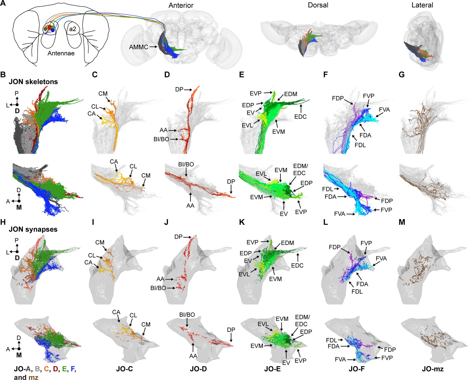
EM-based reconstruction of JONs.
(A) JON projections from the second antennal segment (a2) into the AMMC brain region (brain neuropile shown in gray). Anterior, dorsal, and lateral views of reconstructed JONs are shown. (B–G) Reconstructed JONs are shown from dorsal (top) and medial (bottom) views. (H–M) Dorsal (top) and medial (bottom) views of the JON pre- and post-synaptic sites are shown (colored dots) with a gray mesh that outlines the entire reconstructed JON population. See Figure 1—figure supplement 2 for pre- versus post-synaptic site distributions. All reconstructed JONs are shown in (B–G), but only fully reconstructed JONs are shown in (H–M) (JO-A and -B synapses not shown). JO-A and -B neurons were previously reconstructed by Kim et al., 2020. Colors in (A, B, and H) correspond to the zones to which the different JONs project, including zones A (dark gray), B (light gray), C (orange), D (red), E (green), F (blue), and mz (brown). Panels (C–G) and (I–M) show JONs that project specifically to zones C (C,I), D (D,J), E (E,K), F (F,L), or multiple zones (mz) (G,M). Color shades in (C–G) and (I–M) indicate different JON types that project to that zone. Zone subareas are indicated with labeled arrows. See Video 1 for 3D overview.
Figure 1—figure supplement 1
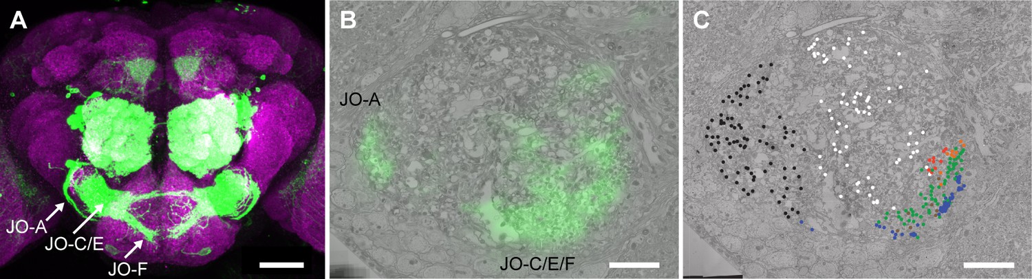
Identifying JONs in the EM volume.
(A) Brain of R27H08-GAL4 expressing GFP. Shown is the maximum intensity projection of anti-GFP (green) and anti-Bruchpilot (magenta) immunostaining to visualize the JON afferent GFP-labeled projections into the Bruchpilot-labeled brain neuropile. Scale bar, 100 μm. (B) Registration of R27H08-GAL4 expression pattern into the EM volume to locate JONs implicated in antennal grooming. Shown is an EM section of the point where the antennal nerve enters the brain. The labels indicate the GFP-highlighted regions that include either JO-A or -C, -E, and -F neurons. Scale bar, 10 μm. (C) Reconstruction of JONs in the medial region highlighted by the R27H08-GAL4 expression pattern. Colored dots indicate individual reconstructed JONs that were identified as JO-A (black), -B (white), -C (orange), -D (red), -E (green), -F (blue) neurons, and JONs that projected to multiple zones (brown). Scale bar, 10 μm.
Figure 1—figure supplement 2
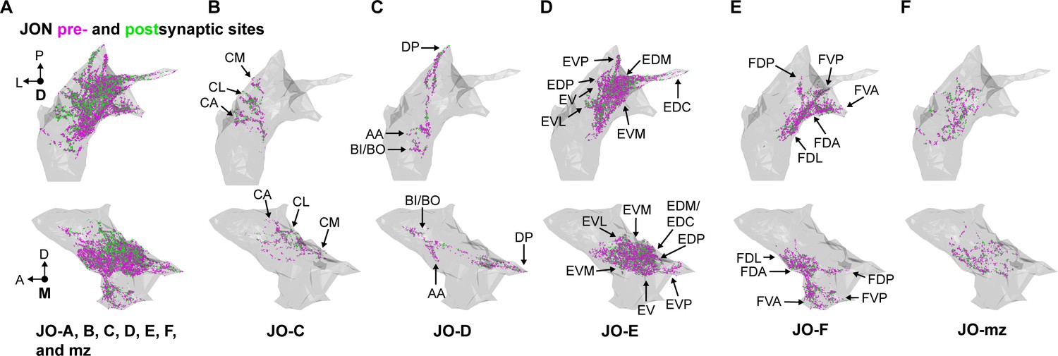
Distribution of JON synapses.
(A–F) Shown are the dorsal (top) and medial (bottom) views of the JON synapses, subdivided into pre- (magenta) and post-synaptic (green) sites. All synapses of completely reconstructed JONs are shown in (A). Synapses of zone C, D, E, F, or multiple zone (mz)-projecting JONs are shown in (B), (C), (D), (E), and (F), respectively. Zone subareas are indicated with labeled arrows.
Figure 2 with 7 supplements
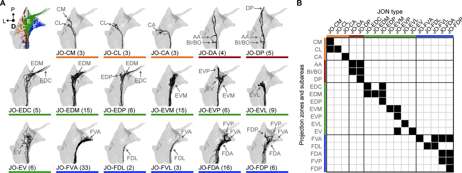
Specific JON types and their contributions to the JO topographical map.
(A) Dorsal views of the reconstructed JONs grouped by type. For each panel, a gray mesh outlines the entire reconstructed JON population. The top left panel shows all of the reconstructed JONs colored based on their projection zones, including zones C (orange), D (red), E (green), and F (blue). The remaining panels show each JON type in black. The number of JONs shown for each type is indicated below each panel. Subareas that receive projections from each JON type are indicated with labeled arrows. Individual reconstructed JONs for each type are shown in Figure 2—figure supplement 1, Figure 2—figure supplement 2, Figure 2—figure supplement 3, and Figure 2—figure supplement 4. Note that the JO-mz neurons are not shown because they could not be categorized into types. (B) Grid showing the projection zones and subareas of each JON type. Zone subareas that receive projections from each JON type are indicated with black squares. Colored lines indicate the zone for each subarea and each JON type (same color scheme used in A).
Figure 2—figure supplement 1
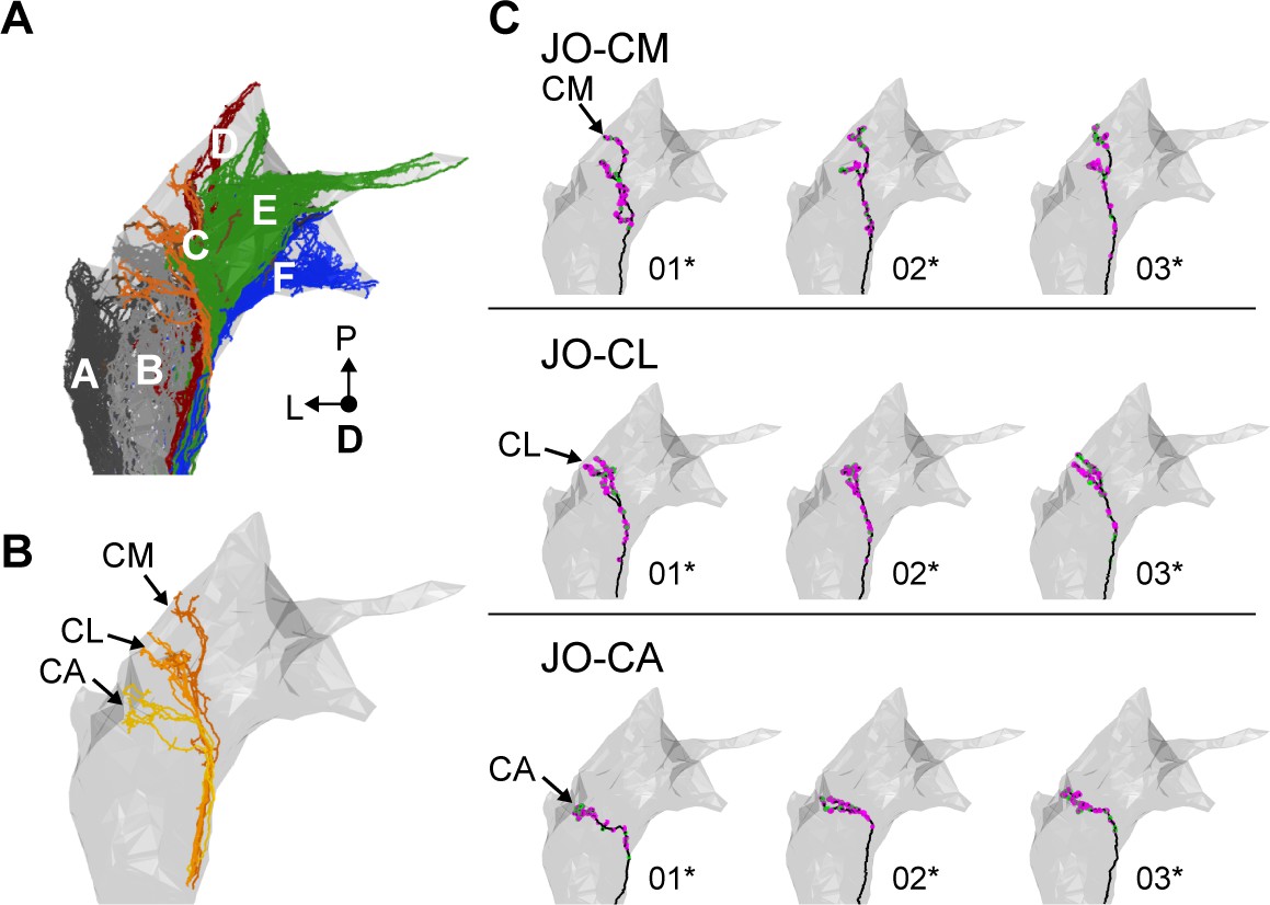
Individual reconstructed zone C-projecting JONs.
(A) Dorsal view of all reconstructed JONs from the EM dataset with the mesh that outlines the JON neuropile. The colors correspond to the zones to which the different JONs project, including zones A (dark gray), B (gray), C (orange), D (red), E (green), F (blue), and multiple zones (brown). (B) Dorsal view of all reconstructed JONs that project to zone C. Zone subareas are indicated with labeled arrows. (C) Dorsal views of individual zone C-projecting JON types. The JON type is labeled for each row. The subarea that receives the largest JON branch is labeled for each type. Numbers below each mesh indicate the corresponding reconstructed neuron in the EM dataset (e.g. JO_CM_01). Asterisks by the numbers indicate JONs that have been completely reconstructed, including pre- (magenta) and post-synaptic (green) sites.
Figure 2—figure supplement 2
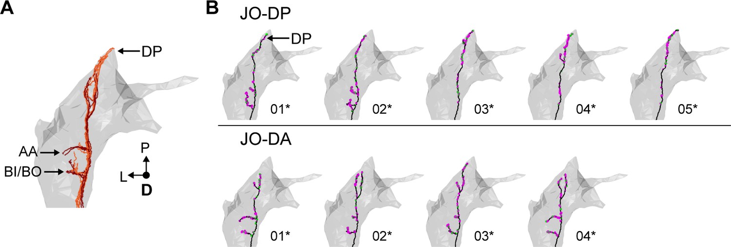
Individual reconstructed zone D-projecting JONs.
(A) Dorsal view of all reconstructed JONs that project to zone D. Zone subareas are indicated with labeled arrows. (B) Dorsal views of individual zone D-projecting JON types. The JON type is labeled for each row. Numbers below each mesh indicate the corresponding reconstructed neuron in the EM dataset (e.g. JO_DP_01). Asterisks by the numbers indicate JONs that have been completely reconstructed, including pre- (magenta) and post-synaptic (green) sites.
Figure 2—figure supplement 3
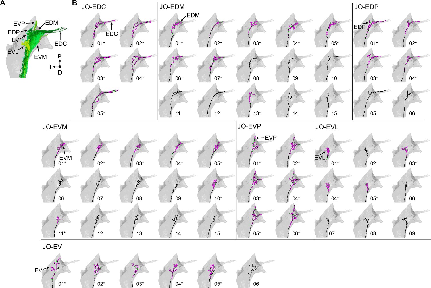
Individual reconstructed zone E-projecting JONs.
(A) Dorsal view of the reconstructed JONs that project to zone E. Zone subareas are indicated with labeled arrows. (B) Dorsal view of individual zone E-projecting JON types. Arrows with labels indicate the subarea that the JON projects to that led to the naming of the JON. The names of each of the seven JON types are labeled. Numbers below each mesh indicate the corresponding reconstructed neuron in the EM dataset (e.g. JO_EVM_01 or JO_EDP_05). Asterisks by the numbers indicate JONs that have been completely reconstructed, including pre- (magenta) and post-synaptic (green) sites.
Figure 2—figure supplement 4
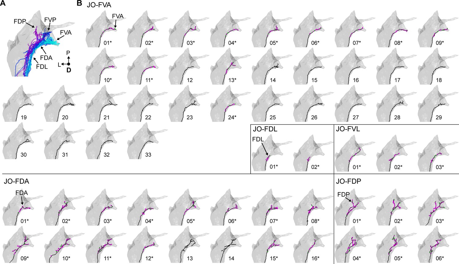
Individual reconstructed zone F-projecting JONs.
(A) Dorsal view of the reconstructed JONs that project to zone F. Zone subareas are indicated with labeled arrows. (B) Five different types of zone F-projecting JONs are shown from a dorsal view. The name of each of the five JON types is labeled. Arrows with labels indicate the subarea that the JON projects to that led to the naming of the JON. Numbers below each mesh indicate the corresponding reconstructed neuron in the EM dataset (e.g. JO_FVA_01 or JO_FDA_02). Asterisks by the numbers indicate JONs that have been completely reconstructed, including pre- (magenta) and post-synaptic (green) sites.
Figure 2—figure supplement 5

Individual reconstructed multiple zone-projecting JONs.
(A) Dorsal view of the reconstructed JONs that project to multiple zones. (B) Dorsal view of individual JO-mz neurons. Numbers below each mesh indicate the corresponding reconstructed neuron in the EM dataset (e.g. JO_mz_01). Asterisks by the numbers indicate JONs that have been completely reconstructed, including pre- (magenta) and post-synaptic (green) sites.
Figure 2—figure supplement 6
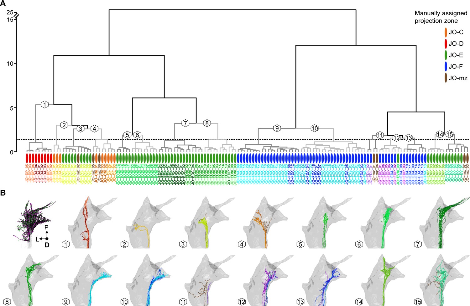
Correspondence between manual annotation and NBLAST clustering in the categorization of JONs.
(A) Dendrogram of hierarchically clustered scores from an NBLAST query of 147 reconstructed JONs. Oval colors indicate the manual assignment of each JON as projecting to a specific zone. Colors of specific neuron names indicate the manually annotated neuron types (e.g. JO-FVA in cyan, JO-FDA in dark blue). Branch numbers indicate JON groups that are shown in (B) resulting from a cut height of 1.4 (dotted line). (B) NBLAST-clustered JON groups (15 groups at h = 1.4). Neuron colors indicate manually annotated neuron types and correspond to the neuron type names in (A). The first panel shows how the JONs were pruned for NBLAST analysis to include only synapse-bearing parts of the neurons (JON parts used for NBLAST analysis shown in black, see Materials and methods for details) with pre- and post-synaptic sites in magenta and green respectively.
Figure 2—figure supplement 7
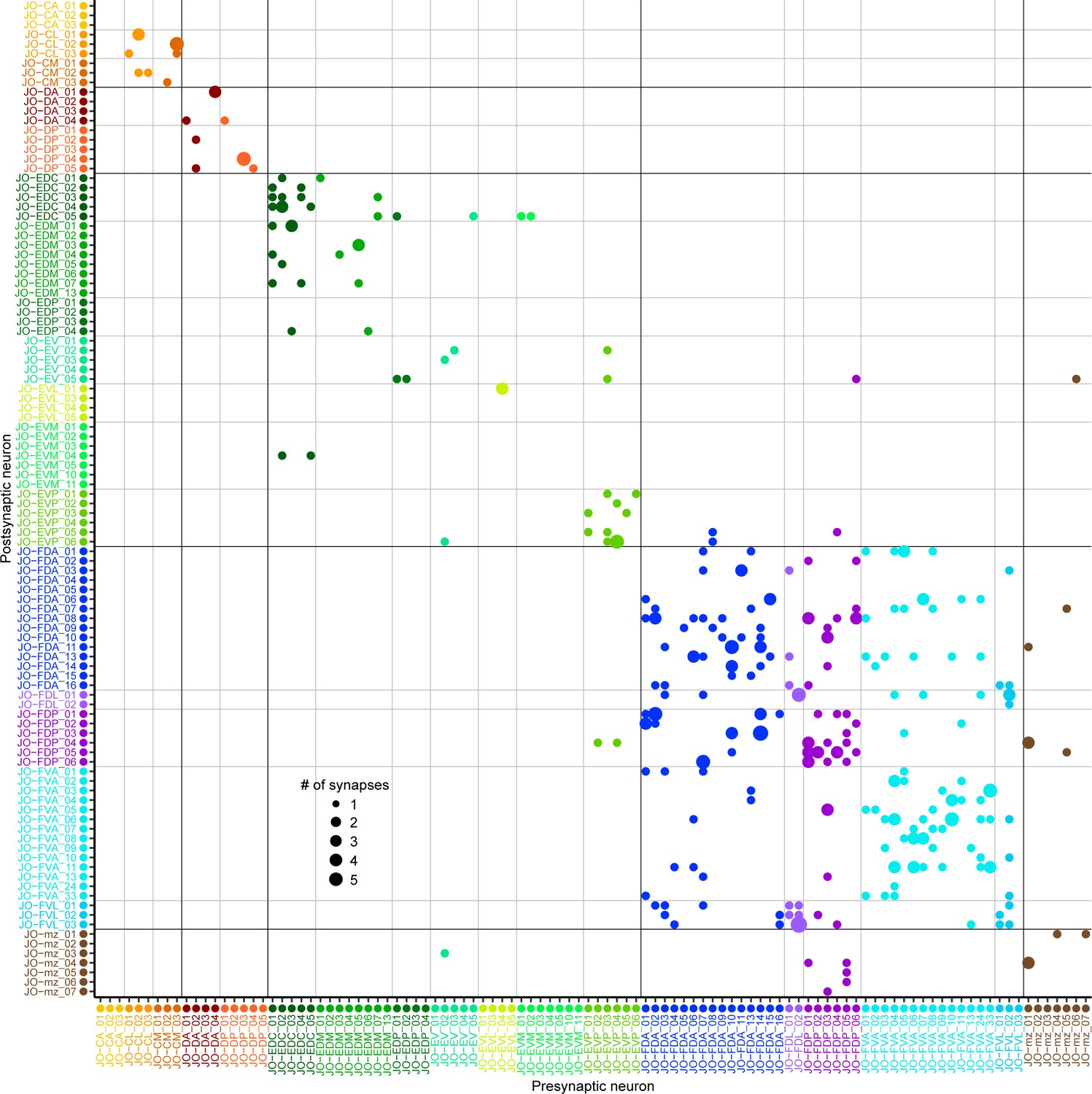
JON-to-JON synaptic connectivity.
Plotted is a matrix of the axo-axonic synaptic connections of the completely reconstructed JONs from this study (presynaptic neurons – x axis, post-synaptic – y axis). The different sized dots on the grid indicate the strength (# of synapses) for each connection. Synapse strength reference dots are shown in the bottom left quadrant. The matrix shows the synaptic connections among the JO-C (orange), -E (green), -F (blue), and -mz (brown) neurons. For the synapse numbers for each connection, see Supplementary file 2.
Figure 3 with 2 supplements
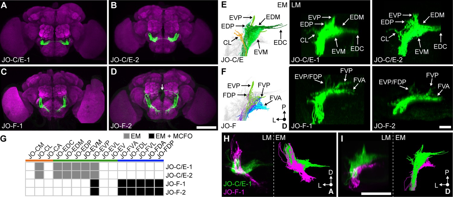
Driver lines that express in JO-C/E or JO-F neurons.
(A–D) Shown are maximum intensity projections of brains (anterior view) in which driver lines JO-C/E-1 (A), JO-C/E-2 (B), JO-F-1 (C), and JO-F-2 (D) drive expression of green fluorescent protein (mCD8::GFP). Brains were immunostained for GFP (green) and Bruchpilot (magenta). The arrow shown in (D) indicates a neuron that is not a JON. Scale bar, 100 μm. Figure 3—figure supplement 1 shows the ventral nerve cord expression pattern for each line. (E, F) Dorsal view of EM-reconstructed JON types (left panels) that are predicted to be in the expression patterns of the confocal light-microscopy (LM) images of driver-labeled neurons (middle and right panels). Driver line expression patterns of JO-C/E-1 (middle) and −2 (right) shown in (E) and JO-F-1 (middle) and −2 (right) shown in (F). Subareas are indicated with arrows. Note that in (F) the subareas FDL and FDA are not labeled because they are not visible in the dorsal view. Scale bar, 20 μm. (G) Table of JON types that are predicted to be in each driver expression pattern. The shading of each box indicates whether the predictions are supported by EM reconstructions alone (gray), or by EM and MCFO data (black). MCFO data is shown in Figure 3—figure supplement 2. (H, I) Computationally aligned expression patterns of JO-C/E-1 (green) and JO-F-1 (magenta) from anterior (H) and dorsal (I) views (left panels) in comparison with the EM-reconstructed JONs (right panels). Scale bar, 50 μm.
Figure 3—figure supplement 1
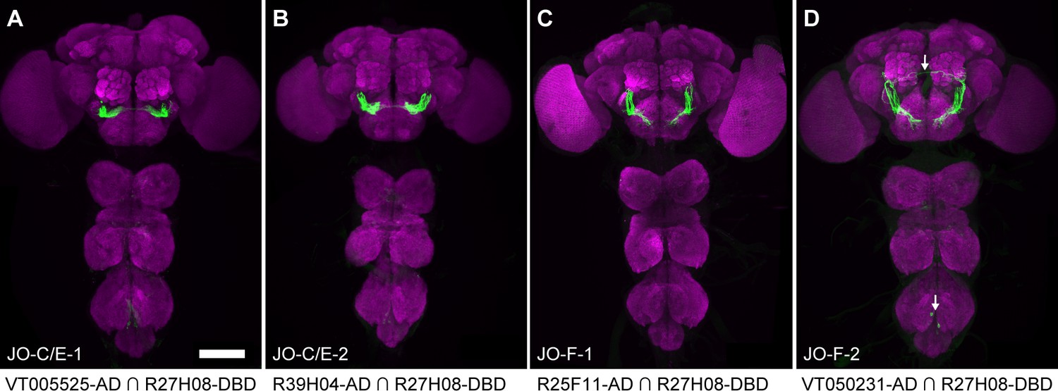
Driver lines that express in JO-C/E or -F neurons.
(A–D) Driver lines that express GFP in subpopulations of JONs. Shown are the brains and ventral nerve cords of JO-C/E-1 (A), JO-C/E-2 (B), JO-F-1 (C), and JO-F-2 (D). Images are maximum intensity projections of CNSs immunostained for GFP (green) and Bruchpilot (magenta). The arrows in (D) indicate neurons that are not JONs. Scale bar, 100 μm.
Figure 3—figure supplement 2
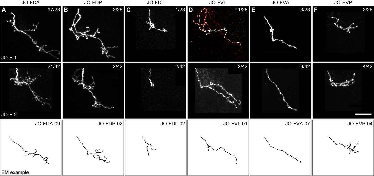
Stochastic labeling of individual JONs in the JO-F-1 and JO-F-2 expression patterns.
(A–F) Anterior view of different MCFO-labeled JON types in the expression patterns of JO-F-1 (top) and JO-F-2 (middle). Shown are maximum intensity projections of each JON expressing a tagged protein that is stained using a tag-specific antibody (see Materials and methods for information about the tagged protein and antibodies used). Top right corner of each panel indicates the number of JONs that were labeled for each type versus the total MCFO-labeled JONs that we obtained (white neurons are the type indicated). Note that the number of individual labeled JONs does not add up to the total number of MCFO-labeled JONs (27 out of 28 for JO-F-1 and 39 out of 42 for JO-F-2). The additional neurons were not included in the analysis because they had ambiguous morphology that could not be definitively linked to a particular JON type. Bottom panels show EM-reconstructed examples of each neuron type (neuron names are indicated in the top right corner). The JON types are JO-FDA (A), -FDP (B), -FDL (C), -FVL (D), -FVA (E), and -EVP (F). Scale bar, 20 μm.
Figure 4
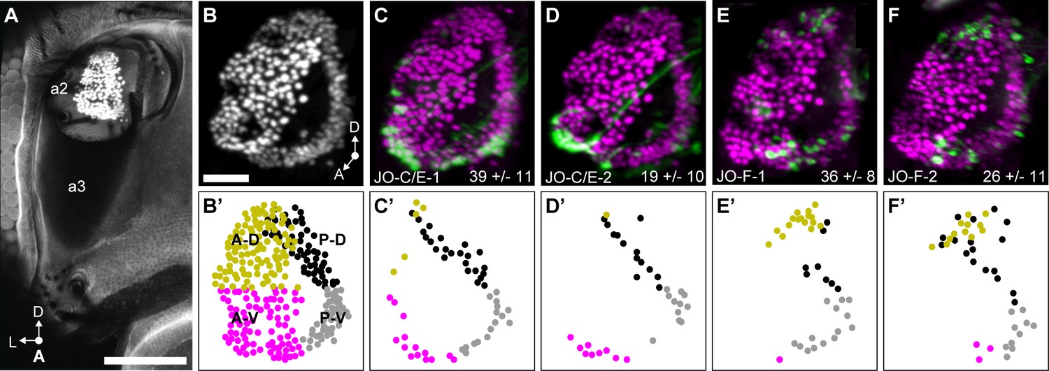
JO chordotonal organ distribution of JONs that are targeted by JO-C/E and F driver lines.
(A) Anterior view of the antennal region of the head with the JON nuclei labeled with an anti-ELAV antibody in the second antennal segment (labeled a2, third segment is labeled a3). A maximum intensity projection is shown. The head is visualized as autofluorescence from the cuticle. Scale bar, 100 μm. (B) JON nuclei laterally rotated about the ventral/dorsal axis (~40°). Scale bar, 25 μm. (C–F) Driver lines expressing GFP in the JO. Shown is immunostaining of GFP (green) and ELAV (magenta). The average number of JONs labeled in each line ±the standard deviation is shown in the bottom right corner. (B’) Anterior view of manually labeled JON cell bodies in different regions from the confocal stack shown in (B) (not laterally rotated like in (B–F), ~60% JON cell bodies labeled). The JO regions are color coded, including anterior-dorsal (A-D, mustard), posterior-dorsal (P-D, black), anterior-ventral (A-V, magenta), and posterior-ventral (P-V, gray). (C’–F’) Manually labeled JON cell bodies (dots) that expressed GFP in a confocal z-stack of each driver line. This highlights GFP-labeled JONs in the posterior JO that are difficult to view in the maximum projections shown in (C–F). The colors indicate the JO region where the cell body is located. Shown are JO-C/E-1 (C,C’), JO-C/E-2 (D,D’), JO-F-1 (E,E’), and JO-F-2 (F,F’).
Figure 5 with 2 supplements
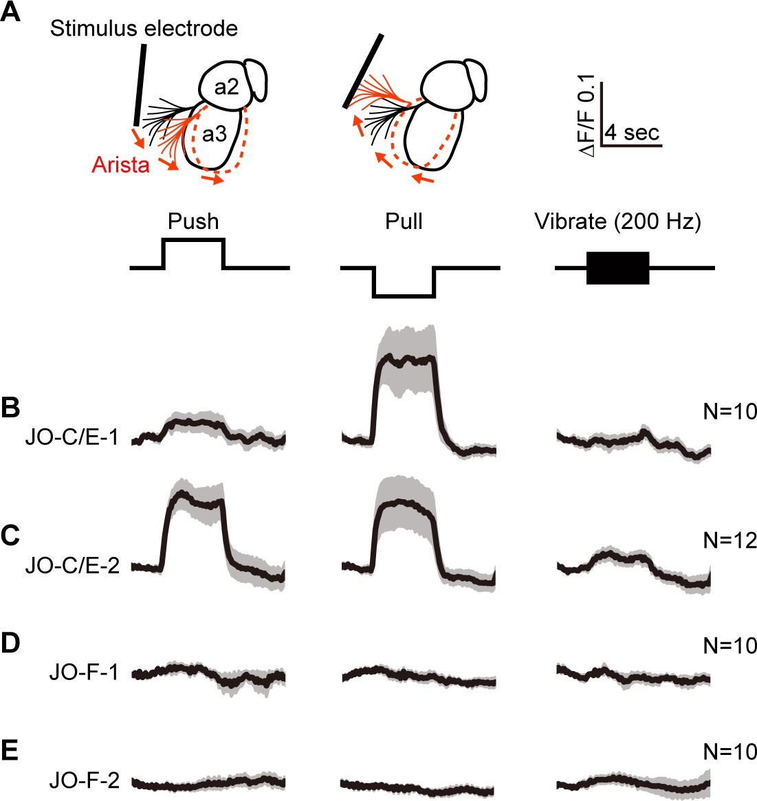
Testing the responses of JO-C/E and JO-F neurons to stimulations of the antennae.
(A) Schematic lateral view of a fly antenna. An electrostatically charged electrode pushes or pulls the antenna via the arista towards or away from the head, respectively, or induces a 200 Hz sinusoid. (B–E) Calcium response of JONs to stimulations of the antennae. Flies were attached to an imaging plate, dorsal side up. The proboscis was removed to access the ventral brain for imaging GCaMP6f fluorescence changes (ΔF/F) in the JON afferents. Stimulations of the antennae were delivered for 4 s as indicated above the traces. 10 or 12 flies were tested for each driver line (N = number of flies tested). For each fly, four trials were run for each stimulus and then averaged. Each row shows the mean trace of all flies tested (black lines) from a different driver line expressing GCaMP6f, including JO-C/E-1 (B), JO-C/E-2 (C), JO-F-1 (D), JO-F-2 (E). The gray envelopes indicate the standard error of the mean. See Figure 5—figure supplement 1 and Figure 5—figure supplement 2 for statistical analysis.
Figure 5—figure supplement 1
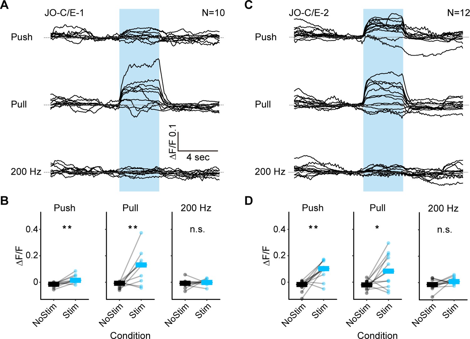
Responses of the JO-C/E neurons to mechanical stimuli: individual traces and statistical analysis.
(A–D) GCaMP6f was expressed in either JO-C/E-1 (A,B) or JO-C/E-2 (C,D). (A,C) Shown are the GCaMP6f fluorescence traces of individual flies while different mechanosensory stimulations were delivered. Each trace represents the mean of four trials for each fly. The stimulus duration was 4 s and is indicated with blue boxes. 10 or 12 flies were tested for each driver line (N = number of flies tested). The mean traces of all the tested flies are shown in Figure 5B,C. (B,D) Plots of the measured fluorescence before and during each stimulus (NoStim and Stim, respectively) for the mean value of four trials for each fly (dots), and the median value of all flies (bars). The Wilcoxon signed-rank test was used for each condition (asterisks indicate *p<0.05, **p<0.001).
Figure 5—figure supplement 2
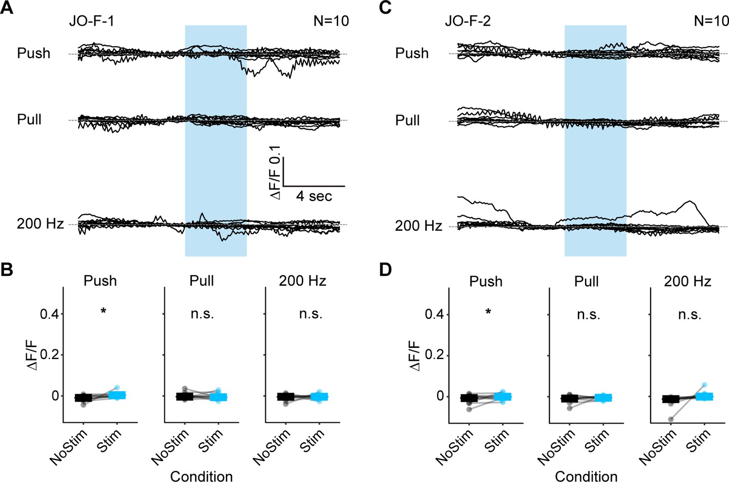
Responses of the JO-F neurons to mechanical stimuli: individual traces and statistical analysis.
(A–D) GCaMP6f was expressed in either JO-F-1 (A,B) or JO-F-2 (C,D). (A,C) Shown are the GCaMP6f fluorescence traces of individual flies while different mechanosensory stimulations were delivered. Each trace represents the mean of four trials for each fly. The stimulus duration was 4 s and is indicated with blue boxes. 10 flies were tested for each driver line (N = number of flies tested). The mean traces of all the tested flies are shown in Figure 5D,E. (B,D) Plots of the measured fluorescence before and during each stimulus (NoStim and Stim, respectively) for the mean value of four trials for each fly (dots), and the median value of all flies (bars). The Wilcoxon signed-rank test was used for each condition (asterisks indicate *p<0.05).
Figure 6 with 1 supplement
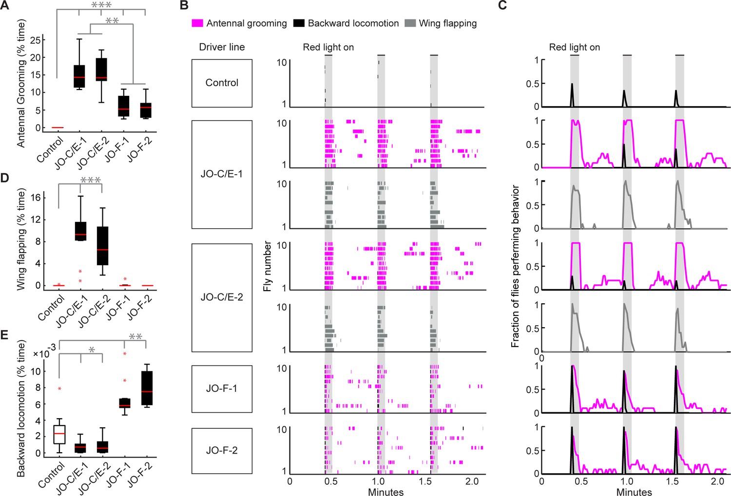
Optogenetic activation of JO-C/E or JO-F neurons elicits common and distinct behavioral responses.
(A, D, E) Percent time flies spent performing antennal grooming (A), wing flapping (D), or backward locomotion (E) with optogenetic activation of JONs targeted by JO-C/E-1, JO-C/E-2, JO-F-1, and JO-F-2. Control flies do not express CsChrimson in JONs. Bottom and top of the boxes indicate the first and third quartiles respectively; median is the red line; whiskers show the upper and lower 1.5 IQR; red dots are data outliers. N ≥ 10 flies for each box; asterisks indicate *p<0.05, **p<0.001, ***p<0.0001, Kruskal–Wallis and post-hoc Mann–Whitney U pairwise tests with Bonferroni correction. Figure 6—source data 1 contains numerical data used for producing each box plot. (B) Ethograms of manually scored videos show the behaviors elicited with red-light induced optogenetic activation. Ethograms of individual flies are stacked on top of each other. The behaviors performed are indicated in different colors, including antennal grooming (magenta), wing flapping (gray), and backward locomotion (black). Light gray bars indicate the period where a red-light stimulus was delivered (5 s). (C) Histograms show the fraction of flies that performed each behavior in one-second time bins. Note that only JO-C/E-1 and −2 elicited wing flapping, which was not mutually exclusive with grooming. Therefore, an extra row of wing flapping ethograms and histograms is shown for those lines. See Video 2, Video 3, and Video 4 for representative examples.
-
Figure 6—source data 1
Numerical data used for box plots.
Data used for producing box plots shown in Figure 6A,D,E.
- https://cdn.elifesciences.org/articles/59976/elife-59976-fig6-data1-v2.csv.zip
Figure 6—figure supplement 1
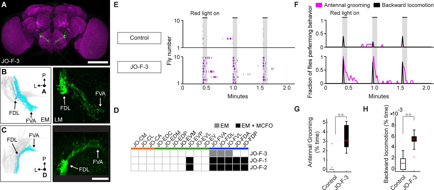
Driver line that expresses in JO-F neurons.
(A) Shown is a maximum intensity projection of a brain (anterior view) of JO-F-3 (R60E02-LexA) expressing green fluorescent protein (myr::GFP) immunostained for GFP (green) and Bruchpilot (magenta). Scale bar, 100 μm. (B,C) Anterior (B) and dorsal (C) views of EM-reconstructed JO-F neuron types (left panels) that are predicted to be in the expression pattern of JO-F-3 (right panels). Subareas are indicated with arrows. Scale bar, 20 μm. (D) Table of JON types that are proposed to be in the JO-F-3 expression pattern, compared with JO-F-1 and −2. The shade of each box indicates whether the predictions are supported by EM reconstructions alone (gray), or by EM and MCFO data (black). (E,F) Ethograms (E) and histograms (F) of manually scored video show the behaviors elicited with red-light induced optogenetic activation. Ethograms and histograms are shown as described in Figure 6. (G,H) Percent time flies spent performing antennal grooming (G) or backward locomotion (H) with optogenetic activation of JONs targeted by JO-F-3. Box plots are shown as described in Figure 6.
Videos
Video 1
EM-reconstructed JONs.
Shown are the different JON types for each subpopulation.
Video 2
Optogenetic activation of JO-C/E neurons elicits antennal grooming and wing flapping.
CsChrimson was expressed in JO-C/E neurons using the JO-C/E-2 driver line. The infrared light in the bottom right corner indicates when the red light was on to activate the JO-C/E neurons.
Video 3
Optogenetic activation of JO-F neurons elicits antennal grooming and backward locomotion.
CsChrimson was expressed in JO-F neurons using the JO-F-2 driver line. The infrared light in the bottom right corner indicates when the red light was on to activate the JO-F neurons.
Video 4
Optogenetic stimulus induces backward locomotion in control flies.
Tables
Key resources table
| Reagent type (species) or resource | Designation | Source or reference | Identifiers | Additional information |
|---|---|---|---|---|
| Genetic reagent (D. melanogaster) | R27H08-GAL4 | Jenett et al., 2012 | RRID:BDSC_49441 | |
| Genetic reagent (D. melanogaster) | R27H08-DBD | Dionne et al., 2017 | RRID:BDSC_69106 | |
| Genetic reagent (D. melanogaster) | VT005525-AD | Tirián and Dickson, 2017 | RRID:BDSC_72267 | aka 100C03 |
| Genetic reagent (D. melanogaster) | R39H04-AD | Dionne et al., 2017 | RRID:BDSC_75734 | |
| Genetic reagent (D. melanogaster) | R25F11-AD | Dionne et al., 2017 | RRID:BDSC_70623 | |
| Genetic reagent (D. melanogaster) | VT050231-AD | Tirián and Dickson, 2017 | RRID:BDSC_71886 | aka 122A08 |
| Genetic reagent (D. melanogaster) | JO-C/E-1 | This paper | Stock contains VT005525-AD and R27H08-DBD | |
| Genetic reagent (D. melanogaster) | JO-C/E-2 | This paper | Stock contains R39H04-AD and R27H08-DBD | |
| Genetic reagent (D. melanogaster) | JO-F-1 | This paper | Stock contains R25F11-AD and R27H08-DBD | |
| Genetic reagent (D. melanogaster) | JO-F-2 | This paper | Stock contains VT050231-AD and R27H08-DBD | |
| Genetic reagent (D. melanogaster) | BPADZp; BPZpGDBD | Hampel et al., 2015 | RRID:BDSC_79603 | spGAL4 control |
| Genetic reagent (D. melanogaster) | JO-F-3 (R60E06-LexA) | Pfeiffer et al., 2010 | RRID:BDSC_54905 | |
| Genetic reagent (D. melanogaster) | BDPLexA | Pfeiffer et al., 2010 | RRID:BDSC_77691 | |
| Genetic reagent (D. melanogaster) | 10XUAS-IVS-mCD8::GFP | Pfeiffer et al., 2010 | RRID:BDSC_32185 | |
| Genetic reagent (D. melanogaster) | 20XUAS-IVS-CsChrimson-mVenus | Klapoetke et al., 2014 | RRID:BDSC_55134 | |
| Genetic reagent (D. melanogaster) | 13XLexAop2-IVS-myr::GFP | RRID:BDSC_32209 | ||
| Genetic reagent (D. melanogaster) | MCFO-5 | Nern et al., 2015 | RRID:BDSC_64089 | |
| Genetic reagent (D. melanogaster) | 20XUAS-IVS-GCaMP6f | RRID:BDSC_42747 | ||
| Genetic reagent (D. melanogaster) | 13XLexAop2-IVS-CsChrimson-mVenus | RRID:BDSC_55137 | ||
| Antibody | anti-GFP (Rabbit polyclonal) | Thermo Fisher Scientific | Cat# A-11122, RRID:AB_221569 | IF(1:500) |
| Antibody | anti-Brp (Mouse monoclonal) | DSHB | Cat# nc82, RRID:AB_2314866 | IF(1:50) |
| Antibody | anti-ELAV (Mouse monoclonal) | DSHB | Cat# Elav-9F8A9, RRID:AB_528217 | IF(1:50) |
| Antibody | anti-ELAV (Rat monoclonal) | DSHB | Cat# Rat-Elav-7E8A10 anti-elav, RRID:AB_528218 | IF(1:50) |
| Antibody | anti-FLAG (Rat monoclonal) | Novus Biologicals | Cat# NBP1-06712, RRID:AB_1625981 | IF(1:300) |
| Antibody | anti-HA (Rabbit monoclonal) | Cell Signaling Technology | Cat# 3724, RRID:AB_1549585 | IF(1:500) |
| Antibody | anti-V5 (Mouse monoclonal) | BIO-RAD | Cat# MCA1360, RRID:AB_322378 | IF(1:300) |
| Antibody | anti-Rabbit AF488 (Goat polyclonal) | Thermo Fisher Scientific | Cat# A-11034, RRID:AB_2576217 | IF(1:500) |
| Antibody | anti-Mouse AF568 (Goat polyclonal) | Thermo Fisher Scientific | Cat# A-11031, RRID:AB_144696 | IF(1:500) |
| Antibody | anti-Rat AF568 (Goat polyclonal) | Thermo Fisher Scientific | Cat# A-11077, RRID:AB_2534121 | IF(1:500) |
| Antibody | anti-Rat AF633 (Goat polyclonal) | Thermo Fisher Scientific | Cat# A-21094, RRID:AB_2535749 | IF(1:500) |
| Chemical compound, drug | Paraformaldehyde 20% | Electron Microscopy Sciences | Cat# 15713 | |
| Chemical compound, drug | all-trans-Retinal | Toronto Research Chemicals | Cat# R240000 | |
| Software, algorithm | Vcode | Hagedorn et al., 2008 | http://social.cs.uiuc.edu/projects/vcode.html | |
| Software, algorithm | Fiji | Schindelin et al., 2012 | http://fiji.sc/ | |
| Software, algorithm | R | https://www.r-project.org/ | ||
| Software, algorithm | CMTK | Jefferis et al., 2007 | https://www.nitrc.org/projects/cmtk/ | |
| Software, algorithm | FluoRender | Wan et al., 2012 | http://www.sci.utah.edu/software/fluorender.html | |
| Software, algorithm | Blender version 2.79 | https://www.blender.org/download/releases/2-79/ | ||
| Software, algorithm | CATMAID | Schneider-Mizell et al., 2016 | https://catmaid.readthedocs.io/en/stable/ | |
| Software, algorithm | MATLAB | MathWorks Inc, Natick, MA | ||
| Software, algorithm | natverse | Bates et al., 2020 | http://natverse.org/ | |
| Software, algorithm | CATMAID-to-Blender plugin | Schlegel et al., 2016 | https://github.com/schlegelp/CATMAID-to-Blender |
Additional files
-
Supplementary file 1
Detailed information about the EM-reconstructed JONs.
Includes the JON FAFB skeleton ID numbers, raw and smooth cable length, number of nodes, number of pre- and post-synaptic sites, and NBLAST group numbers.
- https://cdn.elifesciences.org/articles/59976/elife-59976-supp1-v2.csv.zip
-
Supplementary file 2
JON all-to-all connectivity matrix.
Shows the number of synapses for each JON-to-JON connection (presynaptic neurons – rows, post-synaptic – columns).
- https://cdn.elifesciences.org/articles/59976/elife-59976-supp2-v2.csv.zip
-
Transparent reporting form
- https://cdn.elifesciences.org/articles/59976/elife-59976-transrepform-v2.docx
Download links
A two-part list of links to download the article, or parts of the article, in various formats.
Downloads (link to download the article as PDF)
Open citations (links to open the citations from this article in various online reference manager services)
Cite this article (links to download the citations from this article in formats compatible with various reference manager tools)
Distinct subpopulations of mechanosensory chordotonal organ neurons elicit grooming of the fruit fly antennae
eLife 9:e59976.
https://doi.org/10.7554/eLife.59976


