Visual attention modulates the integration of goal-relevant evidence and not value
- Institute of Cognitive Neuroscience, University College London, United Kingdom
- School of Psychological Sciences and Sagol School of Neuroscience, Tel Aviv University, Israel
- Department of Economics and Woodrow Wilson School, Princeton University, United States
- Wellcome Centre for Human Neuroimaging, University College London, United Kingdom
Figures
Figure 1
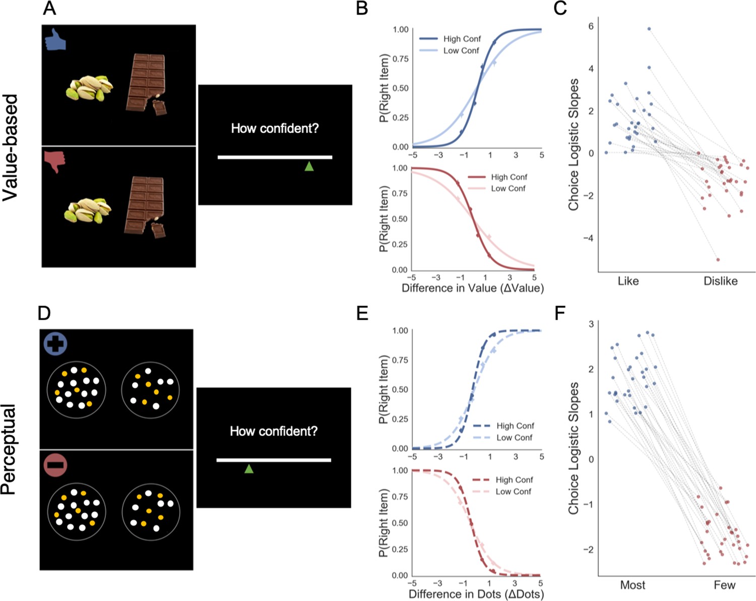
Task and behavioural results.
Value-based decision task (A). Participants choose between two food items presented in an eye-contingent way. Before the choice stage, participants reported the amount of money they were willing to bid to eat that snack. In the like frame (top) participants select the item they want to consume at the end of the experiment. In the dislike frame (bottom) participants choose the opposite, the item they would prefer to avoid. After each choice participants reported their level of confidence. (B) After a median split for choice confidence, a logistic regression was calculated for the probability of choosing the right-hand item depending on the difference in value (ValueRight– ValueLeft) for like (top) and dislike (bottom) framing conditions. The logistic curve calculated from the high confidence trials is steeper, indicating an increase in accuracy. (C) Slope of logistic regressions predicting choice for each participant, depending on the frame. The shift in sign of the slope indicates that participants are correctly modifying their choices depending on the frame. Perceptual decision task (D) Participants have to choose between two circles containing dots, also presented eye-contingently. In the most frame (top), participants select the circle with more white dots. In the fewest frame (bottom), they choose the circle with the lower number of white dots. Distractor dots (orange) are included in both frames to increase the difficulty of the task. Confidence is reported at the end of each choice. We obtained a similar pattern of results to the one observed in the Value Experiments in terms of probability of choice (E) and the flip in the slope of the choice logistic model between most and fewest frames (F).
Figure 2
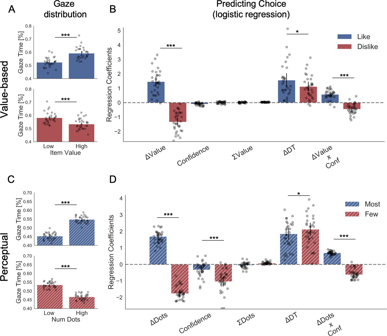
Attention and choice in Value and Perceptual Experiments.
(A) Gaze allocation time depends on the frame: while visual fixations in the like frame go preferentially to the item with higher value (top), during the dislike frame participants look for longer at the item with lower value (bottom). Dots in the bar plot indicate participants’ average gaze time across trials for high and low value items. Time is expressed as the percentage of trial time spent looking at the item. Similar results were found for gaze distribution in the Perceptual Experiment (C) participants gaze the circle with higher number of dots in most frame and the circle with lower number of dots in fewest frame. Hierarchical logistic modelling of choice (probability of choosing right item) in Value (B) and Perceptual (D) Experiments, shows that participants looked for longer (ΔDT) at the item they chose in both frames. All predictors are z-scored at the participant level. In both regression plots, bars depict the fixed-effects and dots the mixed-effects of the regression. Error bars show the 95% confidence interval for the fixed effect. In Value Experiment: ΔValue: difference in value between the two items (ValueRight– ValueLeft); RT: reaction time; ΣValue: summed value of both items; ΔDT: difference in dwell time (DTRight– DTLeft); Conf: confidence. In Perceptual Experiment: ΔDots: difference in dots between the two circles (DotsRight– DotsLeft); ΣDots: summed number of dots between both circles. ***p<0.001, **p<0.01, *p<0.05.
Figure 3

Fixation effects on the chosen item.
Last fixation effects: (A) in the Value Experiment, a logistic regression was calculated for the probability the last fixation is on the chosen items (P(LastFix = Chosen)) depending on the difference in value of the item last fixated upon and the alternative item. As reported in previous studies, in like frame, we find it is more probable that the item last fixated upon will be chosen when the value of that item is relatively higher. In line with the hypothesis that goal-relevant evidence, and not value, is being integrated to make the decision, during the dislike frame the effect shows the opposite pattern: P(LastFix = Chosen) is higher when the value of the item last fixated on is lower, that is, the item fixated on is more relevant given the frame. (B) A similar analysis in the Perceptual Experiment mirrors the results in the Value Experiment with a flip in the effect between most and fewest frames. Lines represent the model predictions and dots are the data binned across all participants. ΔValue and ΔDots measures are z-scored at the participant level. Gaze preference in time: (C) Pearson correlation between gaze position and difference in value (ΔValue) was calculated for each time point during the first 2 s of the trials. In the Value Experiment, after an initial phase of random exploration, fixations are positively correlated with the high value item in like frame, while this effect is the opposite for dislike frame, that is, fixations are directed to the low value item. (D) In the Perceptual Experiment, a similar pattern of goal-relevant fixations emerges. Lines in both figures correspond to the time point correlation considering all trials and participants. Shaded area corresponds to the standard error. Black line indicates time points with statistically significant difference between frames, resulting from a permutation test (p-value<0.01 for at least 6 time bins, 60 ms). Correction for multiple comparison was performed using FDR, α ≤ 0.01.
Figure 4
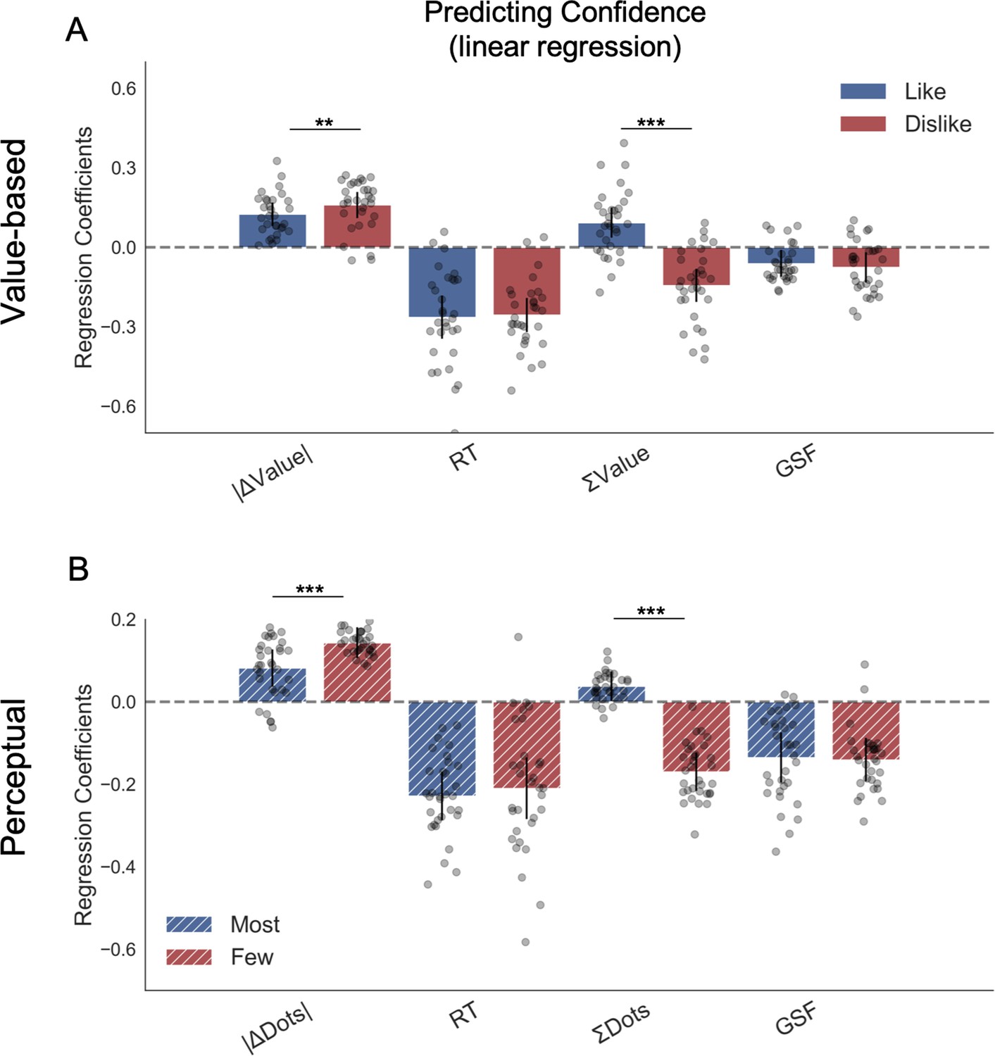
Hierarchical linear regression model to predict confidence.
(A) In Value Experiment, a flip in the effect of ΣValue over confidence in the dislike frame was found. (B) In Perceptual Experiment, a similar pattern was found in the effect of ΣDots over confidence in the fewest frame. The effect of the other predictors on confidence in both experiments and frames coincides with previous reports (Folke et al., 2017). All predictors are z-scored at the participant level. In both regression plots, bars depict the fixed-effects and dots the mixed-effects of the regression. Error bars show the 95% confidence interval for the fixed effect. In Value Experiment: ΔValue: difference in value between the two items (Valueright– Valueleft); RT: reaction time; ΣValue: summed value of both items; ΔDT: difference in dwell time (DTright– DTleft); GSF: gaze shift frequency; ΔDT: difference in dwell time. In Perceptual Experiment: ΔDots: difference in dots between the two circles (Dotsright– Dotsleft); ΣDots: summed number of dots between both circles. ***p<0.001, **p<0.01, *p<0.05.
Figure 5
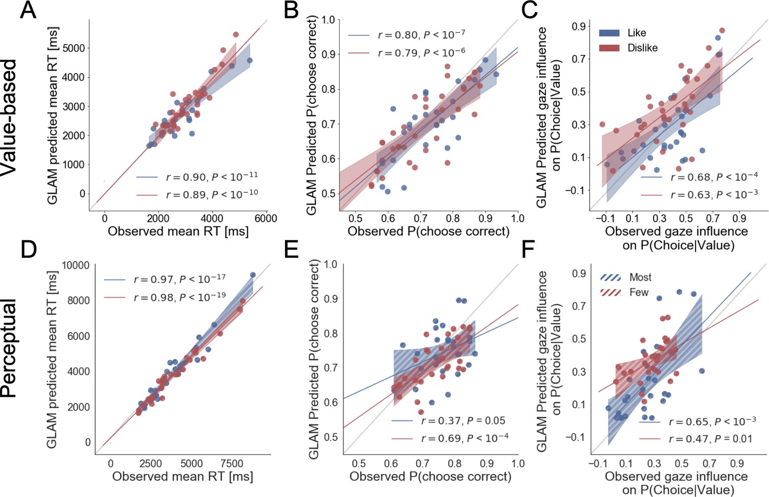
Individual out-of-sample GLAM predictions for behavioural measures in Value (A-C) and Perceptual Experiments (D–F).
In value-based decision, (A) the model predicts individuals mean RT; (B) the probability of choosing the item with higher value in like frame, and the item with lower value in dislike frame; and (C) the influence of gaze in choice probability. In the Perceptual Experiment, (D) the model also predicts RT and (F) gaze influence. (E) The model significantly predicts the probability of choosing the best alternative in the fewest frame only (in the most frame a trend was found). The results corresponding to the models fitted with like/most frame data are presented in blue, and with dislike/fewest frame data in red. Dots depict the average of observed and predicted measures for each participant. Lines depict the slope of the correlation between observations and the predictions. Mean 95% confidence intervals are represented by the shadowed region in blue or red, with full colour representing Value Experiment and striped colour Perceptual Experiment. All model predictions are simulated using parameters estimated from individual fits for even-numbered trials.
Figure 6
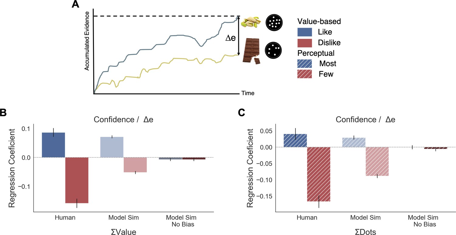
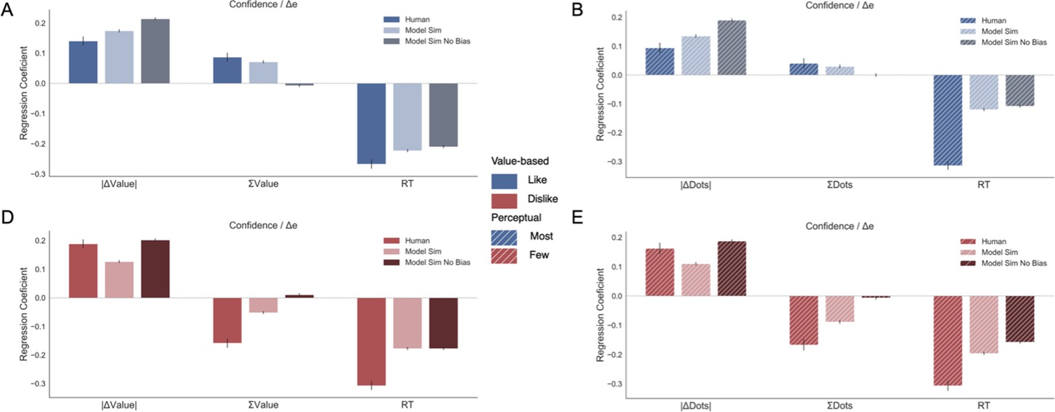
Balance of evidence (Δe) simulated with GLAM reproduces ΣValue and ΣDots effects over confidence.
(A) GLAM is a linear stochastic race model in which two alternatives accumulate evidence until a threshold is reached by one of them. Δe has been proposed as a proxy for confidence and it captures the difference in evidence available in both accumulators once the choice for that trial has been made. (B) Using Δe simulations, we captured the flip of the effect of ΣValue over confidence between like and dislike frames. Δe simulations were calculated using the model with parameters fitted for each individual participant. A pooled linear regression model was estimated to predict Δe. The effects of ΣValue predicting Δe are presented labelled as ’Model Sim’. A second set of simulations was generated using a model in which no asymmetries in gaze allocation were considered (i.e. no attentional biases). This second model was not capable of recovering ΣValue effect on Δe and is labelled as ’Model Sim No Bias’. ΣValue coefficients for a similar model using participants’ data predicting confidence are also presented labelled as ‘Human’ for comparison. (C) A similar pattern of results is found in the Perceptual Experiment, with the model including gaze bias being capable of recovering ΣDots effect on Δe. This novel effect may suggests that goal-relevant information is also influencing the generation of second-order processes, as confidence. This effect may be originated by the attentional modulation of the accumulation dynamics. Coloured bars show the parameter values for ΣValue and ΣDots and the error bars depict the standard error. Solid colour indicates the Value Experiment and striped colours indicate the Perceptual Experiment. All predictors are z-scored at participants level.
Appendix 1—figure 1
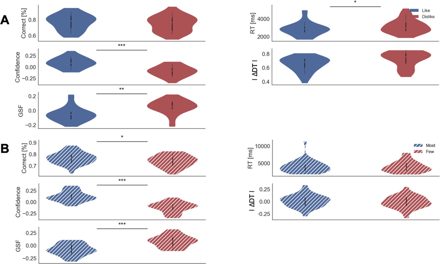
Behavioural results for Value (A) and Perceptual (B) Experiments.
Confidence, DDT, and GSF values have been z-scored per participant. In the violin plot, red and blue areas indicate the distribution of the parameters across participants. Black bars present the 25, 50, and 75 percentiles of the data. Solid colour indicates the Value Experiment and striped colours indicate the Perceptual Experiment. RT: reaction time; ∆DT: Difference in Dwell Time; GSF: Gaze Shift Frequency.
Appendix 1—figure 2
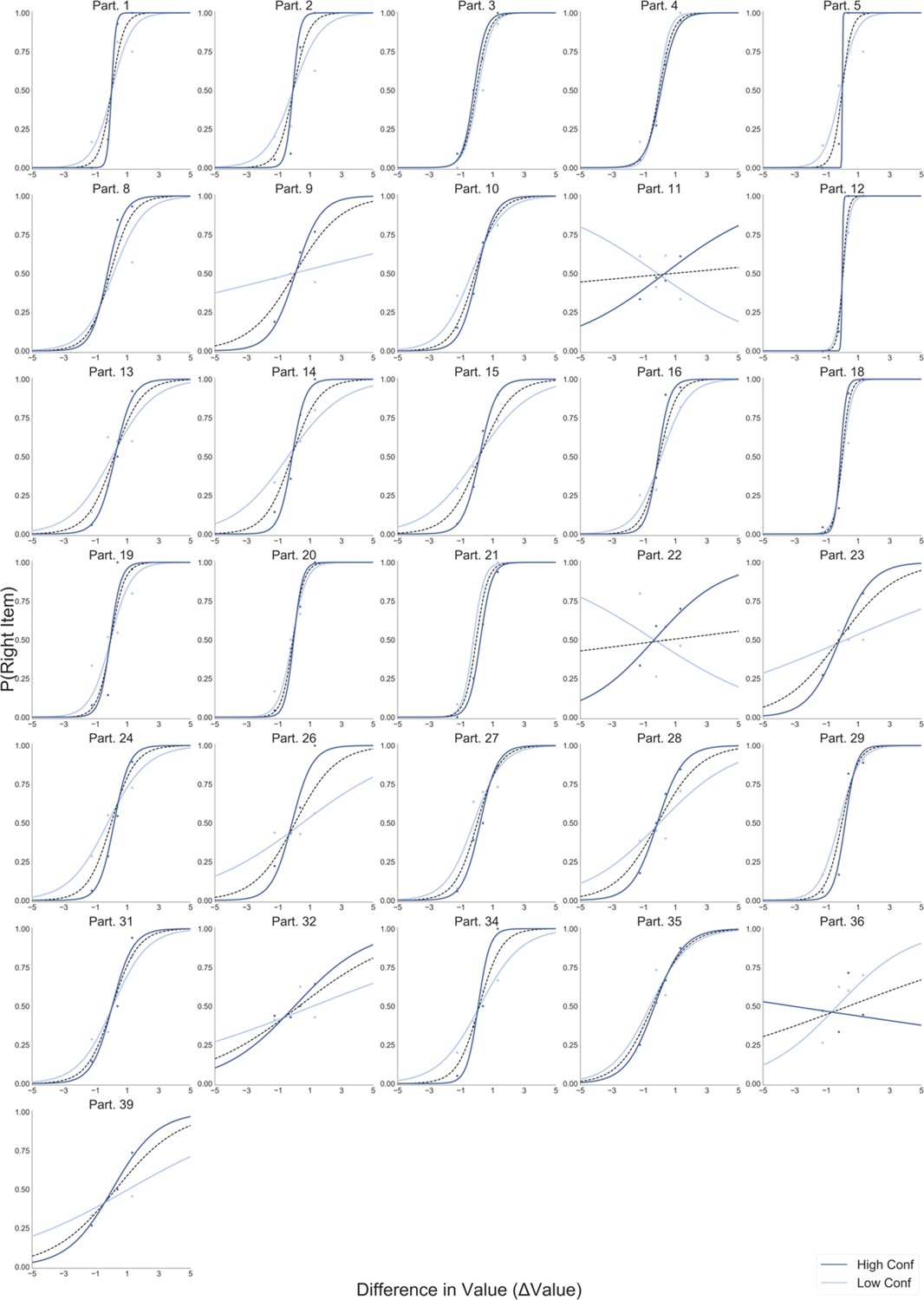
Logistic regression predicting choice from the difference in value between the two items (∆Value).
All participants in the Value Experiment, like frame, are presented. Light blue lines depict the logistic fit calculated using only low confidence trials. Dark blue lines show the logistic fit only for high confidence trials. Segmented black line considers the logistic regression calculated using all the trials.
Appendix 1—figure 3
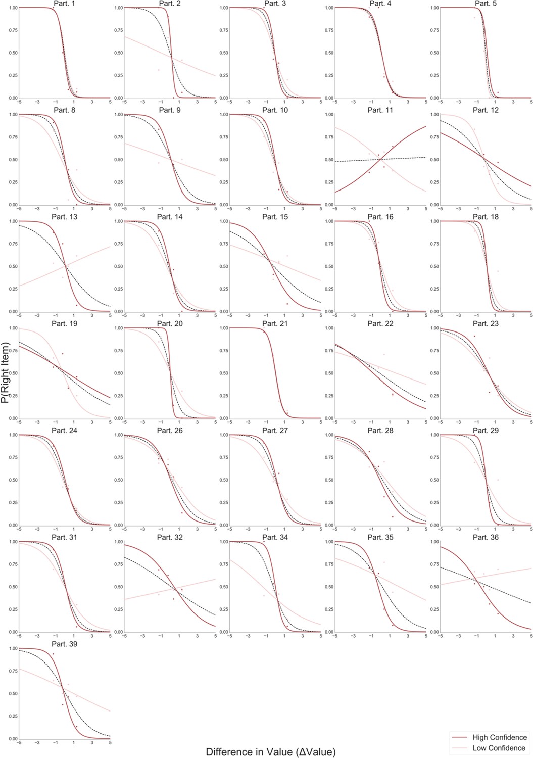
Logistic regression predicting choice from the difference in value between the two items (∆Value).
All participants in the Value Experiment, dislike frame, are presented. Light red lines depict the logistic fit calculated using low confidence trials. Dark red lines show the logistic fit using high confidence trials. Segmented black line considers the logistic regression calculated with all the trials.
Appendix 1—figure 4

Logistic regression predicting choice from the difference in number of dots between the two circles (∆Dots).
All participants in the Perceptual Experiment, most frame, are presented. Light blue lines depict the logistic fit calculated using only low confidence trials. Dark blue lines show the logistic fit only for high confidence trials. Segmented black line considers the logistic regression calculated with all the trials.
Appendix 1—figure 5
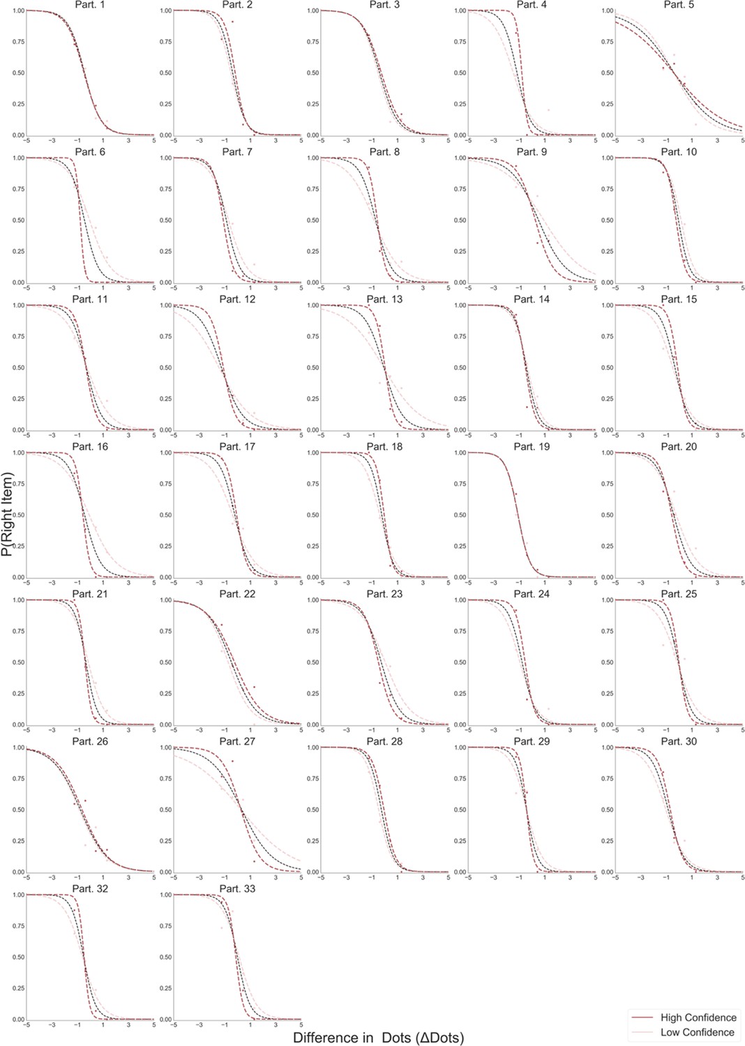
Logistic regression predicting choice from the difference in number of dots between the two circles (∆Dots).
All participants in the Perceptual Experiment, fewest frame, are presented. Light red lines depict the logistic fit calculated using only low confidence trials. Dark red lines show the logistic fit only for high confidence trials. Segmented black line considers the logistic regression calculated with all the trials.
Appendix 2—figure 1
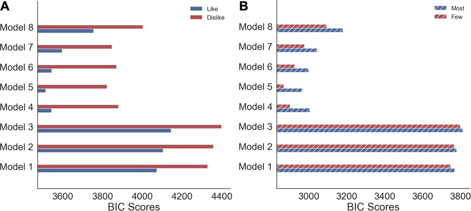
Model comparison of hierarchical logistic regressions for choice.
(A) Value and (B) Perceptual Experiments. Solid colour indicates the Value Experiment and striped colours indicate the Perceptual experiment.
Appendix 2—figure 2
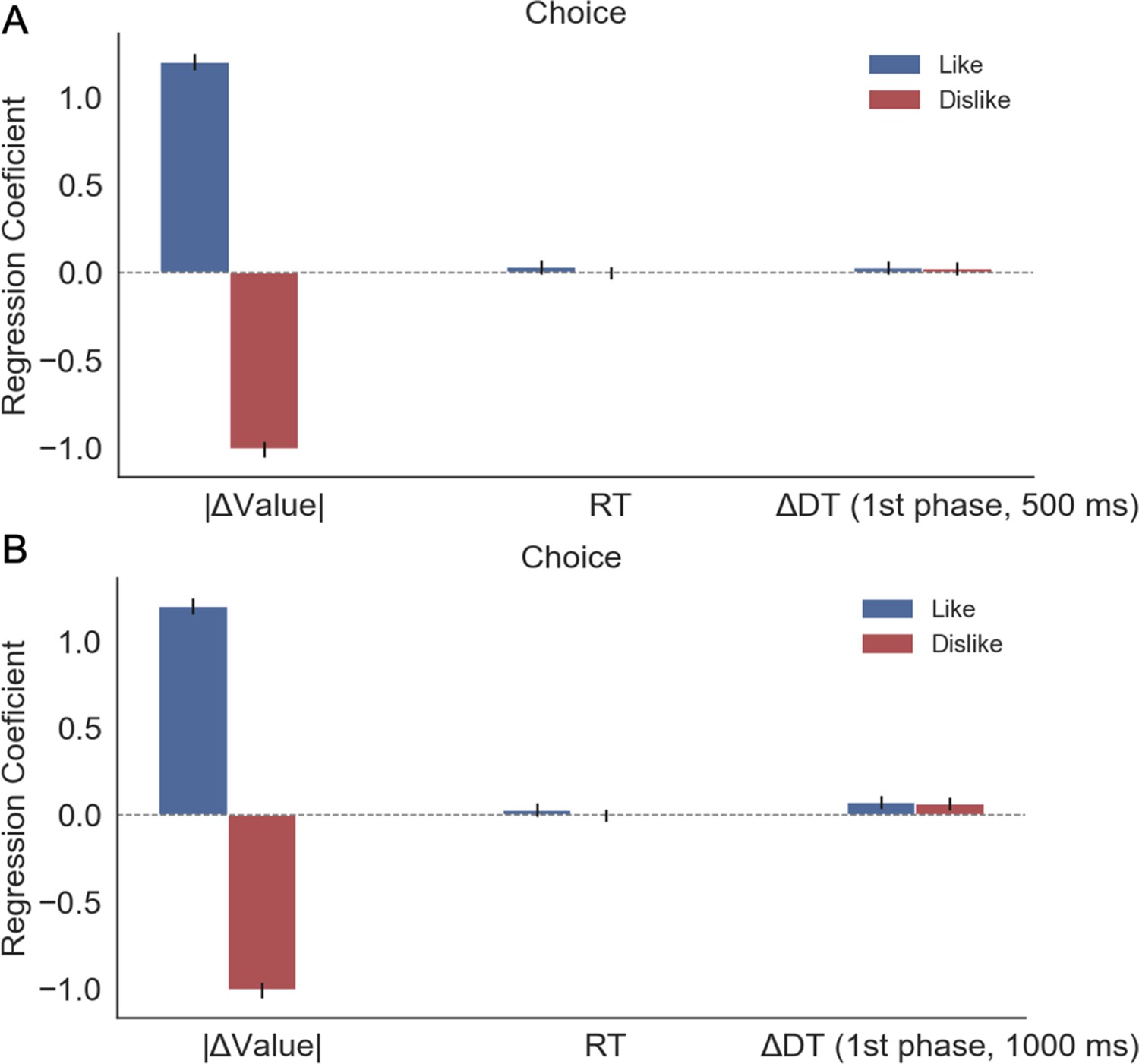
Kovach et al., 2014 conducted a study in which participants have to choose food items in ‘keep’ and ‘discard’ frames, in a similar way to our Value Experiment.
Gaze allocation was found to gravitate towards the chosen item overall, although during the initial moments of the trial (≈ 500 ms), they reported that gaze was directed towards the preferred item. To check if this effect appears in our Value Experiment we ran a regression model to predict choice (i.e. probability of choosing the item presented on the right side of the screen). We restricted the time to estimate ∆DT to the first 500 ms of the trial and used that variable as a predictor of choice in our model (A). We did not find a significant effect of gaze over choice in that period. This difference may be caused by the way the alternatives were presented during the decision time: while in Kovach et al., 2014 both alternatives were always displayed on screen during deliberation time, in our experiment the presentation was gaze contingent (i.e. participants needed to explore both items at the beginning of the trial to identify the available items). (B) We recalculated the model considering the initial 1000 ms of the trial and we observe how ∆DT starts to increase its effect over choice. The positive effect of ∆DT over choice is only significant (z = 1.97, p<0.05) in the like frame; in dislike frame the small effect is only a trend (z = 1.081, p=0.07). However, at 1000 ms ∆DT is already starting to be allocated to the option coherent with the behavioural responses required by the frame, not to preference.
Appendix 2—figure 3
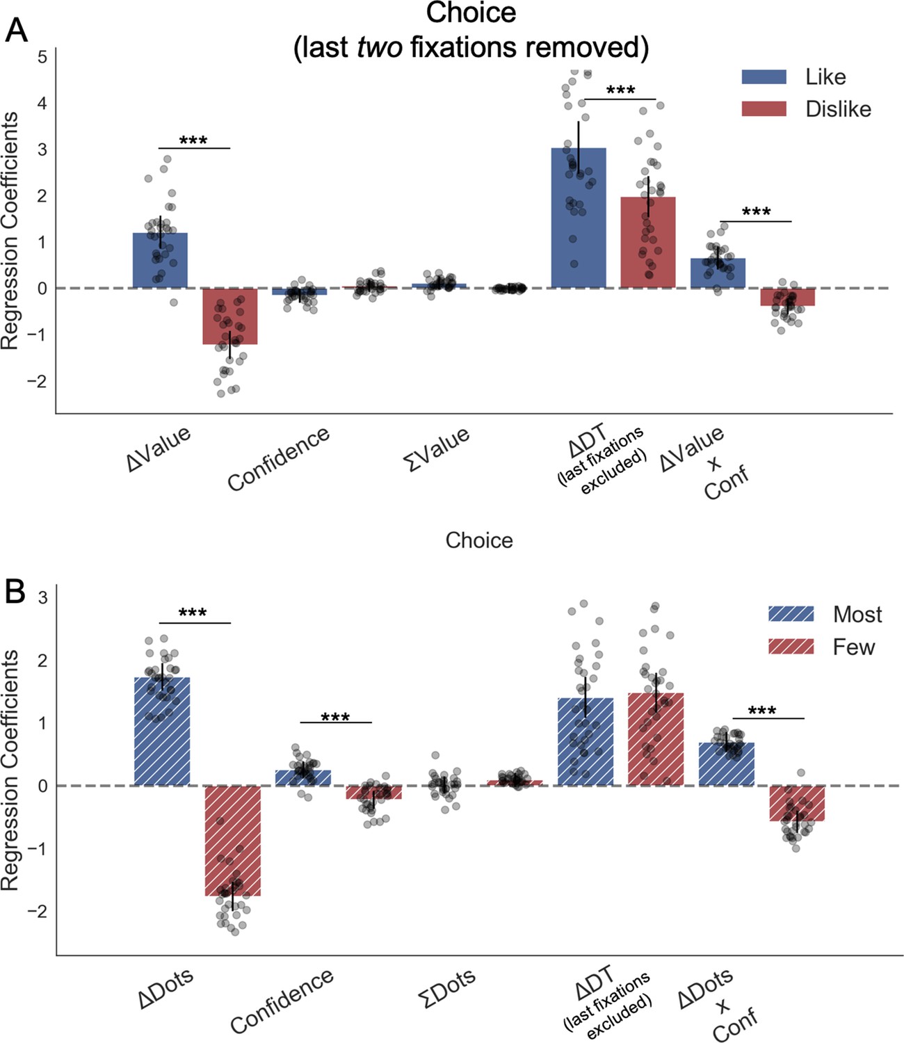
Choice behaviour excluding last fixations.
To assess the influence that last fixations have on the goal-relevant gaze asymmetries we repeated the hierarchical logistic modelling of choice (probability of choosing right item) in Value (B) and Perceptual (D) Experiments, excluding the last two fixations from the analysis. Note the two last fixations rather than only the last fixation, because this avoids statistical artifacts. All the results from the main analysis were confirmed: participants preferentially gazed at the item they chose in both frames (positive ∆DT effect in both experiments). All predictors were z-scored at the participant level. In both regression plots, bars depict the fixed-effects and dots the mixed-effects of the regression. Error bars show the 95% confidence interval for the fixed effect. In Value Experiment: ∆Value: difference in value between the two items (Valueright– Valueleft); RT: reaction time; ΣValue: summed value of both items; ∆DT: difference in dwell time (DTright– DTleft), excluding the last two fixations; Conf: confidence. In Perceptual Experiment: ∆Dots: difference in dots between the two circles (Dotsright– Dotsleft); ΣDots: summed number of dots between both circles. ***p<0.001, **p<0.01, *p<0.05.
Appendix 3—figure 1
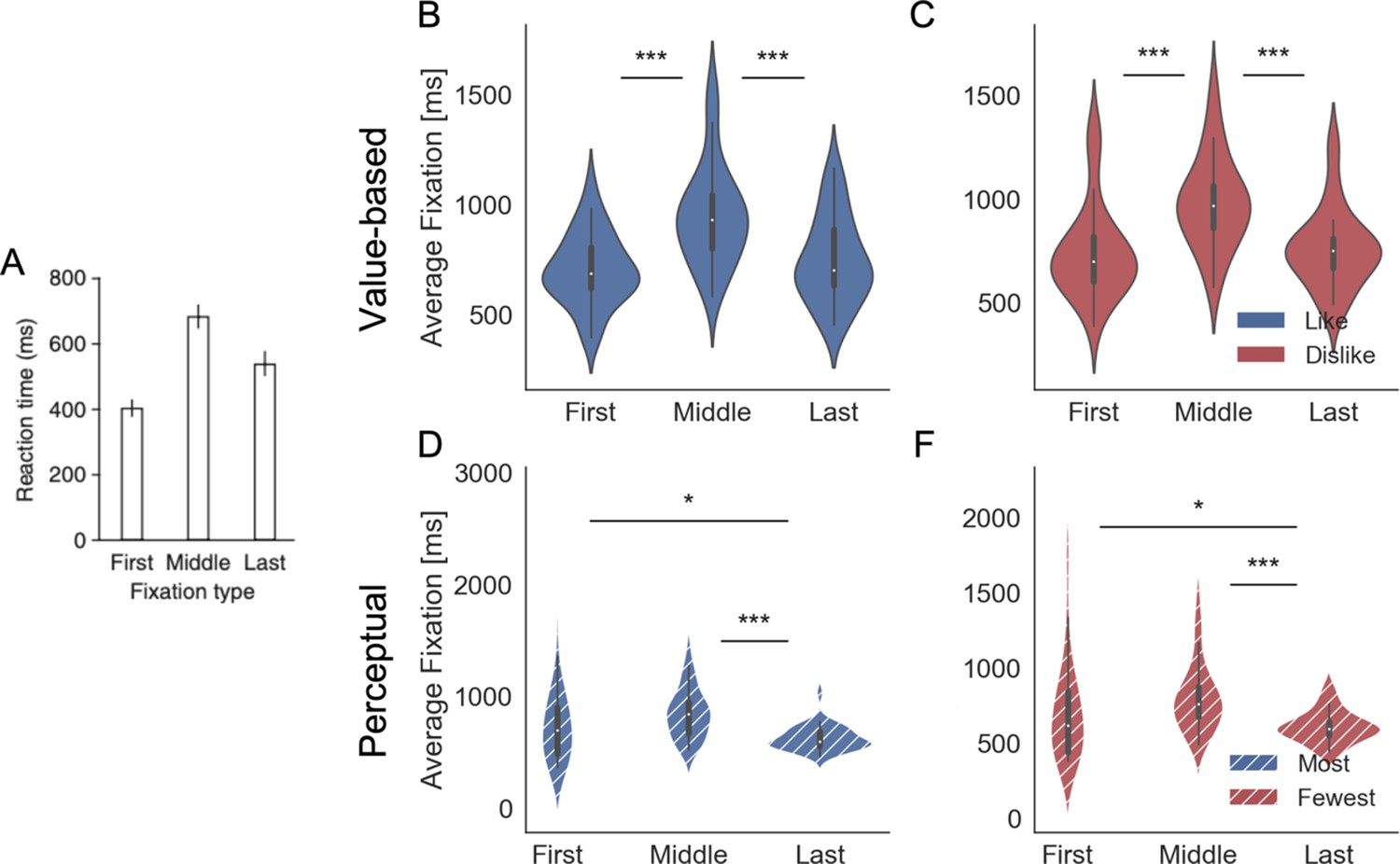
Fixation duration by type.
Middle fixations indicate any fixations that were not the first or last fixations of the trial. (A) In Krajbich et al., 2010 middle fixations were found to be longer than first and last fixations on average. For our Value Experiment, in like (B) and dislike (C) frames, and Perceptual Experiment, in most (D) and fewest (F) frames, the same pattern emerges with middle usually longer that first and last fixations. Violin plots depict the distribution of participant’s average fixation time. Panel A reproduced from Krajbich et al., 2010. ***p<0.001, **p<0.01, *p<0.05.
Appendix 3—figure 2
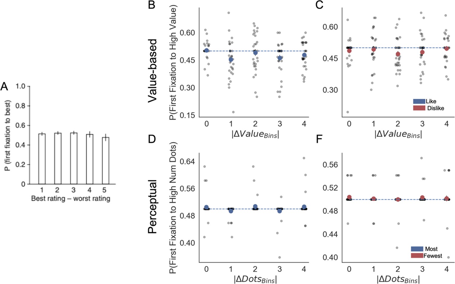
Fixation properties: probability that the first fixation is to the best item.
(A) Krajbich et al., 2010 reported that the probability is not significantly different from 50%, unaffected by the difference in ratings or difficulty (in our experiments difficulty is equivalent to the absolute difference item value, |ΔValue|, and absolute difference in number of dots, |ΔDots|). A similar pattern emerges in our Value Experiment, for like (B) and dislike (C) frames, and Perceptual Experiment, for most (D) and fewest (F) frames. Participant responses did not diverge from chance. Importantly, while in Krajbich et al., 2010 participants can see both alternatives from the beginning of the trial, our presentation was gaze contingent. Segmented blue line indicates chance level. Light grey dots correspond to individual participants’ probability of first fixation to high value/number of dots alternatives for each bin. Red or blue circles indicate the average for that bin considering all the participants. Panel A reproduced from Krajbich et al., 2010.
Appendix 3—figure 3
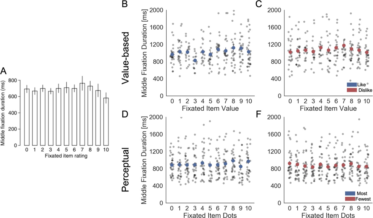
Fixation properties: middle fixation duration as a function of the rating (value or number of dots) of the fixated item.
(A) Krajbich et al., 2010 reported that middle fixations durations were independent of the value of the fixated items. In Value Experiment, we found that middle fixation duration was independent of the value of the fixated item in like frame (B); however, a slight yet significant effect in dislike (C) frame was found (hierarchical linear regression estimate: βDislike = 0.025, t(27.35) = 3.441, p<0.001). In the Perceptual Experiment, for the most (D) frame we found a significant effect of fixated value (βMost = 0.017, t(29.51) = 3.013, p<0.01), but not for fewest (F) frame. Light grey dots correspond to individual participants’ middle fixation durations for each bin. Red or blue circles indicate the average for that bin considering all the participants. For the hierarchical linear regression, z-scored data at participant levels was used. Panel A reproduced from Krajbich et al., 2010.
Appendix 3—figure 4
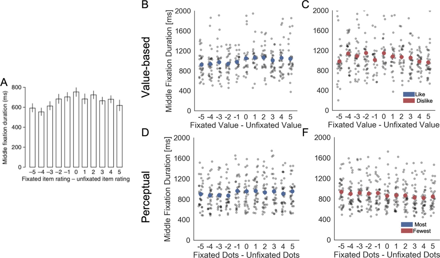
Fixation properties: middle fixation duration as a function of the difference in ratings (value or number of dots) between the fixated and unfixated items.
(A) Krajbich et al., 2010 reported a slight but significant dependency of middle fixations durations on the difference in value between items. In our Value Experiment, we found that in like (B) and dislike (C) this relationship was significant (hierarchical linear regression estimate: βLike = 0.015, t(28.22) = 2.192, p<0.05; βDislike = -0.027, t(28.22) = -4.415, p<0.001). Similarly, in the Perceptual Experiment, most (D) and fewest (F) frames, the dependence was found also significant (βMost = 0.01, t(29.51) = 2.663, p<0.01; βFew = -0.027, t(29.51) = -6.330, p<0.001). Interestingly, a positive sign of the effect in like and most frames indicates that middle fixations tend to be longer for the option with the higher value or number of dots. On the other hand, the negative sign of the effect indicates that middle fixations would be longer for the option with lower value or number of dots in dislike and fewest frames. Light grey dots correspond to individual participants’ middle fixation durations for each bin. Full red or blue circles indicate participant’s average. Data are binned across participants for visualisation. All the factors and the predicted variable in the hierchical regression were z-scored at participant level. Panel A reproduced from Krajbich et al., 2010.
Appendix 3—figure 5
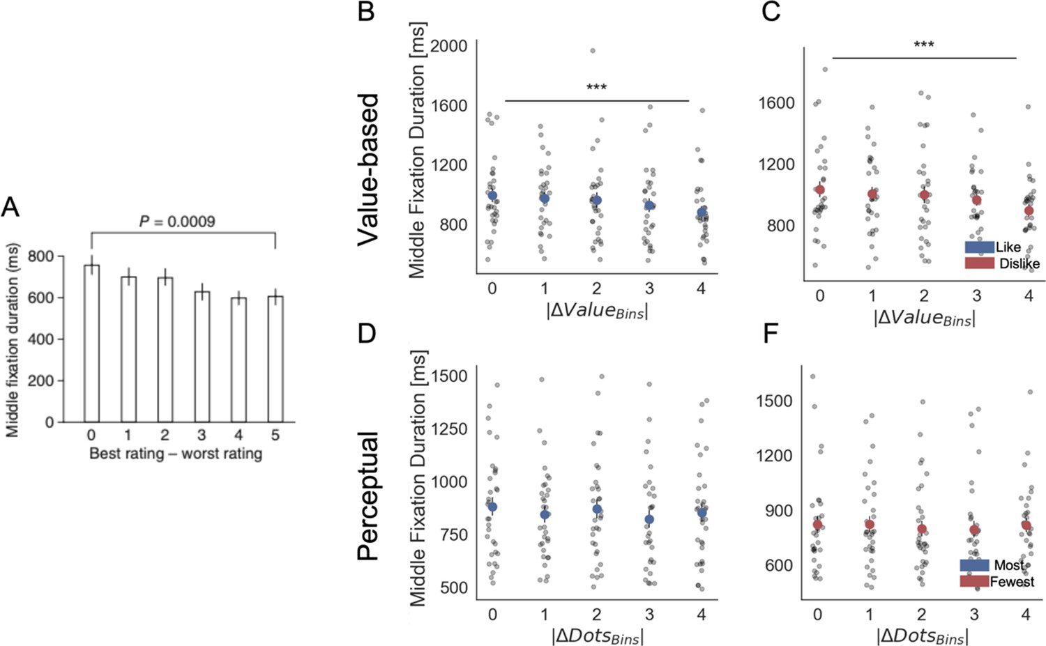
Fixation properties: middle fixation duration as a function of the difference in ratings between the best- and worst-rated items (difficulty of the trial).
In our experiments, |ΔValue| and |ΔDots| represent the difficulty of the trials. (A) Krajbich et al., 2010 reported a dependency of middle fixations durations on difficulty, with longer fixations in more difficult decisions. In our Value Experiment, in like (B) and dislike (C) frames a similar pattern was found: longer middle fixations for more difficult (lower |ΔValue|) trials (hierarchical linear regression estimate: βLike = -0.029, t(28.22) = -2.262, p<0.05; βDislike = -0.047, t(28.22) = -4.415, p<0.001). The same relationship was found only in the most frame (D) but no in the fewest frame (F) in the Perceptual Experiment (βMost = -0.037, t(29.51) = -3.985, p<0.001; βFew = -0.024, t(29.51) = -1.623, p=0.10). Light grey dots correspond to individual participants’ middle fixation durations for each bin. Full red or blue circles indicate participant’s average. Data are binned across participants for visualisation. All the factors and the predicted variable in the hierchical regression were z-scored at participant level. Panel A reproduced from Krajbich et al., 2010. Tests presented here are based on a paired two-sided t-test between the first and last bin.***p<0.001, **p<0.01, *p<0.05.
Appendix 4—figure 1

Model comparison of hierarchical linear regressions for confidence.
(A) Value and (B) Perceptual Experiments. Solid colour indicates the value-based experiment and striped colours indicate the perceptual experiment.
Appendix 5—figure 1
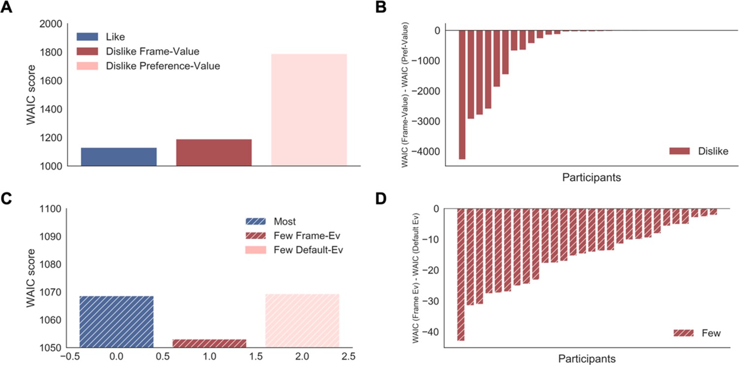
GLAM model comparison.
(A) Average WAIC scores for like and dislike GLAM models fitted at individual level. In the dislike frame, two possible models are compared: preference-value, value reported in the BDM bid was used directly to fit the data; and frame-value, value was adjusted to comply with the frame modification (see Methods for more details). The model accounting for goal-relevant evidence in the dislike frame had a better fit. (B) Individual WAIC differences between dislike models fitted with frame-value and preference-value. Negative differences indicate best fits for the frame-value in all the participants. (C) Average WAIC scores for most and fewest GLAM models fitted at individual level. In the fewest frame, two possible models are compared: default-evidence, the number of dots was used directly to fit the data, and frame-evidence, evidence was adjusted to comply with the frame modification (i.e. the opposite of the number of dots was used as evidence). (D) Individual WAIC differences between fewest models fitted with frame-evidence and default-evidence. Negative differences indicate best fits for the frame-evidence in all the participants. Solid colour indicates the value-based experiment and striped colours indicate the perceptual experiment.
Appendix 5—figure 2
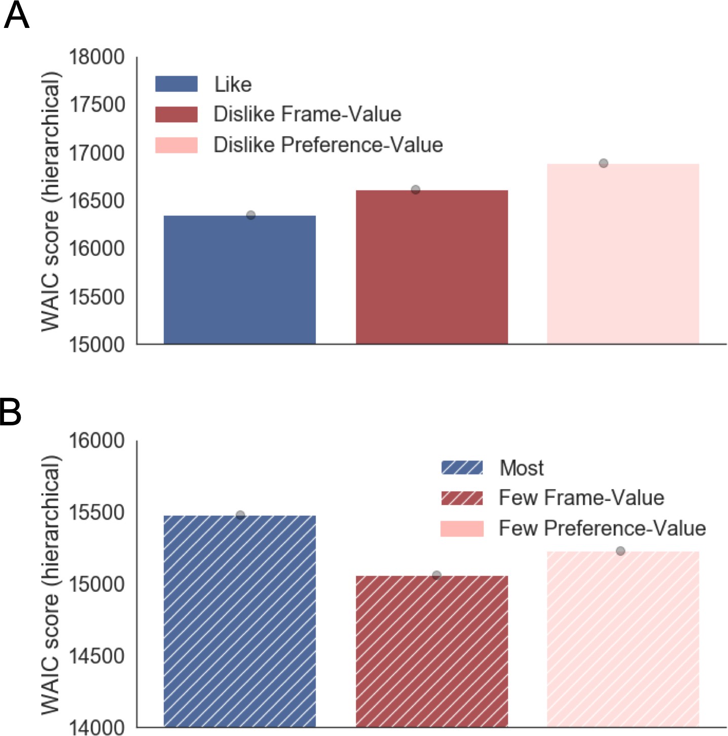
Hierarchical GLAM model comparison.
(A) Value Experiment. WAIC scores for like and dislike GLAM models fitted hierarchically. In the dislike frame, two possible models are compared: preference-value, input values corresponding to the preferences reported at the beginning of the experiment (BDM bid); and frame-value, in which value was adjusted to comply with the frame modification (see Methods for more details). In dislike frame, the model accounting for goal-relevant resulted the most parsimonious of the two. (B) Perceptual Experiment. WAIC scores for most and fewest GLAM models fitted hierarchically. In the fewest frame, two possible models are compared: default-evidence, the number of dots was used directly to fit the data, and frame-evidence, evidence was adjusted to comply with the frame modification (i.e. the opposite of the number of dots was used as evidence).
Appendix 5—figure 3
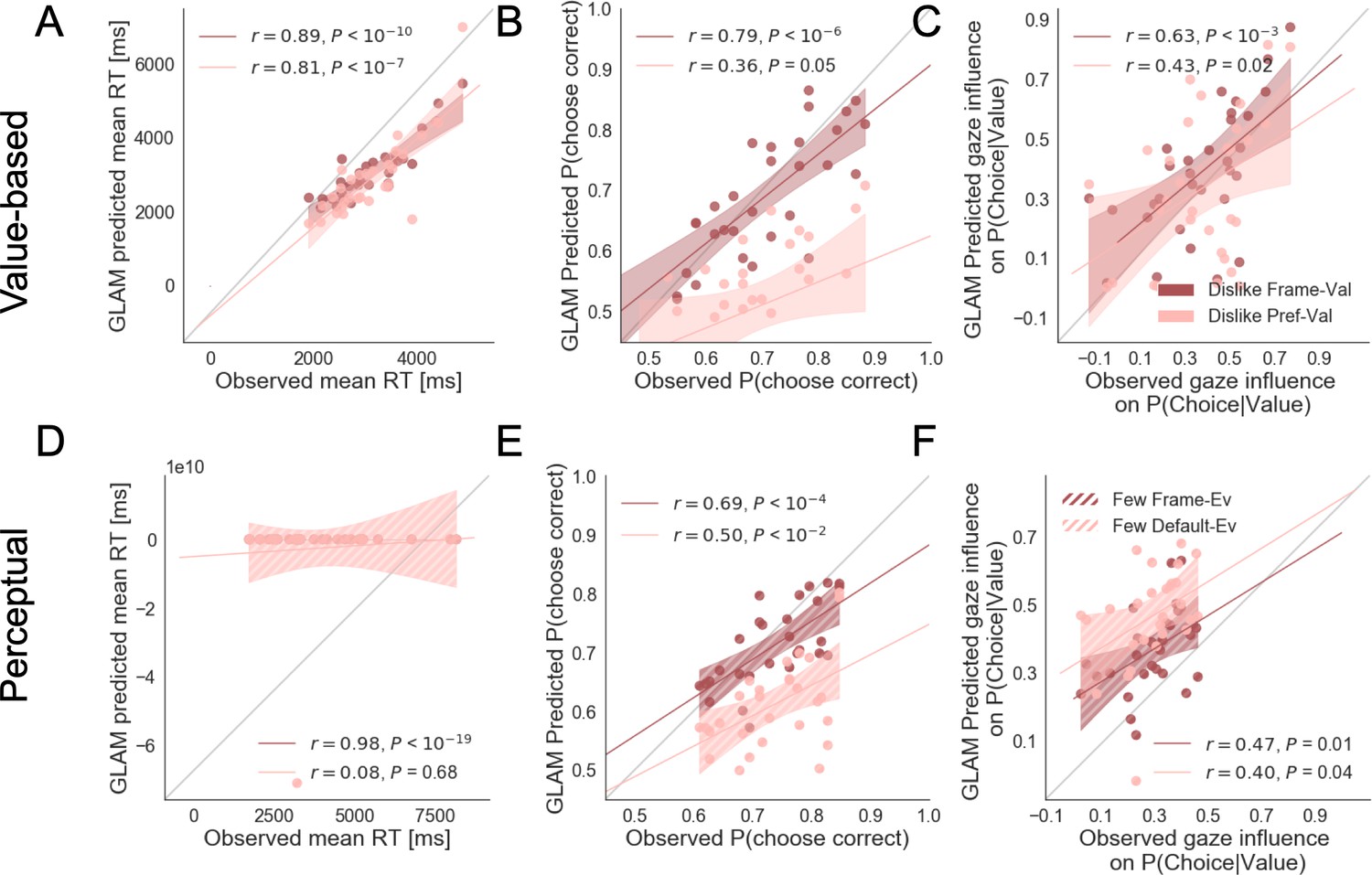
Individual out-of-sample prediction from the GLAM model for behavioural measures in Value (dislike) (A–C) and Perceptual (fewest) Experiments (D–F).
In the dislike frame, two models are used to generate simulations: preference-value, value reported in the BDM bid was used directly to fit GLAM model; and frame-value, the values were adjusted to comply with the frame modification. The model predicts participants mean reaction time (RT) (A), probability of choosing the best item (i.e. item with lower value) (B) and the influence of gaze in choice probability (C, check Results section for more details on gaze influence measure). The frame-value model correlates better with the observed data. In the Perceptual Experiment, fewest frame, also two possible models are used to generate simulations: default-evidence, the number of dots was used directly to fit the data, and frame-evidence, the evidence was adjusted to comply with the context modification (i.e. opposite of the number of dots). We show the correlation between the data and simulations for RT (D), the probability of choosing the best alternative (i.e. alternative with fewer dots) (E) and gaze influence (F). In this case, frame-evidence model also predicts the behaviour in the fewest frame better. The results corresponding to the models using frame-evidence are presented in red and the models using default-evidence in pink. Dots depict the average of predicted and observed measures for each participant. Lines depict the slope of the correlation between observations and the predictions. The shadowed region presents the 95% confidence intervals, with full colour representing Value Experiment and striped colour the Perceptual Experiment. Model predictions are simulated using parameters estimated from individual fits for even-numbered trials.
Appendix 5—figure 4

Replication of behavioural effect of interest by simulations using the GLAM fitted for like (A) and most frames (B).
The four panels present four relevant behavioural relationships found in the data: (top left) faster responses (shorter RT) when the choice is easier (i.e. easier choices are found with higher |ΔValue| in value-based and higher |ΔDots| in perceptual); (top right) probability of choosing the right alternative increases when the difference in evidence (value or number of dots) is higher in the alternative at the right side of the screen (ΔValue and ΔDots are calculated considering right minus left options); (bottom left) the probability of choosing an alternative depends on the gaze difference; and (bottom right) the gaze influence on choice depending on the difference in gaze time between both alternatives. Solid blue dots depict the mean of the data across participants in like and most frames. Light blue dots present the mean value for each participant. In the Value Experiment, the solid grey lines show the average for model simulations. In the Perceptual Experiment, segmented grey lines show the model simulations. Data are binned for visualisation.
Appendix 5—figure 5
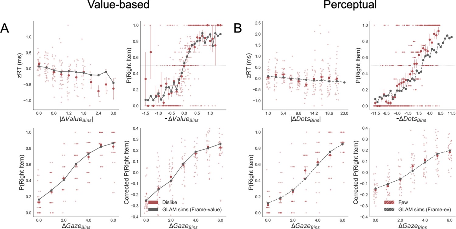
Replication of behavioural effect of interest by simulations using the GLAM fitted for dislike (A) and fewest frames (B).
Frame-relevant evidence was used to fit the model. The four panels present four relevant behavioural relationships found in the data. Top left: faster responses (shorter RT) when the choice is easier (i.e. easier choices are found with higher |ΔValue| in value-based and higher |ΔDots| in perceptual). Top right: probability of choosing the right alternative increases when the difference in evidence (value or number of dots) is lower in the alternative at the right side of the screen (notice that -ΔValue and -ΔDots are calculated considering left minus right options). Bottom left: the probability of choosing the right alternative depends on the gaze difference favouring the right option. Bottom right: the gaze influence on choice depending on the difference in gaze time between both alternatives. Solid red dots depict the mean of the data across participants in dislike and fewest frames. Light red dots present the mean value for each participant. In the Value Experiment, the solid grey lines show the average for model simulations. In the Perceptual Experiment, segmented grey lines show the model simulations. Data are binned for visualisation.
Appendix 5—figure 6
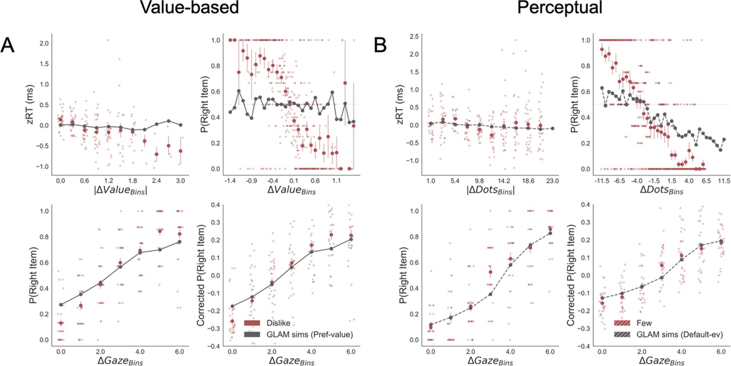
Replication of behavioural effect of interest by simulations using the GLAM fitted for dislike (A) and fewest frames (B).
In this case, the models were fitted without adapting the values and dot numbers to the evidence that was relevant for the particular frame, that is the preference value and the default number of dots were used to fit the model in the dislike and fewest frame, respectively. The four panels present four relevant behavioural relationships found in the data. Top left: faster responses (shorter RT) when the choice is easier (i.e. easier choices are found with higher |ΔValue| in value-based and higher |ΔDots| in perceptual). Top right: probability of choosing the right alternative increases when the difference in evidence (value or number of dots) is lower in the alternative at the right side of the screen (ΔValue and ΔDots are calculated consider right minus left options). Bottom left: the probability of choosing the right alternative depends on the gaze difference favouring the right option. Bottom right: the gaze influence on choice depending on the difference in gaze time between both alternatives. No replication of the behavioural effect was found in this case for the relationship between RT -|ΔValue| and RT -|ΔDots| in dislike and fewest frames, respectively. Also P(right item)-ΔValue and P(right item)-ΔDots relationship was not replicated in dislike and fewest frames, respectively. Gaze effect seem to still keep its relationship, since gaze allocation time was not modified to account for the frame shift. Solid red dots depict the mean of the data across participants in dislike and fewest frames. Light red dots present the mean value for each participant. In the Value Experiment, the solid grey lines show the average for model simulations. In the Perceptual Experiment, segmented grey lines show the model simulations. Data are binned for visualisation.
Appendix 6—figure 1
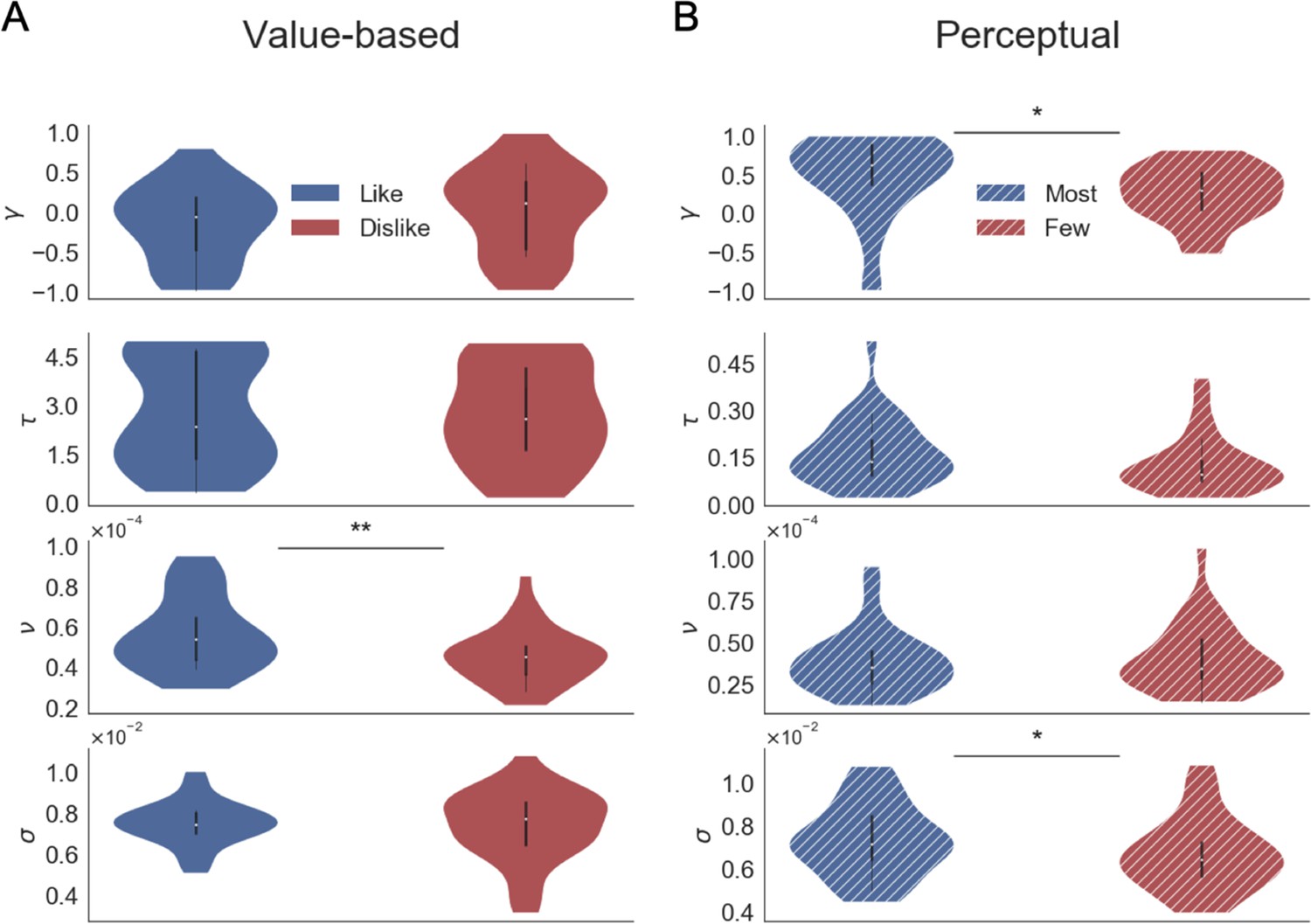
Parameters fitted at subject level using GLAM in Value (A) and Perceptual (B) Experiments.
The free parameters are γ (gaze bias), τ (evidence scaling), ν (drift term), and σ (standard deviation of the normally distributed noise). In the Value Experiment, we found a significant decrease in the drift term during the dislike frame, maybe indicating a more uncertain decision process. The parameters in Perceptual Experiment were significantly different for gaze bias and noise term, with higher γ and σ values in the most frame. This may indicate a reduced effect of gaze on choice during the most frame and slightly less noisier accumulation process in the fewest frame. In each experiment, the GLAM parameters were fitted independently for each frame. In the violin plot, red and blue areas indicate the distribution of the parameters across participants. Black bars present the 25, 50, and 75 percentiles of the data. Solid colour indicates the Value Experiment and striped colours indicate the Perceptual Experiment.
Appendix 6—figure 2
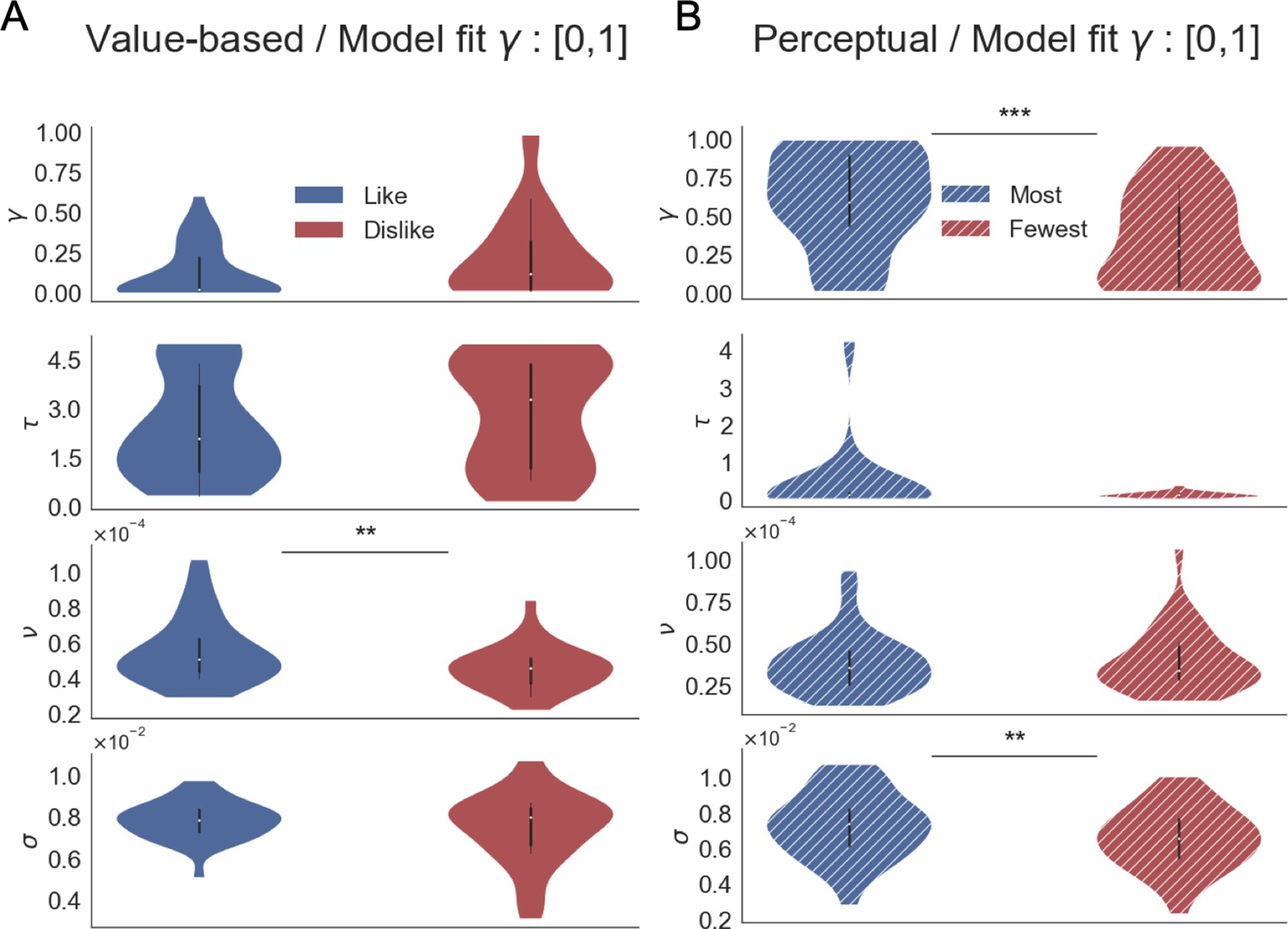
GLAM model parameters when the model fit is performed constraining γ to [0,1] range.
Thomas et al., 2019 describes a ‘leakage’ of evidence when γ < 0, which can be a conflicting assumption in this type of models. We corroborated that the differences between the parameters in like/dislike and most/fewest remain the same in comparison to the fit reported constraining γ to [−1,1].
Appendix 7—figure 1
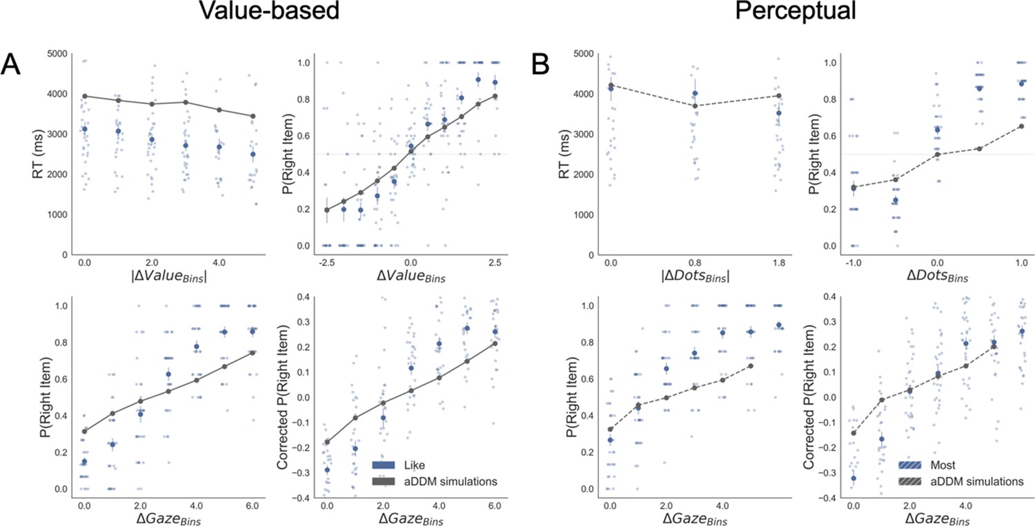
Replication of behavioural effects by aDDM simulations for like (A) and most frames (B).
The four panels present four relevant behavioural relationships found in the data. Top left: faster responses (shorter reaction time, RT) when the choice is easier (i.e. easier choices are found with higher |ΔValue| and |ΔDots| in Value an Perceptual Experiments, respectively). Top right: probability of choosing the right alternative increases when the evidence towards the right item is higher (ΔValue and ΔDots are calculated considering right minus left options). Bottom left: the probability of choosing the item on the right side of the screen depends on the gaze time difference (ΔGaze, calculated as the time observing the right minus the left item). Bottom right: gaze influence on choice depending on the difference in ΔGaze (check Results section for more details on gaze influence). Solid blue dots depict the mean of the data across participants in like and most frames. Light blue dots show the mean value for each participant. In Value Experiment, the solid grey lines show the average for model simulations. In the Perceptual Experiment, segmented grey lines show the average for model simulations. Data and simulations were binned for visualisation.
Appendix 7—figure 2
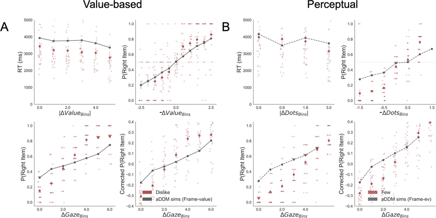
Replication of behavioural effects by aDDM simulations for dislike (A) and fewest (B) frames.
Importantly, these models were fitted using goal-relevant evidence. The four panels present four relevant behavioural relationships found in the data. Top left: faster responses (shorter reaction time, RT) when the choice is easier (i.e. easier choices are found with higher |ΔValue| and |ΔDots| in Value and Perceptual Experiments, respectively). Top right: probability of choosing the right alternative increases when the evidence towards the left item is higher (-ΔValue and –ΔDots, that is, increment when left item is more valuable or has more dots than the right item). Bottom left: the probability of choosing the item on the right side of the screen depends on the gaze time difference (ΔGaze, calculated as the time observing the right minus the left item). Bottom right: gaze influence on choice depending on the difference in ΔGaze (check Results section for more details on gaze influence). Solid red dots depict the mean of the data across participants in dislike and fewest frames. Light red dots show the mean value for each participant. In Value Experiment, the solid grey lines show the average for model simulations. In the Perceptual Experiment, segmented grey lines show the average for model simulations. Data and simulations were binned for visualisation.
Appendix 7—figure 3
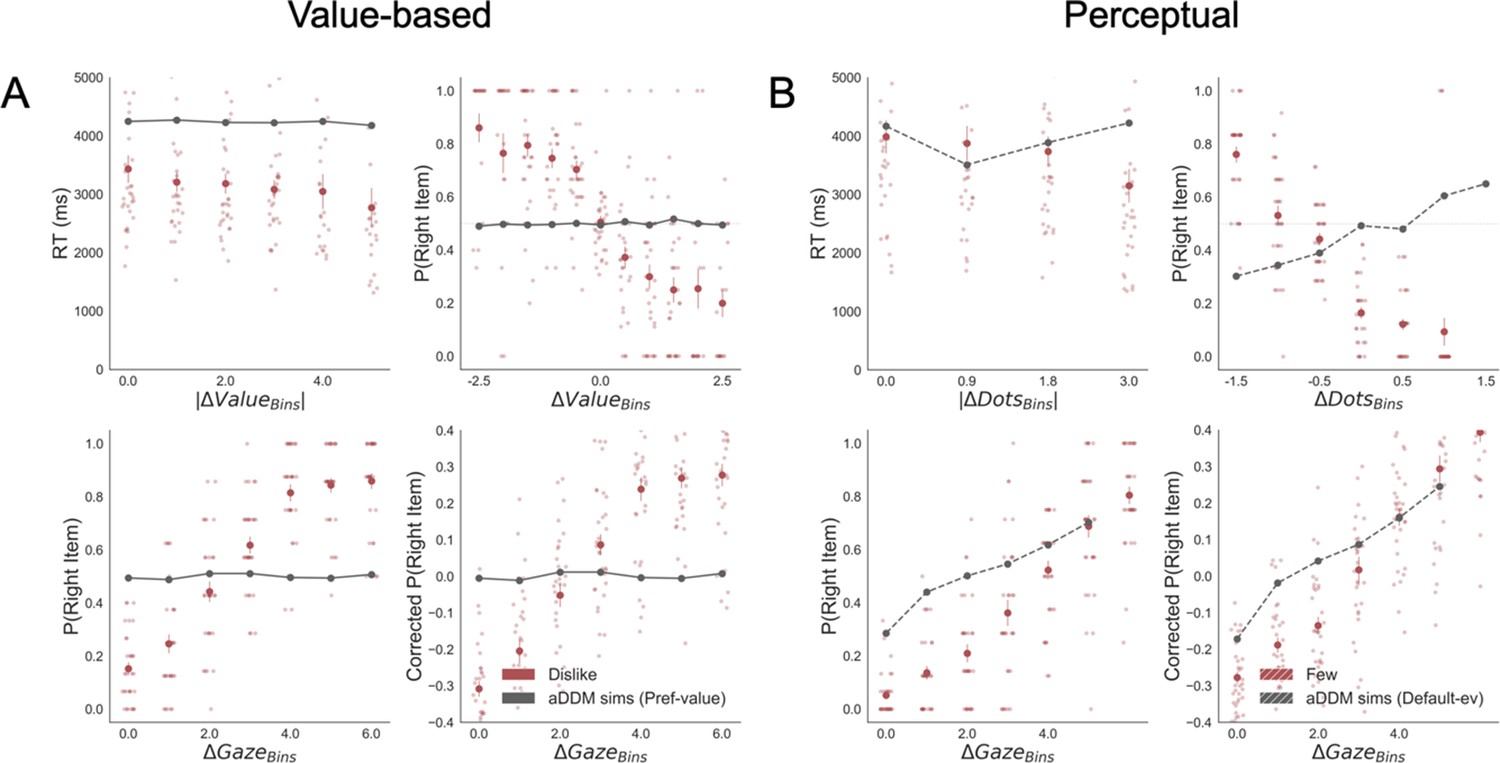
Replication of behavioural effects by aDDM simulations for dislike (A) and fewest frames (B).
Importantly, these models were fitted using the default evidence in Value and Perceptual Experiments, that is, preference value and number of dots, respectively. Unlike the models fitted with goal-relevant evidence, these models do not capture reaction time (RT) and choice behaviour in dislike and fewest frames. The four panels present four relevant behavioural relationships found in the data. Top left: faster responses (shorter RT) when the choice is easier (i.e. easier choices are found with higher |ΔValue| and |ΔDots| in Value an Perceptual Experiments, respectively). Top right: probability of choosing the right alternative increases when the evidence towards the left item is higher (ΔValue and ΔDots are calculated considering right minus left options). Bottom left: the probability of choosing the item on the right side of the screen depends on the gaze time difference (ΔGaze, calculated as the time observing the right minus the left item). Bottom right: gaze influence on choice depending on the difference in ΔGaze (check Results section for more details on gaze influence). Solid red dots depict the mean of the data across participants in dislike and fewest frames. Light blue dots show the mean value for each participant. In Value Experiment, the solid grey lines show the average for model simulations. In the Perceptual Experiment, segmented grey lines show the average for model simulations. Data and simulations were binned for visualisation.
Appendix 8—figure 1
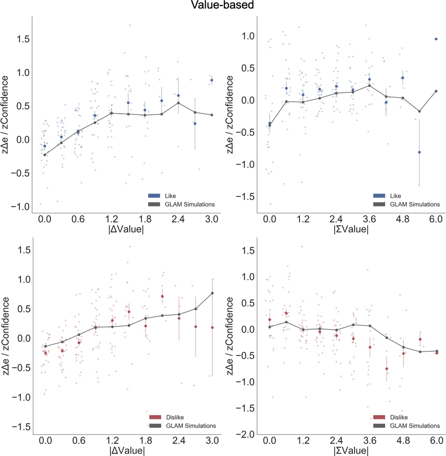
Balance of evidence simulations in the Value Experiment.
The difference between accumulators (Δe) obtained from GLAM simulations matches participants’ confidence. Top left: a higher value difference between the two items (|ΔValue|) increases confidence and simulated Δe. Top right: in the like frame, an increase in the summed value of the two alternatives (|ΣValue|) boosts confidence and simulated Δe. Bottom left: as in like frame, |ΔValue| boosted confidence and Δe in dislike frame. Bottom right: in the dislike frame, the effect of |ΣValue| over confidence flips: confidence and Δe decrease with higher values of the alternatives, accounting for the change in goal. Blue and red dots depict the (z-scored) confidence taken from participants in like and dislike frames (respectively). Grey line presents the model simulations for both separate frames. Data were segmented in 11 bins for ΔValue or ΣValue.
Appendix 8—figure 2
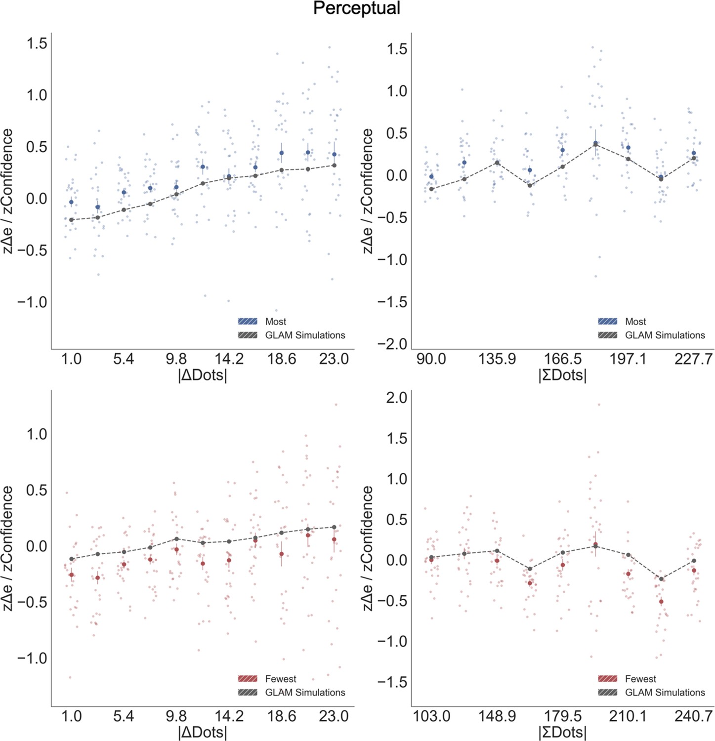
Balance of evidence simulations in the Perceptual Experiment.
As in Value Experiment, the difference between accumulators (Δe) obtained from GLAM simulations matches participants’ confidence. Top left: a higher difference in number of dots between the two circles (|ΔDots|) increases confidence and simulated Δe. Top right: in the most frame, an increase in the summed number of dots (|ΣDots|) boosts confidence and simulated Δe. Bottom left: as in most frame, |ΔDots| boosted confidence and Δe in fewest frame. Bottom right: in the fewest frame, the effect of |ΣDots| over confidence flips: confidence and Δe decrease with higher number of dots in both circles, accounting for the change in goal. Blue and red dots depict the (z-scored) confidence taken from participants in most and fewest frames (respectively). Grey line presents the model simulations for both separate frames. Data were segmented in 11 bins for ΔDots or ΣDots.
Appendix 8—figure 3
Pooled linear regressions to predict balance of evidence (Δe) simulations.
Here the full model results for Figure 6 (see Results section) are displayed. In Value Experiment, the full simulations of Δe replicated the pattern of results obtained in human data (confidence results), that is there is a flip in the sign of ΣValue effect over confidence between like (A) and dislike (D) frames. However, if the gaze asymmetry is removed, we found the effect of ΣValue over Δe disappears. The results in Perceptual Experiment, most (B) and fewest (E) frames, mirror the findings in the Value Experiment.
Tables
Appendix 2—table 1
Hierarchical logistic models for choice.
| Models | Formulas |
|---|---|
| Model 1 | Choice ~ ∆Value |
| Model 2 | Choice ~ ∆Value + Confidence |
| Model 3 | Choice ~ ∆Value + Confidence + ΣValue |
| Model 4 | Choice ~ ∆Value + Confidence + ΣValue + ∆DT |
| Model 5 | Choice ~ ∆Value + Confidence + ΣValue + ∆DT + ∆Value * Confidence |
| Model 6 | Choice ~ ∆Value + Confidence + ΣValue + ∆DT + ∆Value * Confidence + ∆Value * ΣValue |
| Model 7 | Choice ~ ∆Value + Confidence + ΣValue + ∆DT + ∆Value * Confidence + ∆Value * ΣValue + Confidence * ∆DT |
| Model 8 | Choice ~ ∆Value + Confidence + ΣValue + ∆DT + GSF + ∆Value * Confidence + ∆Value * ΣValue + Confidence * ∆DT + ∆Value * GSF |
Appendix 2—table 2
Statistical results for the hierarchical linear models for choice in Value Experiment.
Z-values for the regression coefficients and their statistical significance are presented for both frames. To check significant differences of the regression coefficients between like and dislike frames repeated samples t-tests between the participants’ regression coefficients were calculated.
| Choice value experiment (n = 31) | ||||||
|---|---|---|---|---|---|---|
| Like | Dislike | Like - Dislike | ||||
| Z | P | Z | P | T | P | |
| ∆Value | 7.917 | <0.001 | −8.652 | <0.001 | 10.74 | <0.001 |
| ∆DT | 6.448 | <0.001 | 6.75 | <0.001 | 2.31 | <0.05 |
| ∆Value x Conf | 5.446 | <0.001 | −4.681 | <0.001 | 9.55 | <0.001 |
-
*Confidence and ΣValue did not have a significant effect over choice in the regression.
Appendix 2—table 3
Statistical results for the hierarchical logistic models for choice in Perceptual Experiment.
Z-values for the regression coefficients and their statistical significance are presented for both frames. Repeated samples t-tests between the participants’ regression coefficients in most and fewest frames were calculated.
| Choice perceptual experiment (n = 32) | ||||||
|---|---|---|---|---|---|---|
| Most | Fewest | Most - Fewest | ||||
| Z | P | Z | P | T | P | |
| ∆Dots | 14.905 | <0.001 | −14.394 | <0.001 | 30.32 | <0.001 |
| Confidence | −2.823 | <0.01 | −6.705 | <0.001 | 6.67 | <0.001 |
| ∆DT | 10.249 | <0.001 | 10.449 | <0.001 | −2.17 | <0.05 |
| ∆Dots x Conf | 8.677 | <0.001 | −6.23 | <0.001 | 23.69 | <0.001 |
-
*ΣDots did not have a significant effect over choice in the regression.
Appendix 4—table 1
Hierarchical linear models for confidence.
| Models | Formulas |
|---|---|
| Model 1 | Confidence ~ |∆Value| |
| Model 2 | Confidence ~ |∆Value| + RT |
| Model 3 | Confidence ~ |∆Value| + RT + GSF |
| Model 4 | Confidence ~ |∆Value| + RT + GSF + ΣValue |
| Model 5 | Confidence ~ |∆Value| + RT + GSF + ΣValue + ∆DT |
Appendix 4—table 2
Statistical results for the hierarchical linear models for confidence in Value Experiment.
Z-values for the regression coefficients and their statistical significance are presented for the two frames. Repeated samples t-tests between the participants’ regression coefficients in like and dislike frames were calculated.
| Confidence value experiment | ||||||
|---|---|---|---|---|---|---|
| Like | Dislike | Like - Dislike | ||||
| Z | P | Z | P | T | P | |
| |∆Value| | 5.465 | <0.001 | 6.3 | <0.001 | −4.72 | <0.01 |
| RT | −6.373 | <0.001 | −7.739 | <0.001 | ns | |
| GSF | −2.365 | <0.05 | −2.589 | <0.05 | ns | |
| ΣValue | 3.206 | <0.001 | −4.492 | <0.001 | 9.91 | <0.001 |
Appendix 4—table 3
Statistical results for the hierarchical linear models for confidence in Perceptual Experiment.
Z-values for the regression coefficients and their statistical significance are presented for the two frames. Repeated samples t-tests between the participants’ regression coefficients in most and fewest frames were calculated.
| Confidence perceptual experiment | ||||||
|---|---|---|---|---|---|---|
| Most | Fewest | Most - Fewest | ||||
| Z | P | Z | P | T | P | |
| |∆Value| | 3.546 | <0.001 | 7.571 | <0.001 | −4.554 | <0.001 |
| RT | −7.599 | <0.001 | −5.51 | <0.001 | ns | |
| GSF | −4.354 | <0.001 | −5.204 | <0.001 | ns | |
| ΣDots | 2.061 | <0.05 | −7.135 | <0.001 | 14.621 | <0.001 |
Appendix 7—table 1
aDDM model parameters.
Estimated parameters for Value and Perceptual Experiments. Parameter description - d: speed of integration; σ: standard deviation for the noise distribution, θ: attentional bias. NNL: negative log-likelihood of the models indicating goodness-of-fit.
| Value-based | Perceptual | |||||
|---|---|---|---|---|---|---|
| Like | Dislike Preference-values | Dislike Frame-values | Most | Fewest Default-evidence | Fewest Frame-evidence | |
| d | 0.001 | 0 | 0.001 | 0.001 | 0.001 | 0.001 |
| σ | 0.05 | 0.05 | 0.05 | 0.05 | 0.05 | 0.05 |
| θ | 0 | 0 | 0 | 0.255 | 0 | 0.01 |
| NLL | 12441.012* | 13342.297 | 12640.837* | 13948.411* | 14169.154 | 13826.983* |
-
*Indicates the model with lower NLL for that frame
Additional files
Download links
A two-part list of links to download the article, or parts of the article, in various formats.
Downloads (link to download the article as PDF)
Open citations (links to open the citations from this article in various online reference manager services)
Cite this article (links to download the citations from this article in formats compatible with various reference manager tools)
Visual attention modulates the integration of goal-relevant evidence and not value
eLife 9:e60705.
https://doi.org/10.7554/eLife.60705


