Identification of protein-protected mRNA fragments and structured excised intron RNAs in human plasma by TGIRT-seq peak calling
- Institute for Cellular and Molecular Biology and Departments of Molecular Biosciences and Oncology, University of Texas, United States
Figures
Figure 1 with 6 supplements
TGIRT-seq of nucleic acids in human plasma.
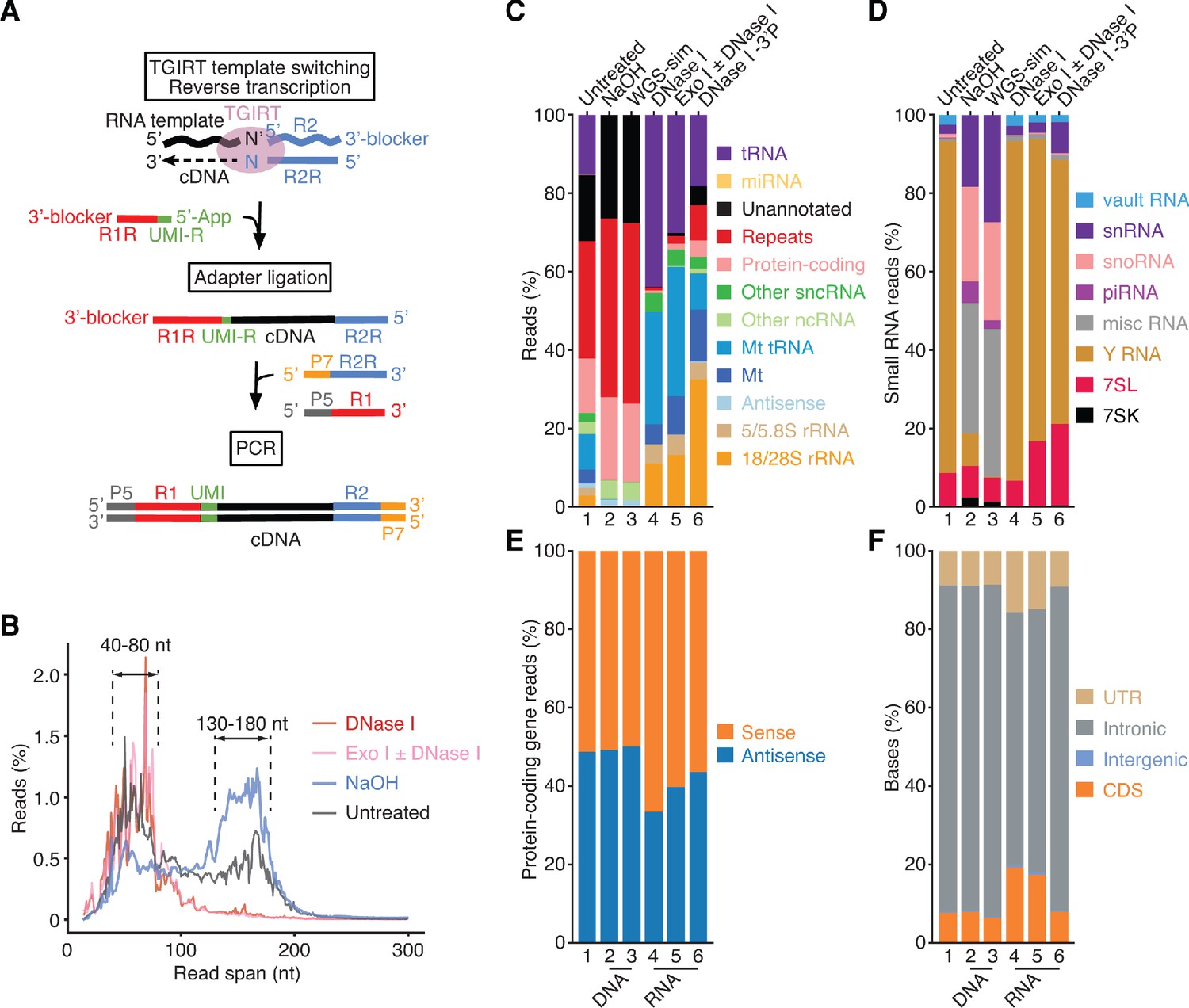
(A) TGIRT-seq workflow. The TGIRT enzyme initiates reverse transcription by template switching from a synthetic RNA template/DNA primer substrate consisting of a 35-nt RNA oligonucleotide containing an Illumina read 2 (R2) sequence annealed to a 36-nt DNA primer. The latter leaves a single nucleotide 3’ overhang (N, an equimolar mix of A, C, G, and T) that directs template switching by base pairing to the 3’ nucleotide (N’) of an RNA or DNA template, which is then reverse transcribed resulting in a DNA copy of the nucleic acid with the reverse complement of an Illumina read two sequence (R2R) seamlessly linked to its 5’ end (Qin et al., 2016; Wu and Lambowitz, 2017). After clean-up, a second adapter (R1R DNA), which contains the reverse complement of an Illumina read one sequence and introduces a 6-nt UMI (denoted UMI-R for the reverse orientation), is ligated to the 3’ end of the cDNA using thermostable 5’ App DNA/RNA ligase, followed by PCR with primers that add capture sites and indices for Illumina sequencing. (B) Read-span distributions in combined datasets for plasma nucleic acids before (n = 3) and after treatment with NaOH to digest RNA (n = 4) or with DNase I (n = 12) or Exonuclease I (Exo I) ± DNase I (n = 3) to digest DNA. The plot shows the percentage of read spans as a function of length calculated from the starting positions of each deduplicated 2 × 75 nt paired-end read. (C) and (D) Stacked bar graphs showing the percentage of deduplicated read pairs in the indicated combined datasets that mapped to different categories of annotated genomic features or unannotated regions of the hg19 human genome reference sequence compared to a simulated dataset of 2 × 75 nt paired-end reads (WGS-sim) generated computationally from the hg19 sequence. Genomic features follow Ensembl annotations. Mt indicates mitochondrial transcripts, and Repeats indicates Repbase-annotated repeats. Other ncRNA includes pseudogenes and Ensembl-annotated long non-coding RNAs (lncRNAs). Other sncRNA indicates the small non-coding RNAs classified by Ensembl and broken out separately in panel (D). (E) Stacked bar graphs showing the percentages of reads that mapped to the sense or antisense strand of protein-coding genes. Strand specificity was calculated after filtering out read pairs that aligned to embedded sncRNAs, such as snoRNAs, but included read pairs that aligned to repeats within protein-coding genes. (F) Stacked bar graphs showing the percentage of bases that mapped to different regions of the sense strand of protein-coding genes. UTR, 5’- or 3’-untranslated region; CDS, coding sequences; intergenic, regions upstream or downstream of transcription start and stop sites annotated in RefSeq. In panels (C)-(F), features are color-coded as indicated in the Figure, and numbers at the bottom indicate the same samples with different categorizations.
Figure 1—figure supplement 1
Bioanalyzer traces of plasma nucleic acids before and after various treatments.
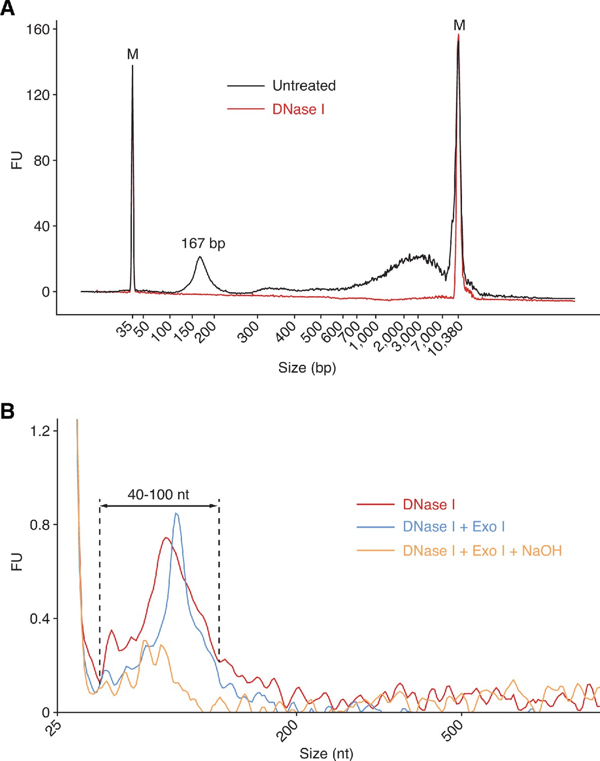
Nucleic acids were extracted from plasma with a QIAamp ccfDNA/RNA kit and analyzed by using an Agilent 2100 Bioanalyzer. (A) Plasma nucleic acid samples before and after treatment with DNase I to digest DNA analyzed by using a High Sensitivity DNA kit, which detects only dsDNA. The traces show a major DNase I-sensitive peak at 167 bp corresponding to chromatosome/nucleosome-protected DNA (Wu and Lambowitz, 2017), along with larger material, which may correspond to DNA from oligonucleosomes or damaged DNA that runs anomalously on the Bioanalyzer. (B) Plasma RNA samples after different treatments to remove DNA analyzed with an RNA 6000 Pico kit. The traces show peaks between 40 and 100 nt that are largely sensitive to NaOH. FU indicates arbitrary fluorescent units reported by the Bioanalyzer software.
Figure 1—figure supplement 2
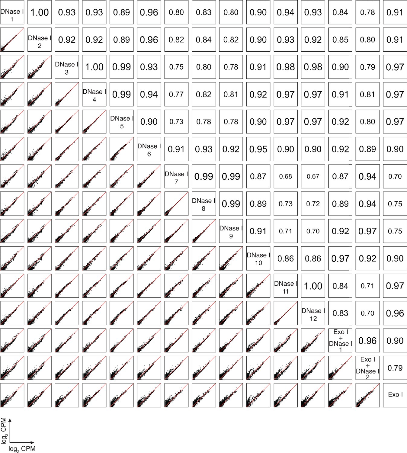
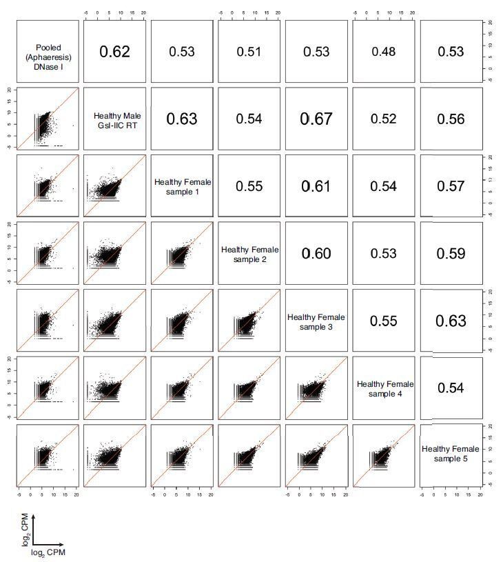
Correlation matrix for individual datasets of plasma RNA after different DNA-removal treatments: DNase I (n = 12) and Exo I ± DNase I (n = 3).
For comparisons, CPMs for each gene in a dataset were normalized to the total number of mapped reads in that dataset, log2 transformed, and plotted. Pearson correlation coefficients are shown on the upper triangle. Numbers on the x and y axes of scatter plots are log2 transformed CPMs.
Figure 1—figure supplement 3
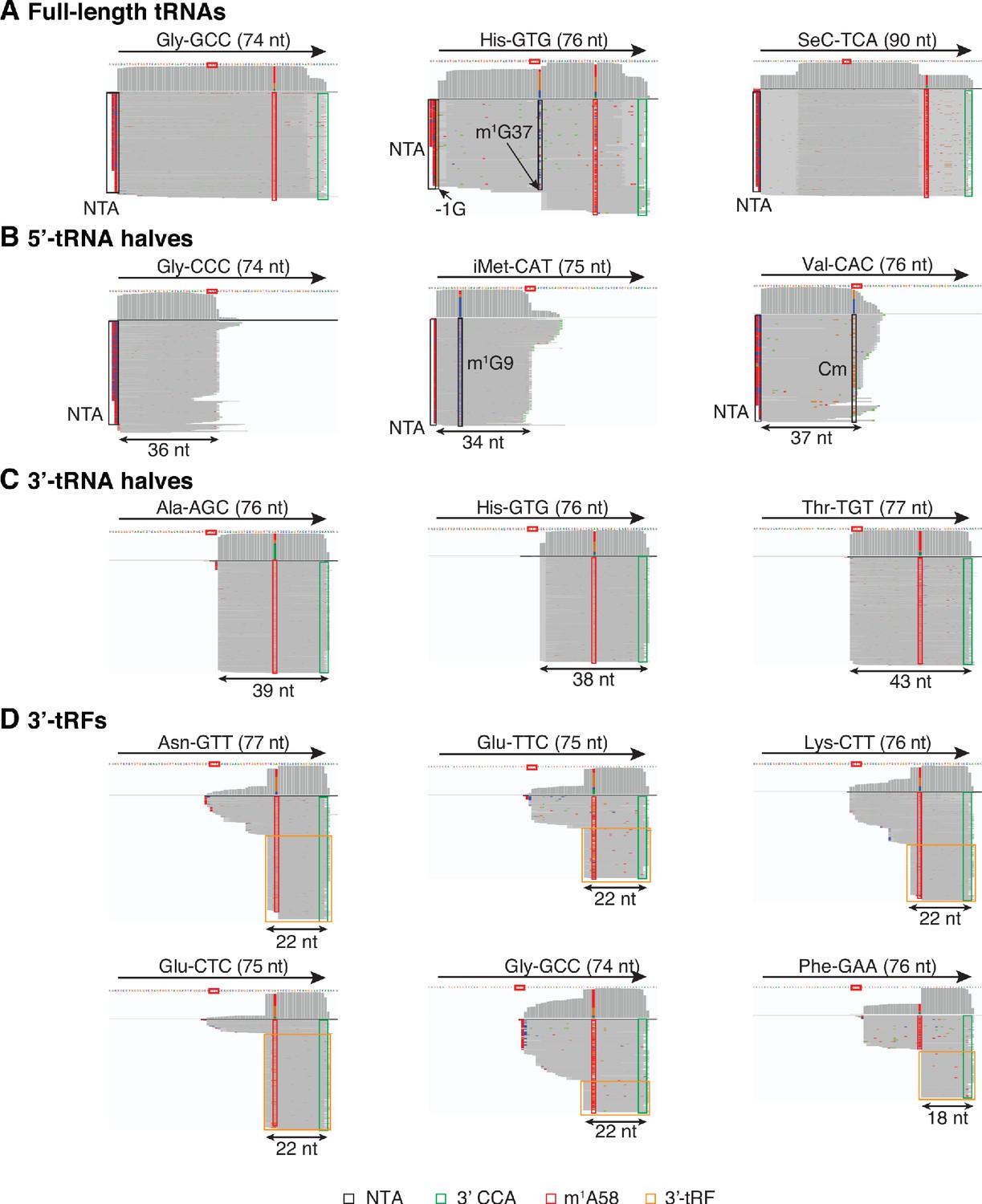
IGV screenshots showing examples of full-length mature tRNAs and tRNA fragments detected in plasma by TGIRT-seq.
(A) Full-length mature tRNAs; (B) 5'-tRNA halves; (C) 3'-tRNA halves; and (D) 3'-tRFs. The tRNA name and length are indicated at the top, with an arrow indicating the 5' to 3' orientation, and the tRNA sequence with anticodon positions boxed in red shown below. The IGV coverage plots and alignments below the tRNA sequence were generated from combined datasets for DNase I-treated plasma RNA (n = 12) mapped to mature tRNA reference sequences containing a 3' CCA tail (Chan and Lowe, 2016). Coverage at each position along the gene is shown in the top track, and read alignments are shown below with reads down sampled to a maximum of 100 reads for display when necessary. Gray represents bases that match the reference base. Other colors indicate bases that do not match the reference base (red, green, blue, and brown indicate thymidine, adenosine, cytidine, and guanosine, respectively). Misincorporation at known sites of post-transcriptionally modified bases are highlighted in the alignments: red boxes, m1A58: 1-methyladenosine at position 58; black boxes, m1G37 in His-GTG, m1G9 in iMet-CAT, Cm (2’O-methylation of ribose at C34) in Val-CAC, and −1G in His-GTG. Because tRNA halves and tRFs are much less abundant than mature tRNAs, for visualization in panels B-D, only read pairs with read span < 50 nt and a 3'-RNA end mapping to the anticodon loop are shown for 5’-tRNA halves, and only read pairs with a read span < 50 nt and ending with a 3'-CCA tail are shown for 3'-tRNA halves and 3'-tRFs. Reads corresponding to 3’-tRFs are in orange boxes, and 3’ CCAs are in green boxes. NTA/black boxes are non-templated nucleotides added by TGIRT-III to the 3' end of cDNAs (5' end of the RNA sequence) during TGIRT-seq library preparation.
Figure 1—figure supplement 4
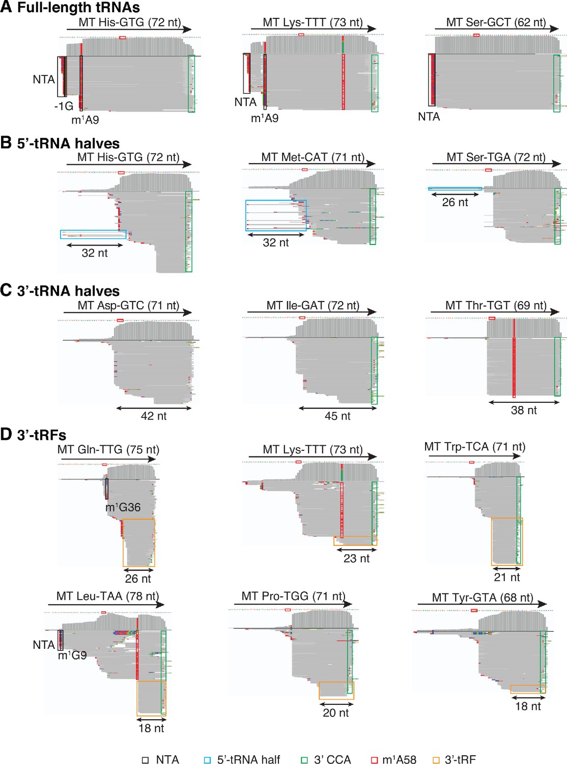
IGV screenshots showing examples of full-length mitochondrial (Mt) tRNAs and tRNA fragments.
(A) Full-length mature tRNAs; (B) 5'-tRNA halves; (C) 3'-tRNA halves; and (D) 3'-tRFs. IGV screen shots were generated from combined datasets for DNase I-treated plasma RNA (n = 12) and labeled as described in Figure 1—figure supplement 3. Misincorporation at known sites of post-transcriptionally modified bases are highlighted in the read alignments: red boxes, m1A58: 1-methyladenosine at position 58; black boxes, m1G36 in Gln-TTG, m1G9 in Leu-TAA, m1A9 in His-GTG and Lys-TTT, and −1G in His-GTG. NTA Reads corresponding to 5’-tRNA halves are in light blue boxes, and reads corresponding to 3’-tRFs are in orange boxes.
Figure 1—figure supplement 5
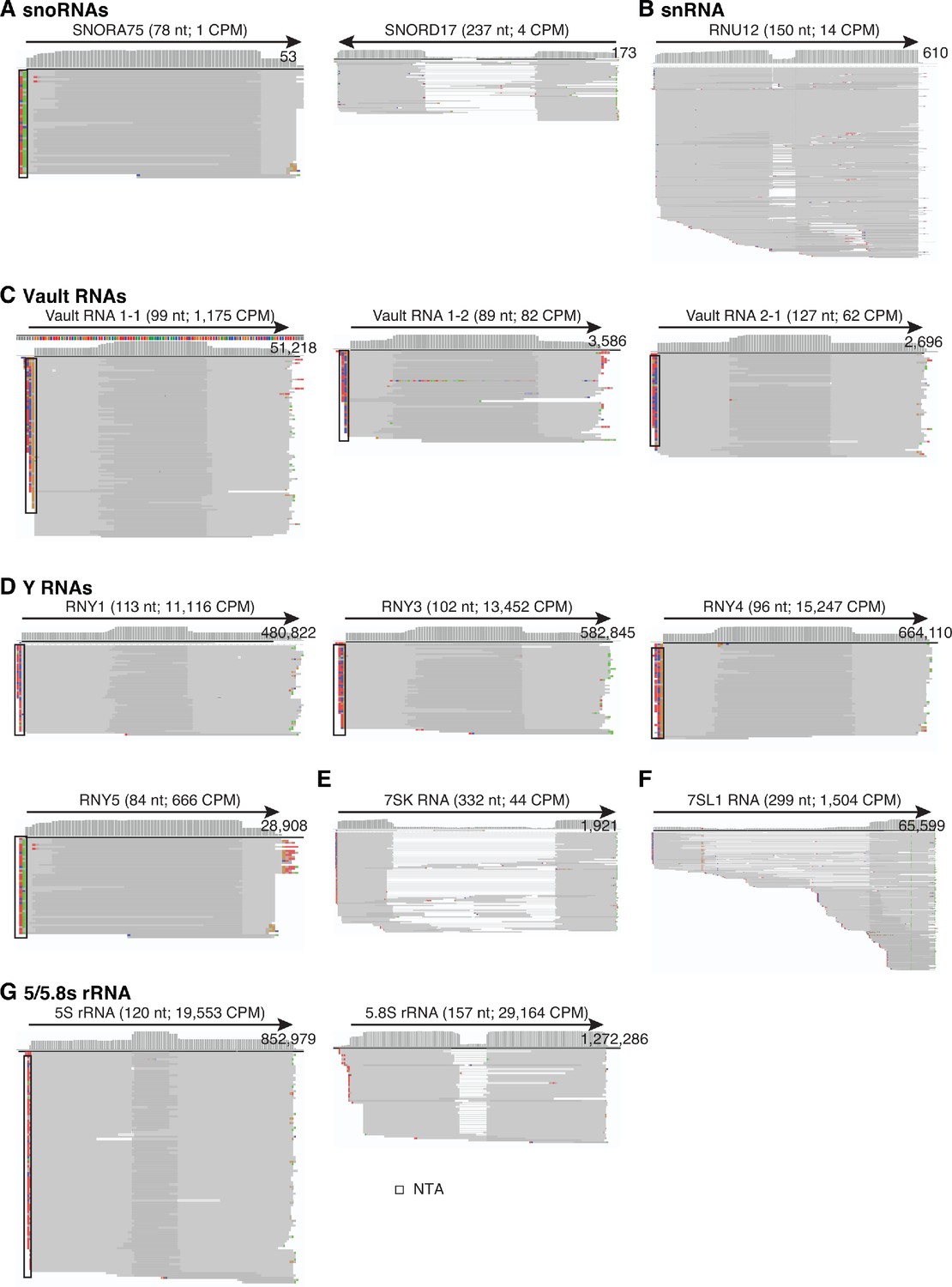
IGV screenshots showing examples of sncRNAs detected in combined datasets for DNase I-treated plasma RNA samples (n = 12).
The name of the RNA is indicated at the top with the length (nt) and counts per million (CPM) for deduplicated reads shown in parentheses. The arrow below indicates the 5’ to 3’ orientation of the RNA. IGV coverage plots and alignments are labeled as described in Figure 1—figure supplement 3, with reads in the alignment down sampled to a maximum of 100. (A) The two most highly abundant snoRNAs (SNORA75 and SNORD17); (B) snRNA (RNU12); (C) Vault RNAs (Vault RNAs 1–1, 1–2, and 2–1); (D) Y RNAs (RNY1, RNY3, RNY4 and RNY5); (E) 7SK RNA; (F) 7SL RNA; and (G) 5S and 5.8S rRNA. In the read alignments, overlapping regions of paired-end reads are darker gray, and non-overlapping read pairs for RNAs > 150 nt (e.g., 7SK and SNORD17) are shown as gaps connected by thin blue lines. NTA/black boxes are non-templated nucleotides added during TGIRT-seq library preparation.
Figure 1—figure supplement 6
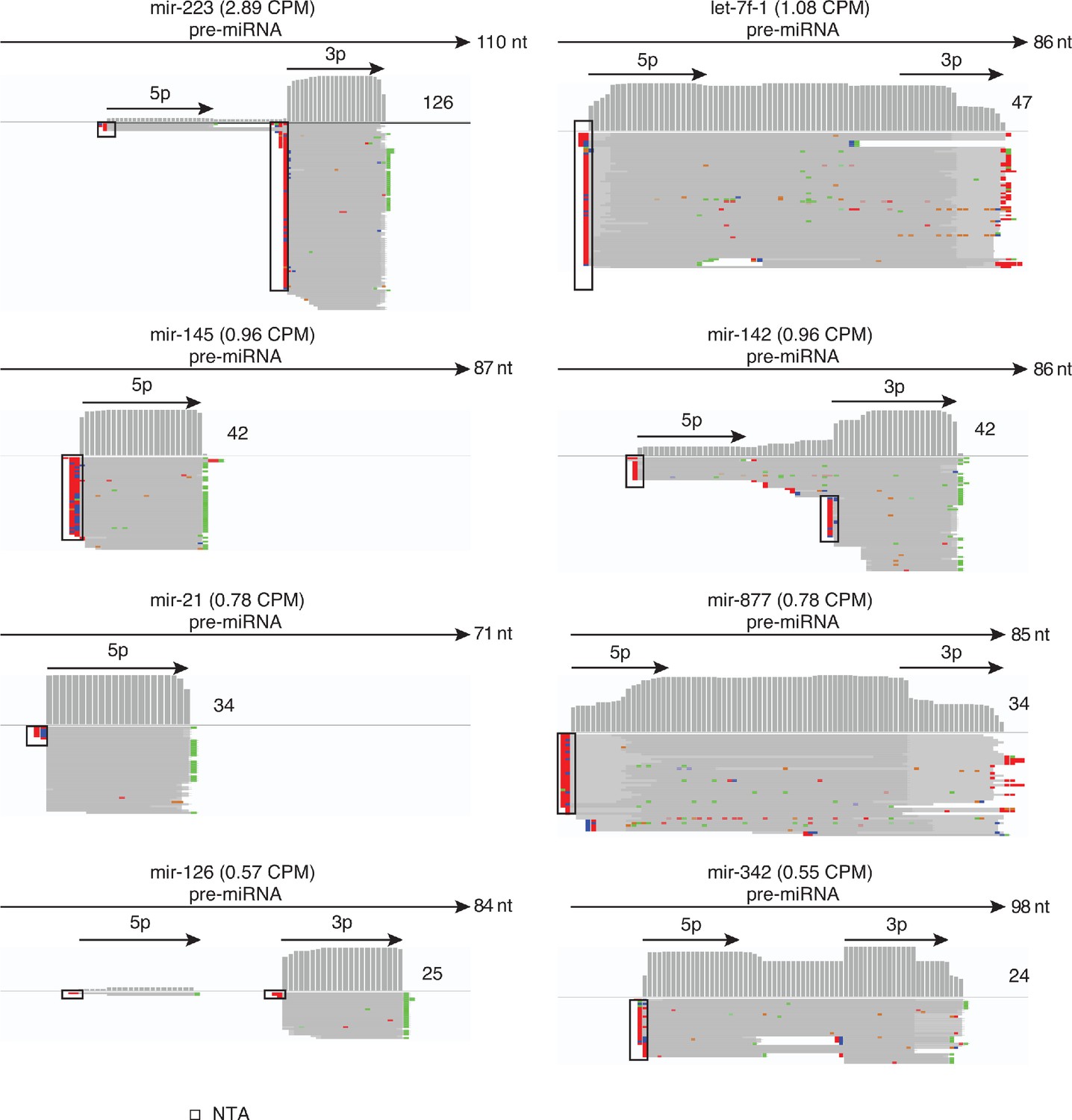
Human plasma contains different miRNA isoforms.
The Figure shows IGV screen shots of examples from the top 15 most abundant miRBase-validated miRNAs in combined datasets for DNase I-treated plasma RNA (n = 12). The miRNA name is indicated at the top with CPM values for all mapped deduplicated reads indicated in parentheses. The arrows below correspond to the annotated pre-miRNA and its 5 p and 3 p segments, with the length of the pre-miRNA indicated to the right of the arrow. IGV coverage plots and alignments are shown below, labeled as in Figure 1—figure supplement 3, with the number of deduplicated reads indicated to the right of the coverage plot. Reads shown in the alignment were down sampled to 100 reads when necessary for display. NTA/black boxes are non-templated nucleotides added during TGIRT-seq library preparation.
Figure 2
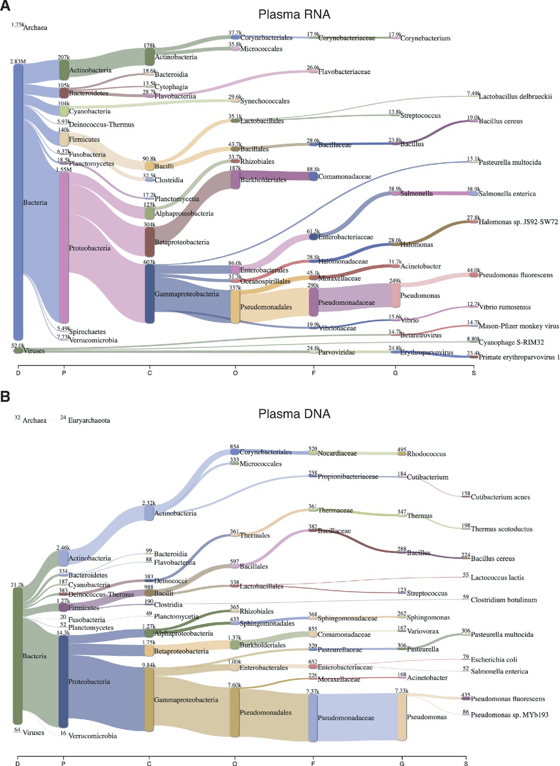
Sankey diagram of reads assigned to bacteria, archaea, and viruses from combined datasets of (A) DNase-treated plasma RNA (n = 15) and (B) NaOH-treated plasma DNA (n = 4).
The diagram shows the flow of mapped reads from the most general (left) to most specific (right) taxonomic classification (abbreviations: D, Domain; P, Phylum; C, Class; O, Order; F, Family; G, Genus; S, Species). The width of the flow is proportional to the number of reads, which is indicated at the top of each node.
Figure 3 with 2 supplements
TGIRT-seq analysis of protein-coding gene transcripts in human plasma and comparison with SMART-Seq.
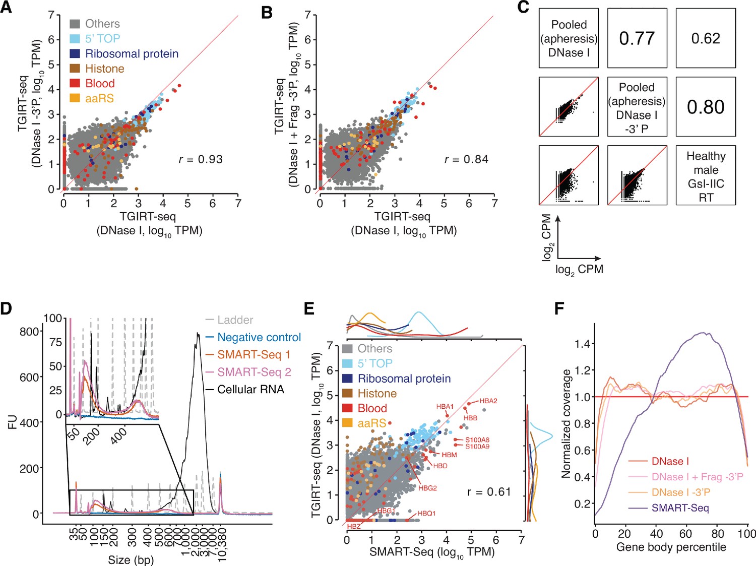
(A, B) Scatter plots comparing protein-coding gene transcripts detected by TGIRT-seq in combined datasets for DNase I-treated plasma RNA without (n = 12) or with (n = 3) 3'-phosphate removal or chemical fragmentation followed by 3'-phosphate removal (n = 5). Reads aligned to protein-coding genes were extracted and quantified by Kallisto to obtain transcript-per-million (TPM) values, and average TPM values for each gene were plotted for each pairwise comparison. Each point represents one gene and is color-coded by type of encoded protein as indicated in the Figure. 5’ TOP includes those ribosomal proteins whose mRNAs have a 5' TOP sequence. The red line indicates identical TPM values for both methods. Pearson correlation coefficients are shown at the lower right. (C) Scatter plots comparing the relative abundances of protein-coding gene transcripts detected in DNase I-treated plasma RNA using the improved TGIRT-seq method in this work without (n = 12) or with (n = 3) 3'-phosphate removal with those detected previously by TGIRT-seq in DNase I-treated plasma RNA from a healthy male individual (n = 3; SRP064378, datasets 12–14) (Qin et al., 2016). CPMs for each gene were normalized to the total number of mapped reads in the dataset and log2 transformed for the comparisons. Spearman correlation coefficients are shown in sectors at the upper right. (D) Bioanalyzer traces of PCR-amplified cDNAs generated by SMART-Seq according to manufacturer’s protocol. Samples were analyzed using an Agilent 2100 Bioanalyzer with a High Sensitivity DNA kit. Traces are color-coded by sample type as shown in the Figure, with ‘Ladder’ (dashed gray lines) indicating the DNA ladder supplied with the High Sensitivity DNA kit. The negative control was a SMART-Seq library prepared with water as input, and the cellular RNA control was the positive control RNA supplied with the SMART-Seq kit. SMART-Seq 1 and 2 indicate double-stranded DNAs generated by using the SMART-Seq kit from different samples of DNase I-treated plasma RNA. FU, fluorescence units. (E) Scatter plot comparing protein-coding gene transcripts detected in plasma by TGIRT-seq and SMART-Seq. Reads assigned to protein-coding genes transcripts (0.28 million reads for TGIRT-seq and 2.6 million reads for SMART-Seq) were extracted from combined datasets obtained from DNase I-treated plasma RNA (n = 12 for TGIRT-seq and n = 4 for SMART-Seq) and quantified by Kallisto. The scatter plots compare average TPM values for protein-coding gene transcripts with each point representing one gene, color-coded by the type of encoded protein (see above). The marginal distributions of different color-coded mRNA species in the scatter plot are shown above for SMART-Seq and to the right for TGIRT-seq. The red line indicates identical TPM values for both methods. The Pearson correlation coefficient (r) is indicated at the bottom right. (F) Normalized 5’- to 3’-gene body coverage for protein-coding gene transcripts detected in plasma by TGIRT-seq and SMART-Seq. Gene body coverage was computed by Picard tools (Broad Institute) using the genomic alignment files generated by Kallisto. The plots show normalized gene coverage versus normalized gene length for all protein-coding transcripts in the indicated datasets color-coded as indicated in the Figure. The red horizontal line at y = 1 indicates perfectly uniform 5' to 3' coverage.
Figure 3—figure supplement 1
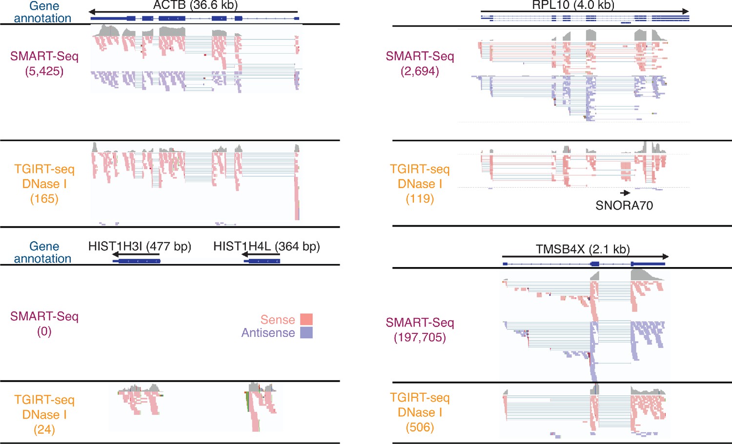
IGV screen shots showing examples of protein-coding gene transcripts detected in DNase I-treated plasma RNA by SMART-Seq and TGIRT-seq.
The gene name and length are indicated at the top with the arrow below indicating the 5' to 3' orientation of the mRNA. The gene model from RefSeq is shown below (exons, blue bars; introns, thin blue lines). Coverage tracks (gray) for the combined SMART-Seq and TGIRT-seq datasets are shown below the gene model followed by read alignments for the sense (pink) and antisense (purple) orientations down sampled to 100 reads for display when necessary. Colors other than pink or purple in the read alignments indicate bases that do not match the reference sequence (red, green, blue, and brown indicate thymidine, adenosine, cytidine, and guanosine, respectively). Spliced exons are connected by thin blue lines. The IGV alignment for ribosomal protein gene RPL10 shows an embedded snoRNA (SNORA70) that is detected by TGIRT-seq but not by SMART-Seq.
Figure 3—figure supplement 2
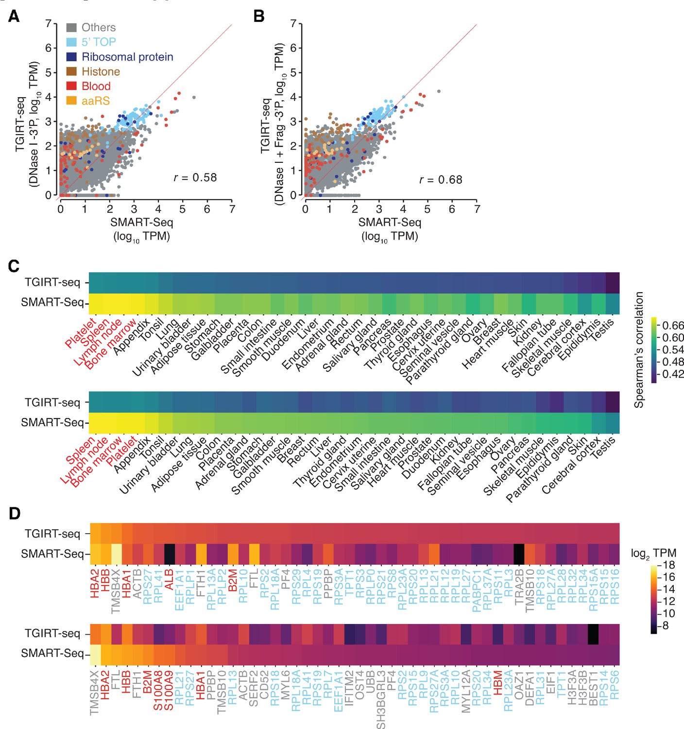
Additional scatter plots and heat maps comparing protein-coding gene transcripts detected in DNase I-treated plasma RNA by TGIRT-seq and SMART-Seq.
(A, B) Scatter plots comparing the relative abundances of protein-coding gene transcripts detected in DNase I-treated plasma RNA in combined SMART-Seq datasets (n = 4) with those in combined TGIRT-seq datasets for DNase I-treated plasma RNA with 3'-phosphate removal (n = 3) or with chemical fragmentation followed by 3'-phosphate removal (n = 4), respectively. Data were processed as described for Figure 3A and B. (C) Heat maps comparing protein-coding gene transcripts detected by TGIRT-seq or SMART-Seq to primary tissue transcriptomic data obtained from the Human Protein Atlas (Uhlén et al., 2015) and platelet transcriptomic data obtained from Campbell et al., 2018. Primary tissues are ranked in descending order by Spearman correlation values from combined TGIRT-seq (top) or SMART-Seq (bottom) datasets. The names of blood-related tissues are in red. (D) Heat map of log2 TPM values for the top 50 most abundant protein-coding gene transcripts detected by TGIRT-seq (top panel) and SMART-Seq (bottom panel). The transcripts are shown in descending order of TPM values quantified by Kallisto, with the gene names color-coded as indicated in panel A.
Figure 4 with 3 supplements
Peak-calling analysis of plasma RNA.
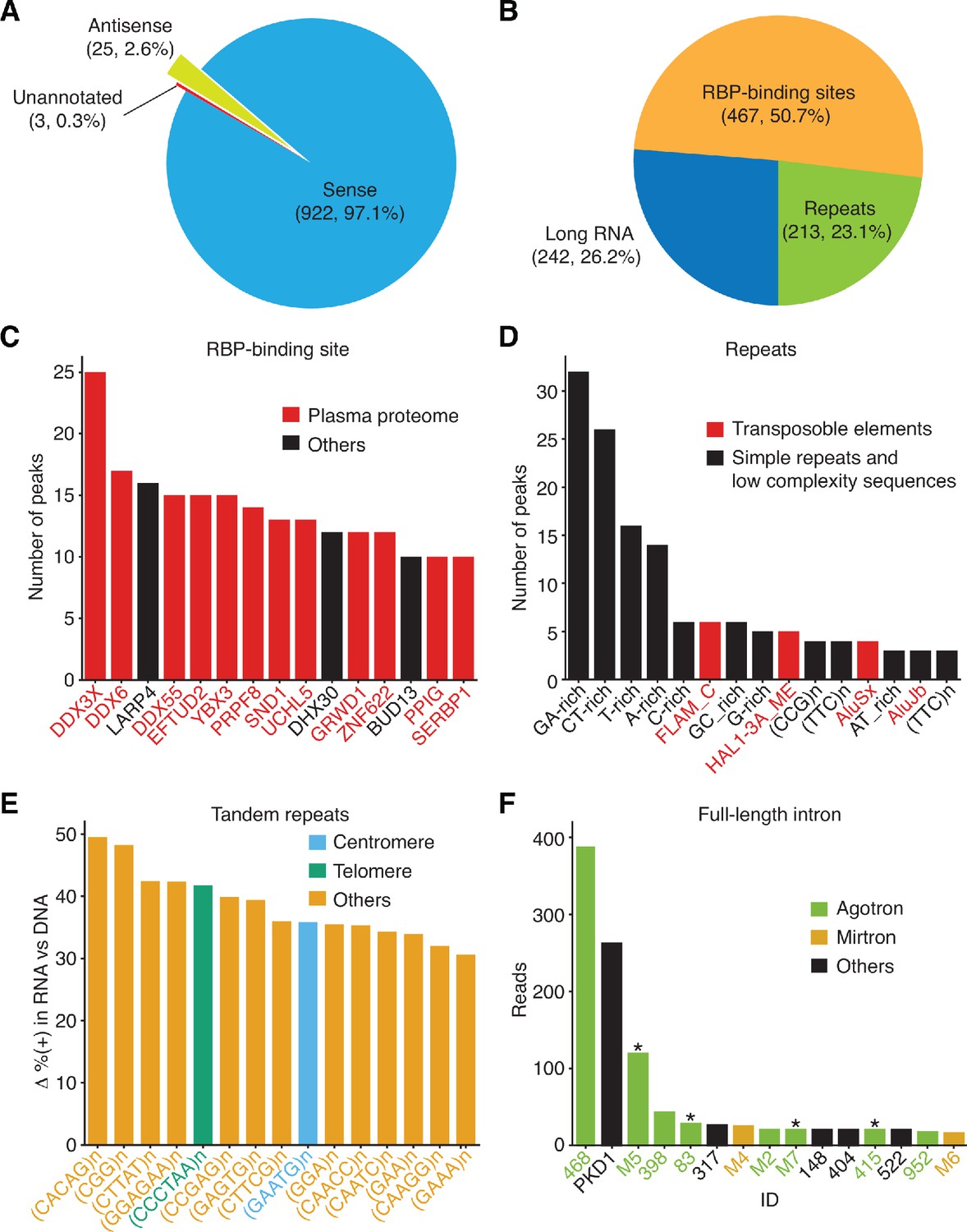
The MACS2 algorithm was used to call peaks in combined TGIRT-seq datasets for DNase-treated plasma RNA (n = 15) after removal of the reads for rRNAs, Mt RNAs, and annotated sncRNAs (tRNAs, Y RNAs, 7SK and 7SL RNAs, vault RNAs, snoRNAs, snRNAs, high confidence miRNAs, and miscellaneous RNAs). The combined datasets for NaOH-treated plasma DNA (n = 4) were used as the base-line control. Only peaks with q-value < 0.05 assigned by MACS2 and supported by alignments from at least five separate libraries at the peak summit were used for the analysis. Peaks were intersected sequentially with (i) binding sites for 109 RNA-binding protein (RBPs) from ENCODE K-562 and HepG2 cell eCLIP datasets; (ii) RefSeq and GENCODE gene annotations; and (iii) repeat annotations from Repbase, and a best feature annotation for each peak was selected by the highest overlap score, as described in Materials and methods. (A) and (B) Pie charts showing the proportion of peaks with annotations on the sense strand, antisense strand, or no annotations (A) and the proportion of peaks mapping to different categories of genomic features with sense-strand annotations (B). The number of peaks in each sector and their percentage of the total are indicated in parentheses. (C–F) Bar graphs showing the (C) top 15 RBP-binding sites ranked by peak count, with RBPs found to be part of the plasma proteome (Nanjappa et al., 2014) shown in red; (D) top 15 Repbase annotated repeats ranked by peak count, with simple repeats and low complexity sequences in black and transposable element RNAs in red; (E) top 15 short tandem repeat RNAs with highest difference (Δ) in the percentage of (+) orientation reads between the DNase-treated plasma RNA and NaOH-treated plasma DNA datasets color coded as indicated in the Figure; (F) top 15 peaks corresponding to full-length excised intron RNAs ranked by the number of deduplicated reads. The peak IDs are indicated on the x-axis and are color-coded by annotated intron RNA type: agotron (green); mirtron (gold); annotated as both agotron and mirtron (green with asterisk). Others, not annotated in the previous categories (black). The read count for PKD1 is the combined count from the peak in PKD1 gene and the peaks for the same intron in six PKD1 pseudogenes (Figure 9D below and peak IDs #335–340).
Figure 4—figure supplement 1
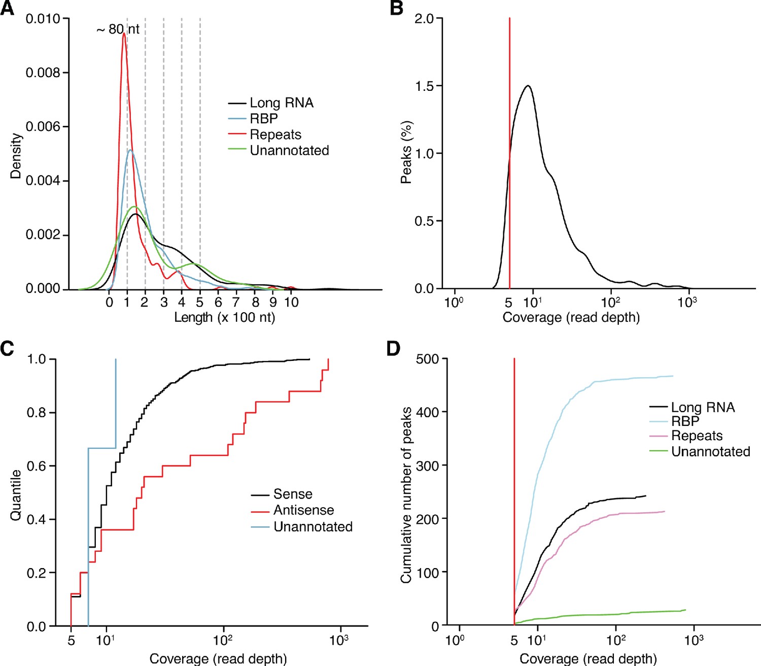
Characteristics of different categories of peaks identified by MACS2 peak calling analysis of combined datasets of DNase-treated plasma RNA (n = 15).
(A) Density plot showing the range of peak lengths computed from the genomic positions at the beginning and end of each peak. (B) Distribution plot of the number of reads mapping within the called peaks. (C) Empirical cumulative distribution plots of read coverage for different categories of peaks. Peaks that overlapped annotated features on the sense strand were classified as ‘Sense’; peaks on the antisense strand that overlapped annotated sense-strand feature were classified as ‘Antisense’; and the remainder of the peaks were classified as ‘Unannotated’. (D) Cumulative peak count with increasing coverage threshold. Plots are color-coded by peak type as indicated in the Figure. In panels (B) and (D), the red vertical line represents the coverage cutoff for significant peaks (coverage ≥ 5 deduplicated reads).
Figure 4—figure supplement 2
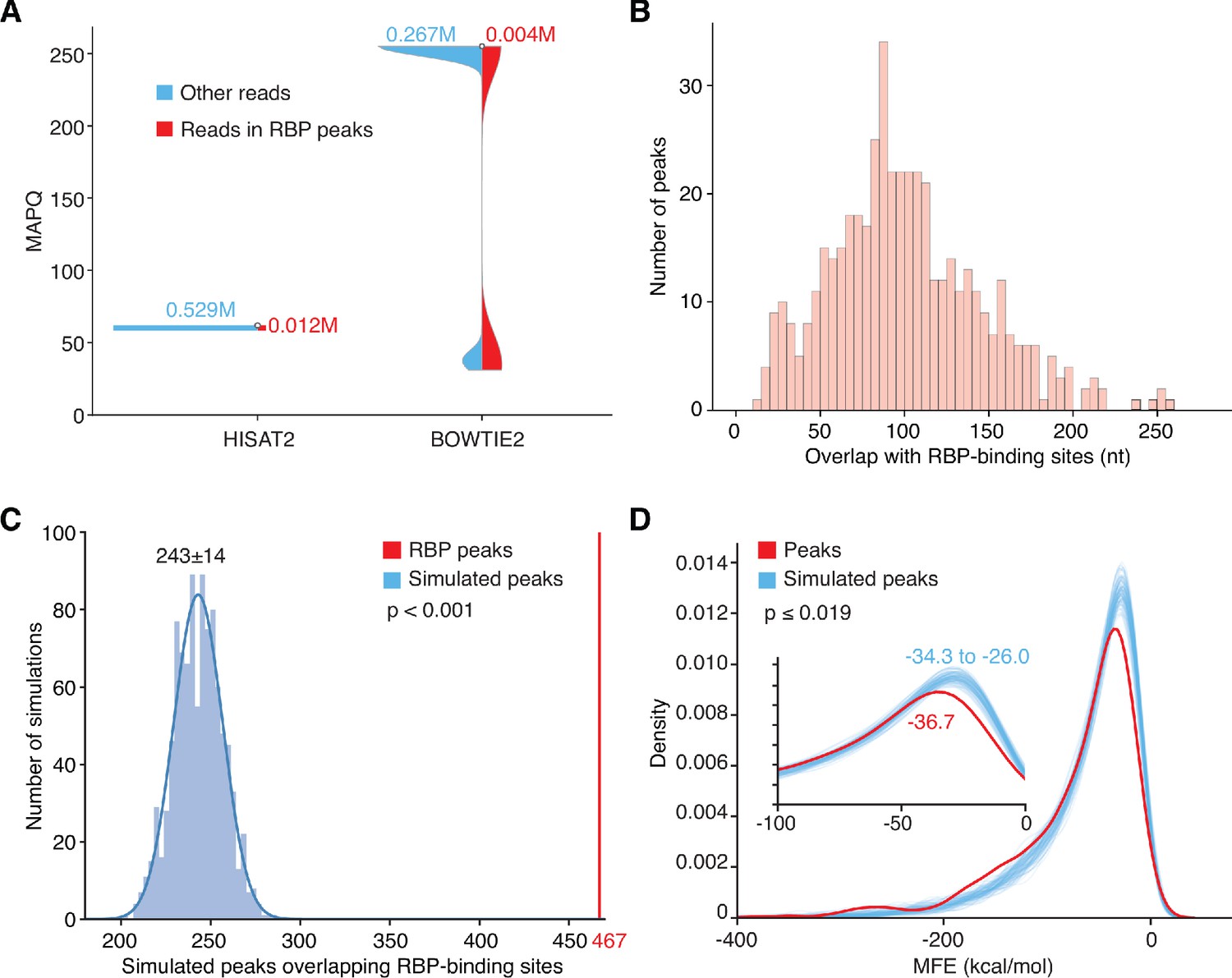
Overlap, quality control, and statistical significance of MACS2-called peaks corresponding to annotated RBP-binding sites.
(A) Violin plots of mapping quality (MAPQ) scores for reads in peaks corresponding to RBP-binding sites compared to other long RNA reads with MAPQ ≥ 30, the cutoff for BOWTIE2-mapped reads used in peak calling. HISAT2 and BOWTIE2 use different methods for calculating MAPQ. Reads uniquely mapped by HISAT2 have MAPQ = 60; reads uniquely mapped by BOWTIE2 have MAPQ = 255; and reads mapped to multiple loci by BOWTIE2 have lower MAPQ scores. The MAPQ cutoff of ≥ 30 eliminates BOWTIE2 mapped reads that mapped equally well to more than one locus. (B) Histogram of the number of overlapping nucleotides between the called peaks and annotated-RBP-binding sites in the ENCODE eCLIP datasets. (C) Histogram of the number of simulated peaks overlapping RBP binding sites in 1000 repeat simulations using peaks randomly generated from the sequences of genes encoding long RNAs. In the simulations, 950 peaks with the same size distribution as the 950 high confidence peaks called by MACS2 were randomly generated from the sequences of the genes encoding all long RNAs detected in the combined DNase-treated plasma RNA datasets (n = 15) and checked for overlap with the binding sites for 109 RBPs in the ENCODE eCLIP datasets. In 1,000 repeats of the simulation, the simulated peaks overlapped 201 to 287 RBP-binding sites by chance compared to 467 RBP-binding sites for the plasma RNA peaks called by MACS2 (red vertical line). The simulations indicate that the enrichment of RBP-binding sites in the called RNA peaks is statistically significant (p-value < 0.001). (D) Density plots of the calculated MFEs of the most stable RNA secondary structure predicted by RNAfold for the 709 high confidence long RNA peaks called by MACS2 (467 RBP-binding protein and 242 non-RBP-binding protein peak; red) compared to 709 simulated peaks (blue) with the same size distribution randomly generated from the sequences of genes encoding all long RNAs detected in the combined DNase-treated plasma RNA datasets (n = 15). One hundred repeats of the simulation indicated that the higher predicted stabilities (lower predicted MFEs) of the called long RNA peaks is statistically significant (p-value ≤ 0.019).
Figure 4—figure supplement 3
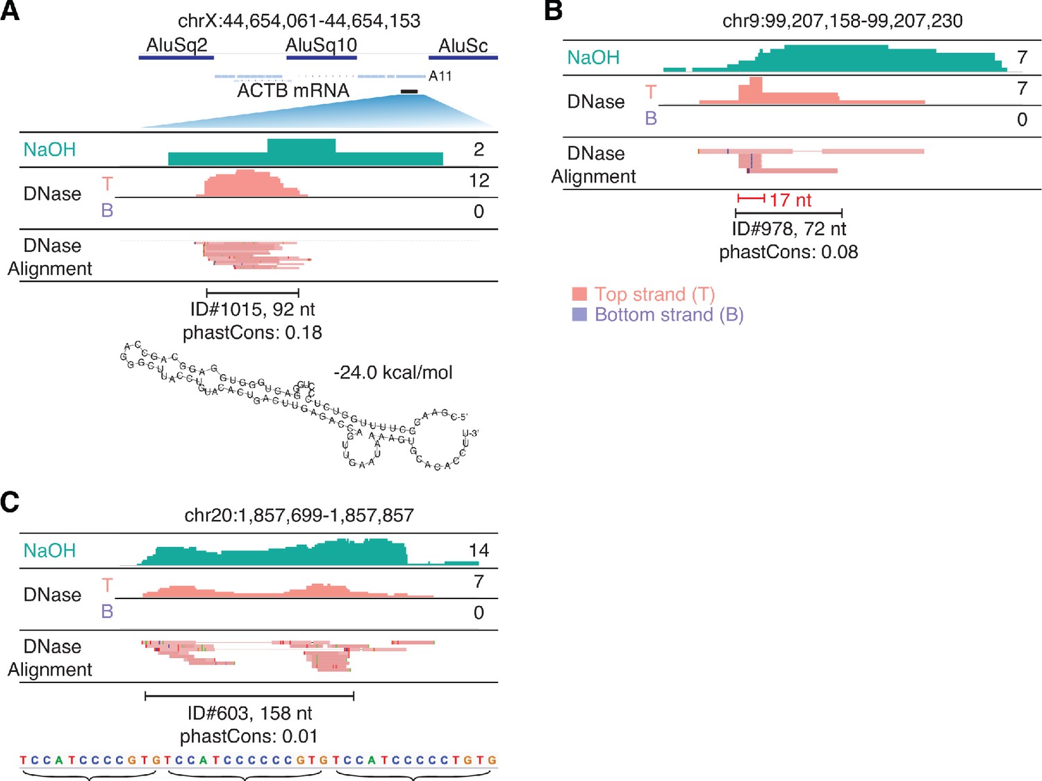
IGV screenshots showing peaks mapping to unannotated genomic loci.
The hg19 genomic coordinates of the called peak are indicated at the top, and IGV alignments labeled as in Figure 9 are shown below. Peaks are delineated by a bracketed black line, with peak ID number, length, and phastCons scores for 46 vertebrates indicated below. (A) A peak corresponding to a segment of a retrotransposed mRNA with a short poly(A) tail (A11). The retrotransposed mRNA sequence (blue line) is flanked by two Alu elements and has an internal Alu element insertion. The segment of the mRNA sequence corresponding to the peak (black bar) is expanded for the IGV alignments. The most stable predicted secondary structure and its MFE (ΔG) computed by RNAfold are shown below. (B) A peak containing a short (17 nt) RNA with discrete 5' and 3' ends (bracketed red line) (C) A peak containing reads with heterogenous 5' and 3' ends containing tandem repeats of the sequence indicated below.
Figure 5
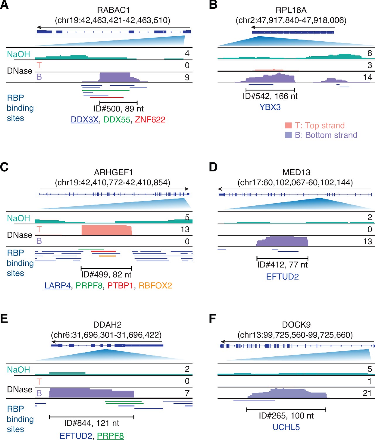
Integrative Genomics Viewer (IGV) screenshots showing examples of plasma RNA peaks corresponding to annotated RBP-binding sites detected in plasma by TGIRT-seq peak calling.
(A–F) Gene names are indicated at the top with the hg19 coordinates of the called peak in parentheses and an arrow below indicating the 5’ to 3’ orientation of the encoded RNA. The top track shows the gene map (exons, thick bars; intron, thin lines), with the relevant part of the gene map expanded below. The tracks below the gene map show coverage plots for the peak region in combined datasets for NaOH-treated plasma DNA (n = 4; combined top and bottom strands, turquoise) or DNase-treated plasma RNA (n = 15; Top strand (T), pink and Bottom strand (B), purple) based on the number of deduplicated reads indicated to the right. The peak called by MACS2 is delineated by the bracketed line, with the peak ID and length indicated below. Annotated protein-binding sites are shown as color-coded lines below the coverage plots. For cases in which the peak overlaps multiple RBP-binding sites, the one whose annotated binding site had the largest number of bases overlapping the peak is underlined.
Figure 6 with 1 supplement

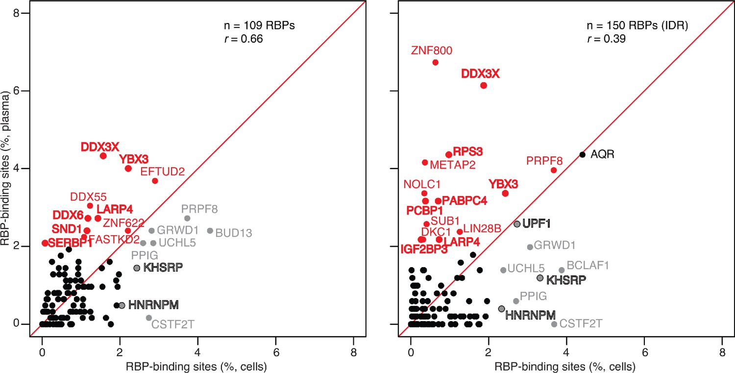
Scatter plot comparing the relative abundances of RBP-binding sites in plasma RNA peaks called against the human genome reference sequence with those of RBP-binding sites in ENCODE eCLIP cellular RNA datasets (ENCODE 109 RBP eCLIP dataset on the left and 150 RBP eCLIP dataset with irreproducible discovery rate (IDR) analysis on the right; the RBPs whose binding sites were searched are listed in the Supplementary file 1).
Abundant RBP-binding sites enriched in plasma or cellular RNAs are indicated in red and gray, respectively. Stress granule proteins are indicated in bold. r is the Pearson correlation coefficient.
Figure 6—figure supplement 1
Scatter plot comparing the relative abundances of RBP-binding sites in plasma RNA peaks called against both the human genome and transcriptome reference sequences with those of RBP-binding sites in ENCODE eCLIP cellular RNA datasets (ENCODE 109 RBP eCLIP dataset on the left and 150 RBP eCLIP dataset with irreproducible discovery rate (IDR) analysis on the right; the RBPs whose binding sites were searched are listed in the Supplementary file 1).
Abundant RBP-binding sites enriched in plasma or cellular RNAs are indicated in red and gray, respectively. Stress granule proteins are indicated in bold. r is the Pearson correlation coefficient.
Figure 7 with 3 supplements
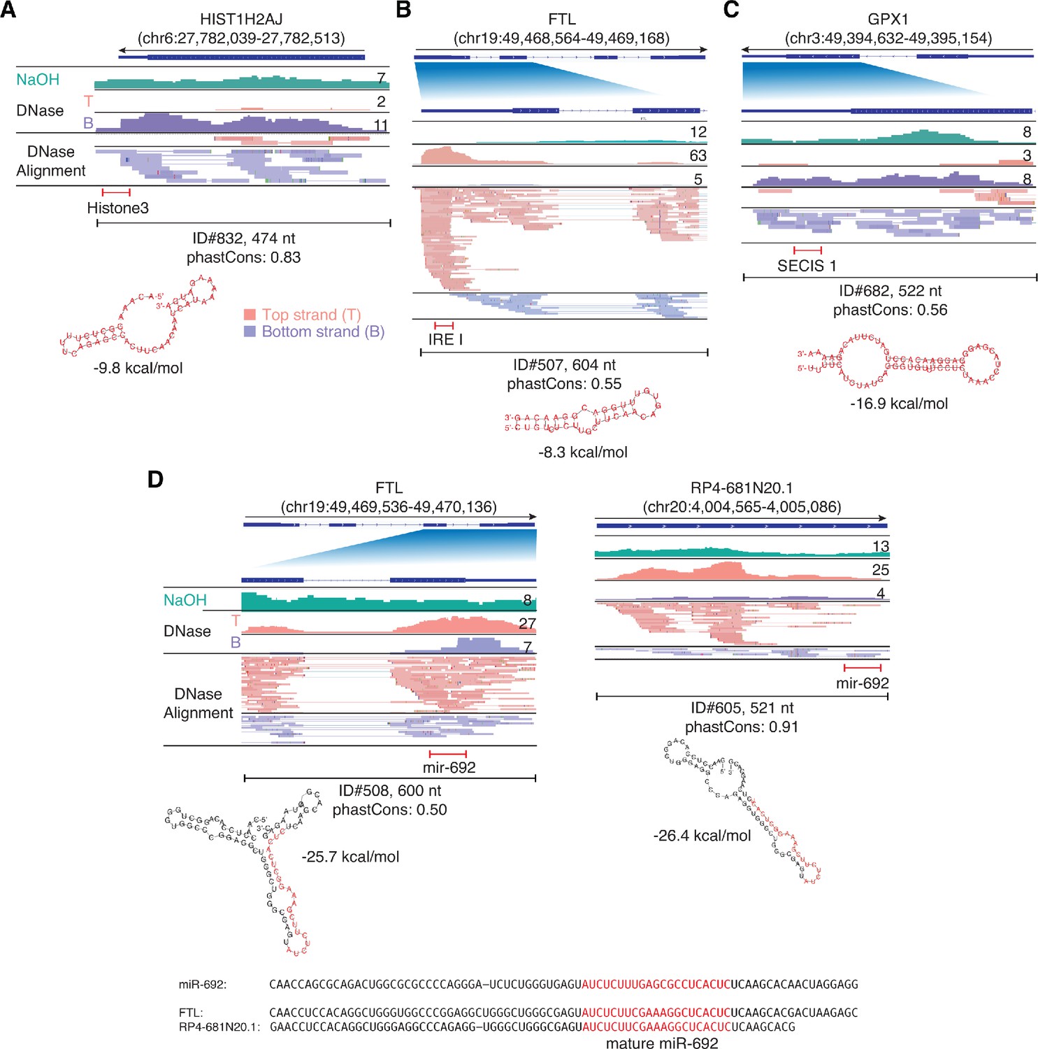
IGV screenshots showing examples of peaks mapping to exons or pseudogenes that contain regions classified by Infernal/Rfam (Kalvari et al., 2018) as belonging to known classes of structured RNAs.
(A) A segment of peak near the 3’ end of HIST1H2AJ mRNA that contains a histone 3’-UTR stem-loop structure. (B) A segment of a peak in the 5’ UTR of FTL (ferritin light chain) mRNA that contains an iron response element I (IRE I). (C) A segment of a peak near the 3’ end of GPX1 mRNA that contains a selenocysteine insertion sequence 1 (SECIS 1). (D) Segments of peaks near the 3’ ends of FTL and a pseudogene that are predicted to fold into a pre-miRNA-like stem-loop structure for a miRNA with sequence similarity to mouse miR-692 (sequence alignments shown below). Gene names are indicated at the top with the hg19 coordinates of the called peak in parentheses and an arrow below indicating the 5’ to 3’ orientation of the encoded RNA. The top track shows the gene map (exons, thick bars; intron, thin lines), with the relevant part of the gene map expanded below if needed to visualize discussed features. The tracks below the gene map show coverage plots and read alignments for the peak region in combined datasets for NaOH-treated plasma DNA (n = 4; combined top and bottom strands, turquoise) or DNase-treated plasma RNA (n = 15; Top strand (T), pink and Bottom strand (B), purple) based on the number of deduplicated reads indicated at the right in the coverage tracks. Colors other than pink or purple in the read alignments indicate bases that do not match the reference sequence (red, green, blue, and brown indicate thymidine, adenosine, cytidine, and guanosine, respectively). The peak called by MACS2 is delineated by a bracketed line with the peak ID, length, and phastCons score for 46 vertebrates including humans indicated below (see phylogenetic tree in Figure 10 below). The bracketed red line indicates the portion of the peak corresponding to the identified feature, whose predicted secondary structure and MFE (ΔG) computed by RNAfold are shown below.
Figure 7—figure supplement 1
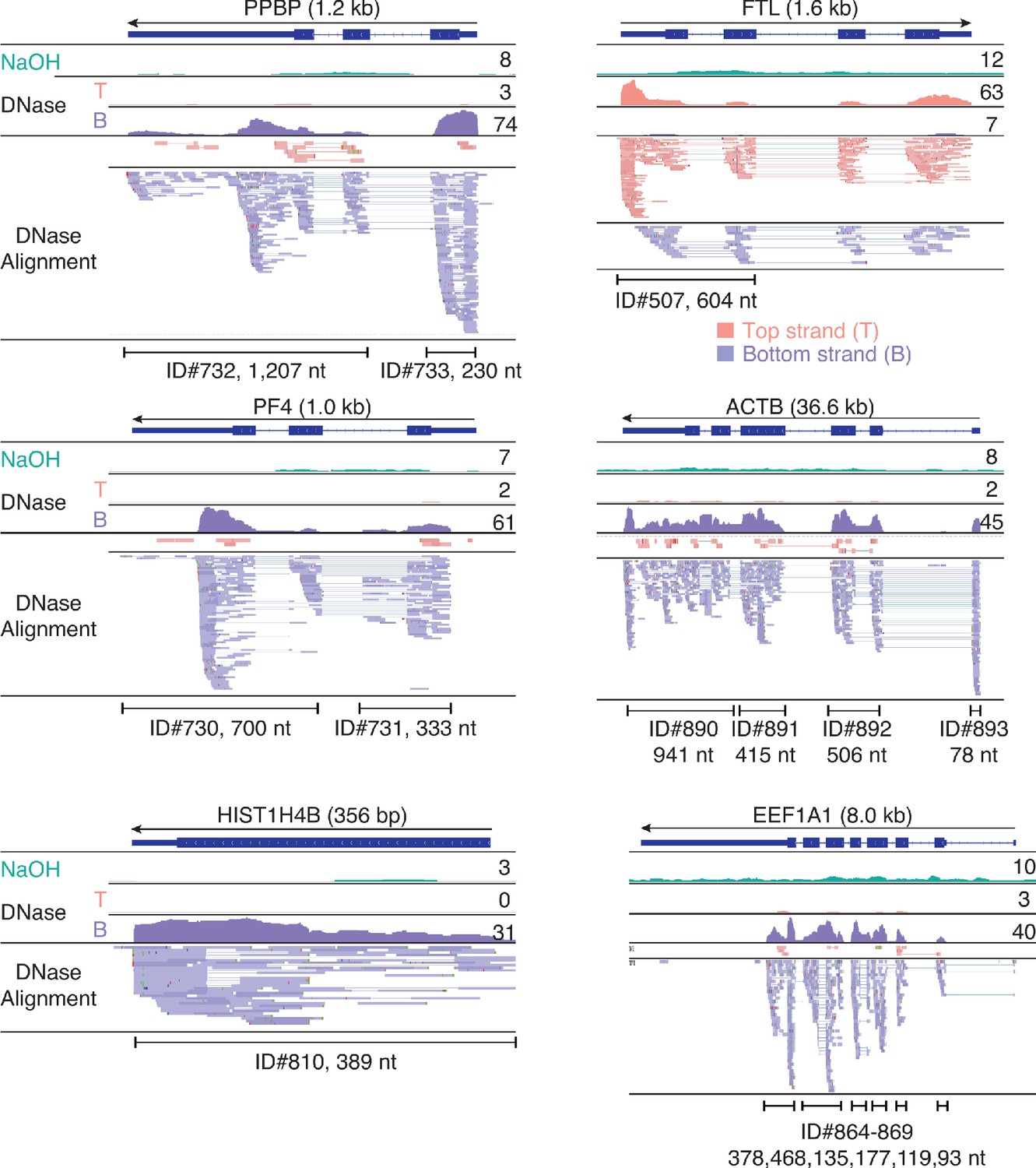
IGV screenshots showing examples of peaks consisting of heterogenous RNA fragments extending across protein-coding gene exons.
Gene names are indicated at the top with the length of the gene indicated in parentheses and an arrow below indicating the 5’ to 3’ orientation of the encoded mRNA. IGV coverage plots and alignments are labeled as in Figure 7 with the peak called by MACS2 delineated by the bracketed line with the peak ID number and length indicated below. The antisense reads in the FTL gene (top right) are discussed further in Figure 13—figure supplement 1 below.
Figure 7—figure supplement 2
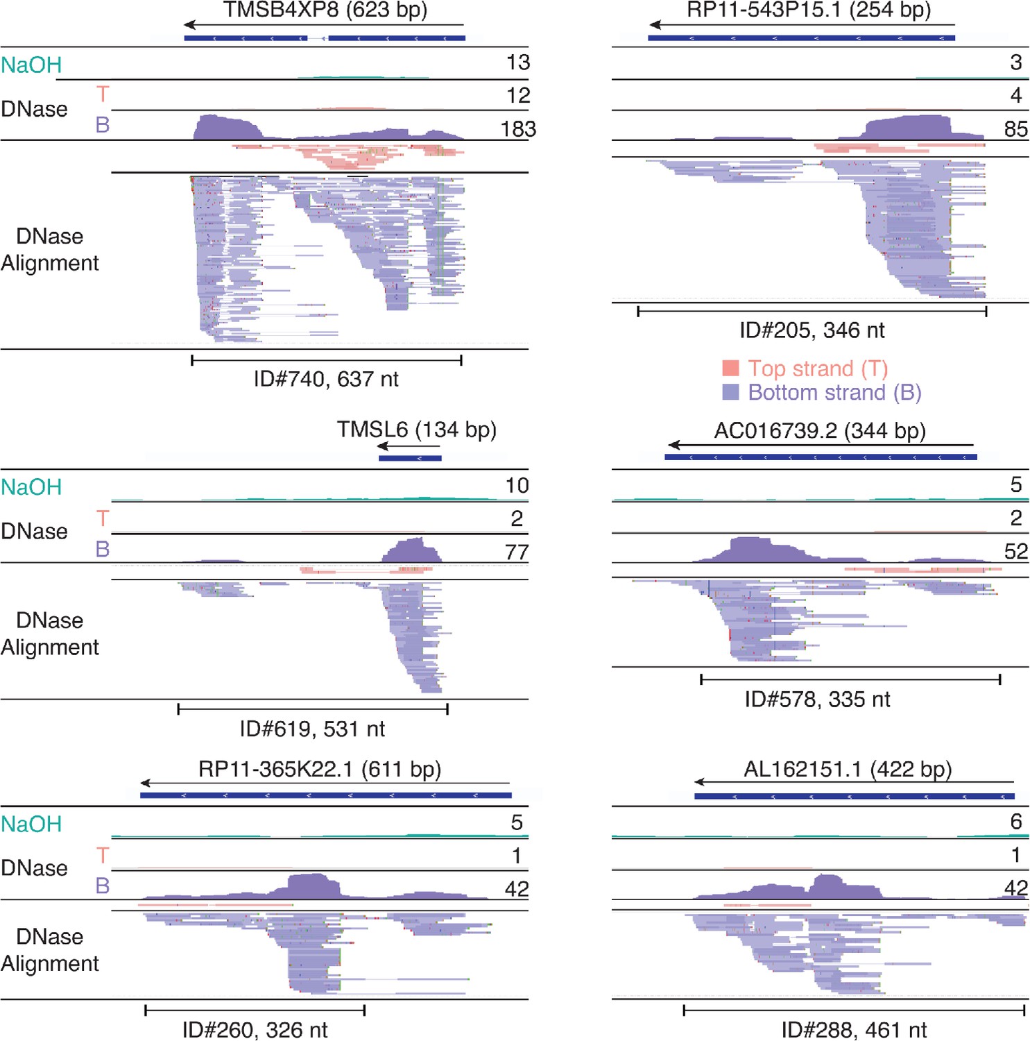
IGV screenshots showing examples of peaks consisting of heterogenous RNA fragments mapping to pseudogenes.
Pseudogene names are indicated at the top with the length of the pseudogene indicated in parentheses and an arrow indicating the 5’ to 3’ orientation of the encoded RNA. IGV coverage plots and alignments are labeled as in Figure 7 with the peak called by MACS2 delineated by the bracketed line with the peak ID number and length indicated below. When necessary, reads shown in alignment track were down sampled to maximum of 100 for display.
Figure 7—figure supplement 3
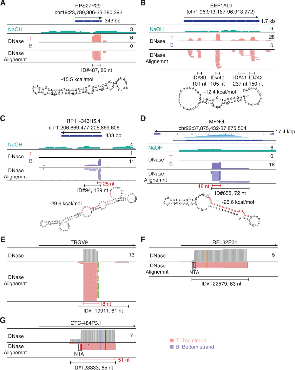
IGV screenshots showing example of peaks mapping to exons or pseudogenes that are comprised of or contain RNA fragments with discrete 5'- and 3'-ends (defined as > 50% of the deduplicated reads having identical 5' and 3' ends).
Gene names are indicated at the top with the hg19 coordinates of the called peak indicated in parentheses and the arrow below indicating the 5’ to 3’ orientation of the encoded RNA. IGV coverage plots and alignments are labeled as in Figure 7 with the peak called by MACS2 delineated by the bracketed black line with the peak ID number and length indicated below. (A, B) Peaks with discrete 5' and 3' ends that can be folded by RNAfold into secondary structures with ΔG ≤ −12 kcal/mol. In panel B, which shows a pseudogene with multiple called peaks, the predicted secondary structure is that of peak ID#40 (asterisk) for which >50% of the reads have discrete 5' and 3' ends. Other peaks in this category not shown in the Figure were ID#s T19005, T25471, and T38057 (Supplementary file 1). (C, D) Peaks that can be folded by RNAfold into secondary structures with ΔG ≤ −12 kcal/mol that contain segments (red) corresponding to separate shorter RNAs with discrete 5'- and 3'-ends that comprise part of the peak. The most stable predicted secondary structure and its MFE (ΔG) computed by RNAfold are shown below. Other peaks in this category not shown in the Figure were ID#s T3803*, T13916, T20238, T25941, T34313*, and T34462; the peaks marked with asterisks contain discrete short (14–15 nt) RNAs. (E–G) Peaks that cannot be folded by RNAfold into stable secondary structures but are comprised of or contain multiple reads with discrete 5' and 3' ends. NTA/black boxes are non-templated nucleotides added during TGIRT-seq library preparation.
Figure 8 with 1 supplement

Identification and characterization of repeat RNAs in human plasma.
(A) Density plot showing the range of peak lengths for different types of repeat sequences in the combined datasets for DNase-treated plasma RNA (n = 15). (B) Density plot showing the percentage of gene body covered by TGIRT-seq reads for all detected repeat RNAs. The normalized coverage of each repeat sequence in the combined plasma RNA datasets is plotted against the normalized size of the gene (100 bins). (C) Fitted beta distribution for the numbers of repeat sequences with different proportions of (+) orientation reads in combined datasets for NaOH-treated plasma DNA datasets (n = 4). The fitted beta distribution was used in an Empirical Bayes method to identify RNA repeats with significant differences in the percentage of (+) orientation reads in the combined plasma RNA datasets compared to the combined plasma DNA datasets, as described in Materials and methods. (D) Swarm plot showing the difference (Δ) between the percentage of (+) orientation reads in the combined plasma RNA datasets versus the combined plasma DNA datasets for different short tandem repeat element RNAs. The top ten tandem repeats with the highest (+) orientation enrichments in plasma RNA compared to plasma DNA datasets are named in the plot. (E) Volcano plot of fold difference in the normalized read count of transposable elements in DNase-treated plasma RNA (n = 15) compared to NaOH-treated plasma DNA (n = 4). The reads corresponding to repeat sequences in the initial mapping were remapped by SalmonTE to Repbase transposable elements, quantified, and compared to assess differences in the normalized read counts in the combined DNase-treated plasma RNA datasets versus the combined NaOH-treated plasma DNA datasets. Each point represents an annotated transposable element, with those in red having a fold-change with an adjusted p-value < 0.05. The top ten transposable elements with the highest fold changes and p-values < 0.05 are named in the plot.
Figure 8—figure supplement 1
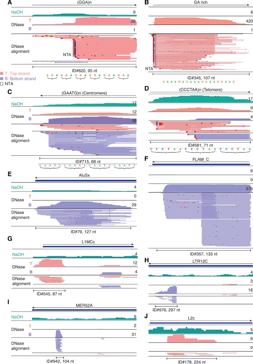
IGV screenshots showing examples of repeat and retrotransposable element RNAs detected in plasma by TGIRT-seq.
(A–D) Simple repeats, including centromeric and telomeric repeats. (E–J) Retrotransposable element RNAs. The repeat or transposable element RNA is named at the top with an arrow below indicating the 5' to 3' orientation of the RNA. The tracks below show coverage plots and read alignments for the peak region in combined datasets for NaOH-treated plasma DNA (n = 4; combined top and bottom strands (turquois)) or DNase-treated plasma RNA (n = 15; Top strand (T), pink and Bottom strand (B), purple) based on the number of deduplicated reads indicated to the right. Colors other than pink or purple in the read alignments indicate bases that do not match the reference sequence (red, green, blue, and brown indicate thymidine, adenosine, cytidine, and guanosine, respectively). The peak called by MACS2 is delineated by a bracketed line below the alignments with the peak ID and length indicated below. Close ups of simple repeat sequences (not to scale) are shown below the peak ID. AluSx, Alu subfamily Sx; FLAM_C, free left Alu monomer subfamily C; L1MCc, mammalian-wide LINE-1 (L1M) family Cc; LTR12C, LTR element 12C; MER52A, medium reiteration frequency interspersed repeat LTR from ERV1 endogenous retrovirus; L2c, LINE-2 family c; NTA/black boxes are non-templated nucleotides added during TGIRT-seq library preparation.
Figure 9
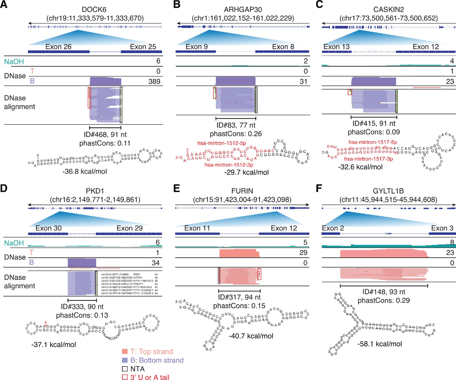
IGV screenshots showing examples of peaks corresponding to putatively structured, full-length excised intron RNAs detected in plasma by TGIRT-seq peak calling.
(A–C) Full-length excised intron RNAs that correspond to annotated agotrons or mirtrons. (D–F) Full-length excised intron RNAs that do not correspond to annotated agotrons or mirtrons. Gene names are indicated at the top with the hg19 coordinates of the called peak in parentheses and an arrow below indicating the 5’ to 3’ orientation of the encoded RNA. The top track shows the gene map (exons, thick bars; intron, thin lines), with the relevant part of the gene map expanded below. The tracks below the gene map show coverage plots and read alignments for the peak region in combined datasets for NaOH-treated plasma DNA (n = 4; combined top and bottom strands, turquoise) or DNase-treated plasma RNA (n = 15; Top strand (T), pink and Bottom strand (B), purple) based on the number of deduplicated reads indicated at the right in the coverage tracks. Colors other than pink or purple in the read alignments indicate bases that do not match the reference sequence (red, green, blue, and brown indicate thymidine, adenosine, cytidine, and guanosine, respectively). The peak called by MACS2 is delineated by a bracketed line with the peak ID, length, and phastCons score for 46 vertebrates including humans indicated below (see phylogenetic tree in Figure 10). The most stable predicted secondary structure and its MFE (ΔG) computed by RNAfold are shown below the peak ID. The annotated mature miRNA and passenger strands of mirtrons are highlighted in red within the predicted secondary structure. Red boxes, short (1–2 nt) non-templated 3' U or A tails; NTA/black boxes are non-templated nucleotides added by TGIRT-III to the 3' end of cDNAs (5' end of the RNA sequence) during TGIRT-seq library preparation.
Figure 10

Bar graphs showing phastCons scores for 44 full-length excised introns detected in human plasma.
PhastCons scores were calculated for 10 primates, 33 placental mammals, and 46 vertebrates shown in the phylogenetic tree on the right. PhastCons calculates the probability that a nucleotide belongs to a conserved sequence with the score for the peak calculated by averaging the score for each nucleotide within the peak. Scores can range from 0 to 1, with 1 being the most conserved, and 0 being the least conserved. The red line indicates a phastCons score of 0.5. M1-7 are full-length excised intron RNAs that encode non-high confidence miRNA: M1, mir-1225; M2, mir-4721; M3, mir-7108; M4, AC068946.1; M5, mir-6821; M6, mir-6891; M7, mir-1236.
Figure 11 with 1 supplement
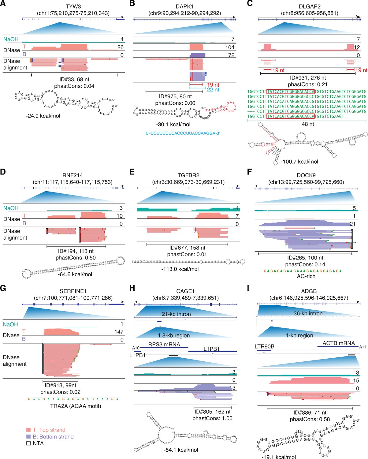
IGV screenshots showing examples of peaks mapping within introns.
Gene names are indicated at the top with the hg19 coordinates of the called peak in parentheses and an arrow below indicating the 5’ to 3’ orientation of the encoded RNA. IGV screenshots are labeled as in Figure 9. (A–E) Peaks corresponding to intron RNA fragments that can be folded into stable stem-loop structures. The predicted stem-loop structure for the peak in panel B includes a 19-nt segment (red), which corresponds to a separate 19-nt RNA that is a major component of the called peak and was accompanied by a separate 22-nt antisense RNA (blue) that is complementary to the 19-nt RNA. The predicted stem-loop structure in panel C is comprised of imperfect tandem repeats of a 48-nt sequence (green), part of which (red) corresponds to a separate 19-nt RNA that maps with fewest mismatches to the two terminal repeat units. The peaks in panels D and E are comprised of two complementary segments of long inverted repeats (46 bp with no mismatches and 65 bp with one mismatch, respectively), with the peak in panel E corresponding to an annotated binding site for double-stranded RNA-binding protein ILF3. (F, G) Peaks corresponding to intron RNA fragments that are not predicted by RNAfold to fold into stable secondary structures. (H, I). Peaks corresponding to short, putatively structured segments of mRNAs that had retrotransposed into long introns. The top track shows the gene map with the long intron to which the peaks mapped expanded below. The small blue line delineates the retrotransposed mRNA sequences with a short poly(A) tail and proximate LINE-1 elements expanded below. The small black bar delineates the region containing the called peak that is expanded in the IGV plots below. The most stable predicted secondary structure and its MFE (ΔG) computed by RNAfold are shown below the peak ID. When necessary, reads shown in alignment tracks were down sampled to a maximum of 100 for display. NTA/black boxes are non-templated nucleotides added during TGIRT-seq library construction.
Figure 11—figure supplement 1
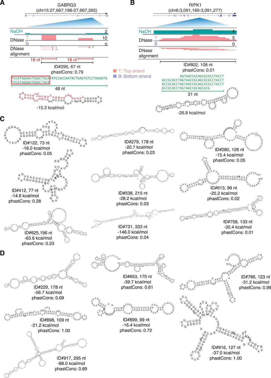
IGV screenshots and predicted secondary structures for peaks corresponding to intron RNA fragments.
(A, B) Intron peaks comprised of complex tandem repeats. The predicted stem-loop structure for the peak in panel A includes two 19-nt segments that correspond a 19-nt RNA (red) with reads distributed between the two segments. (C) Most stable RNA secondary structures predicted by RNAfold for peaks corresponding to intron RNA fragments. (D) Most stable RNA secondary structures predicted by RNAfold for peaks mapping to retrotransposed mRNA sequences within long introns. In panels C and D, the length of the peak is indicated next to the peak ID, and the most stable predicted secondary structure and its MFE (ΔG) computed by RNAfold are shown below.
Figure 12 with 1 supplement
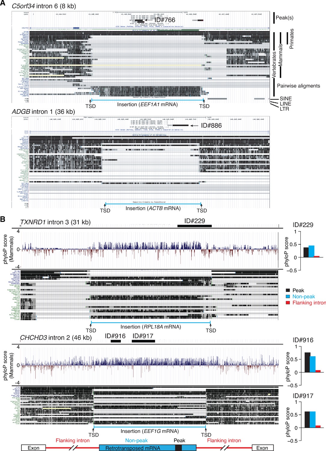
Genome browser (UCSC) screenshots showing examples of long introns containing retrotransposed mRNAs sequences that are called as peaks and sequence conservation across such introns.
(A) Two examples of long introns containing retrotransposed mRNA sequences that are called as peaks. The host gene, intron number, and intron length are indicated at the top, with the called peak or peaks (thick black line(s)) and peak ID indicated in the top track. The tracks below show alignments of genomic sequences of different organisms. Taxonomic ranks are shown at the top right, and the complete phylogenetic tree for the aligned sequences is shown in (Figure 12—figure supplement 1). The locations of nearby SINE, LINE, and LTR-containing retroelements in the human genome are shown below the alignments. The inserted retrotransposed mRNA sequence (bracketed blue line at the bottom) is identified by gap in genomic sequence for organisms that do not contain the insertion and by target site duplications (TSDs; 5–20 nt direct repeats) flanking the inserted sequence. Additional examples of long introns containing retrotransposed mRNA sequences that are called as peaks are shown in Figure 12—figure supplement 1. (B) Sequence conservation as measured by phyloP scores across long introns containing retrotransposed mRNAs sequences that are called as peaks. The gene name, intron number, and length of the intron are indicated at the top, with the position of the called peak delineated by a thick black line. The track below shows phyloP scores for placental mammals based on the pairwise alignment of genomic sequences from the different organisms in the genome browser alignments below. The inserted retrotransposed mRNA sequence (bracketed blue line at bottom) is identified by a gap in the genomic sequence for organisms that do not contain the insertion and by target site duplications (TSDs, 5–20 nt direct repeats) flanking the inserted sequence. The bar graphs to the right of the phyloP tracks show average phyloP scores for the called peak, flanking regions of the retrotransposed mRNA sequence, and 5'- and 3'-flanking regions of the host intron (see schematic at bottom). PhyloP scores are -log10 (p values) for the difference between the measured evolutionary conservation at a position in an alignment relative to that expected for a null hypothesis of neutral evolution. The score for each region was calculated by averaging the scores for each position in that region. Positive and negative scores indicate slower and faster evolution rates than expected from a neutral evolution model calculated from the phylogenetic tree (Ramani et al., 2018).
Figure 12—figure supplement 1
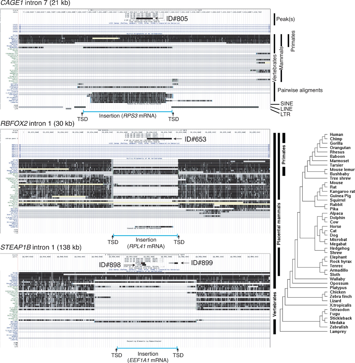
Genome browser (UCSC) screenshots showing additional examples of long introns containing retrotransposed mRNAs sequences that are called as peaks.
The host gene, intron number, and intron length are indicated at the top, with the called peak or peaks (thick black line(s)) and peak ID indicated in the top track. The customized tracks below show alignments of genomic sequences of different organisms (phylogenetic tree shown to the right), and locations of nearby SINE and LINE elements shown below. The inserted retrotransposed mRNA sequence (bracketed blue line at the bottom) is identified by gap in genomic sequence for organisms that do not contain the insertion and by target site duplications (TSDs; 5–20 nt direct repeats) flanking the inserted sequence.
Figure 13 with 2 supplements
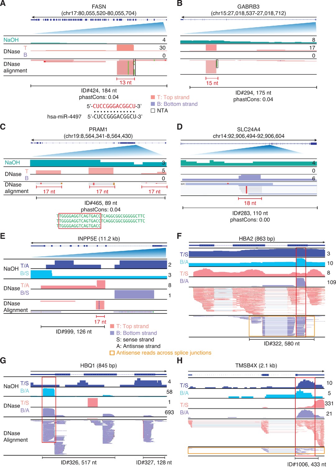
IGV screenshots showing examples of peaks corresponding to antisense RNAs detected in plasma by TGIRT-seq peak calling.
Gene names are indicated at the top with the hg19 coordinates of the called peak indicated in parentheses and an arrow below indicating the 5’ to 3’ orientation of the encoded mRNA. (A–D) Antisense peaks that map within introns and correspond to or contain short RNAs with discrete 5' and/or 3' ends (red). The IGV screenshots in these panels are labeled as in Figure 9. The 13-nt RNA in panel A corresponds to part of miR-4497 (alignment shown below). (E–H) Antisense peaks mapping to genes that are highly represented in plasma. In these panels, separate coverage plots are shown for the top (T) and bottom (B) strands for the NaOH-treated plasma DNA samples, and top and bottom strands are additionally labeled as sense (S) or antisense (A) depending upon the 5' to 3' orientation of the mRNA encoded by the gene displayed in IGV. The red boxes extending vertically across the read alignments and coverage plots delineate RNA peaks that are mirrored by DNA peaks in NaOH-treated plasma DNA, and the horizontal orange boxes delineate antisense reads that extend across multiple spliced exons. When necessary, reads shown in alignment tracks were down sampled to maximum of 100 for display.
Figure 13—figure supplement 1
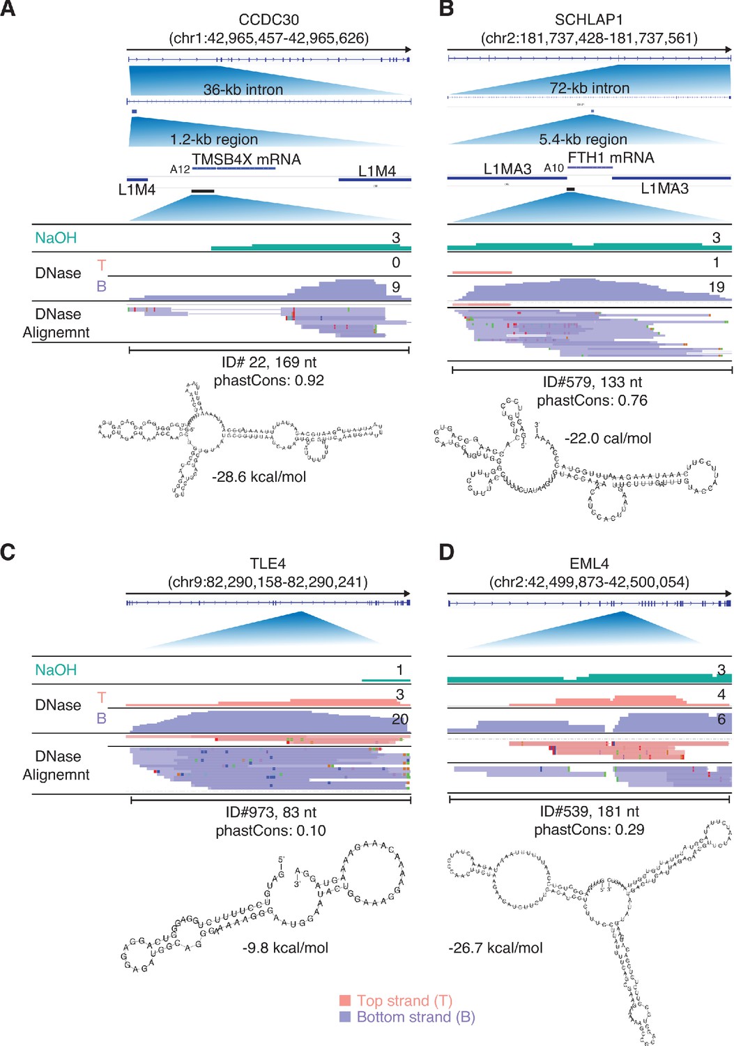
IGV screenshots showing additional examples of peaks mapping to the antisense strand of introns in protein-coding genes.
Gene names are indicated at the top with the hg19 coordinates of the called peak indicated in parentheses and an arrow below indicating the 5’ to 3’ orientation of the encoded mRNA. IGV coverage plots and alignments are labeled as in Figure 9 with the peak called by MACS2 delineated by a bracketed black line with the peak ID number, length, and phastCons score calculated for 46 vertebrates below. The most stable predicted secondary structure and its MFE (ΔG) computed by RNAfold are shown below. (A, B) Two antisense peaks corresponding to retrotransposed segments of mRNAs. The top shows the gene map with the long (36 and 72 kb) introns to which the peaks mapped expanded below. The small blue bar below the intron delineates the retrotransposed mRNA segment with a short poly(A) tail and proximate LINE-1 elements expanded below. The black line below the retrotransposed mRNA segment delineates the MACS2 RNA peak region, which is further expanded in the IGV screen shots below. (C, D) Two other antisense intron peaks and their predicted secondary structures.
Figure 13—figure supplement 2
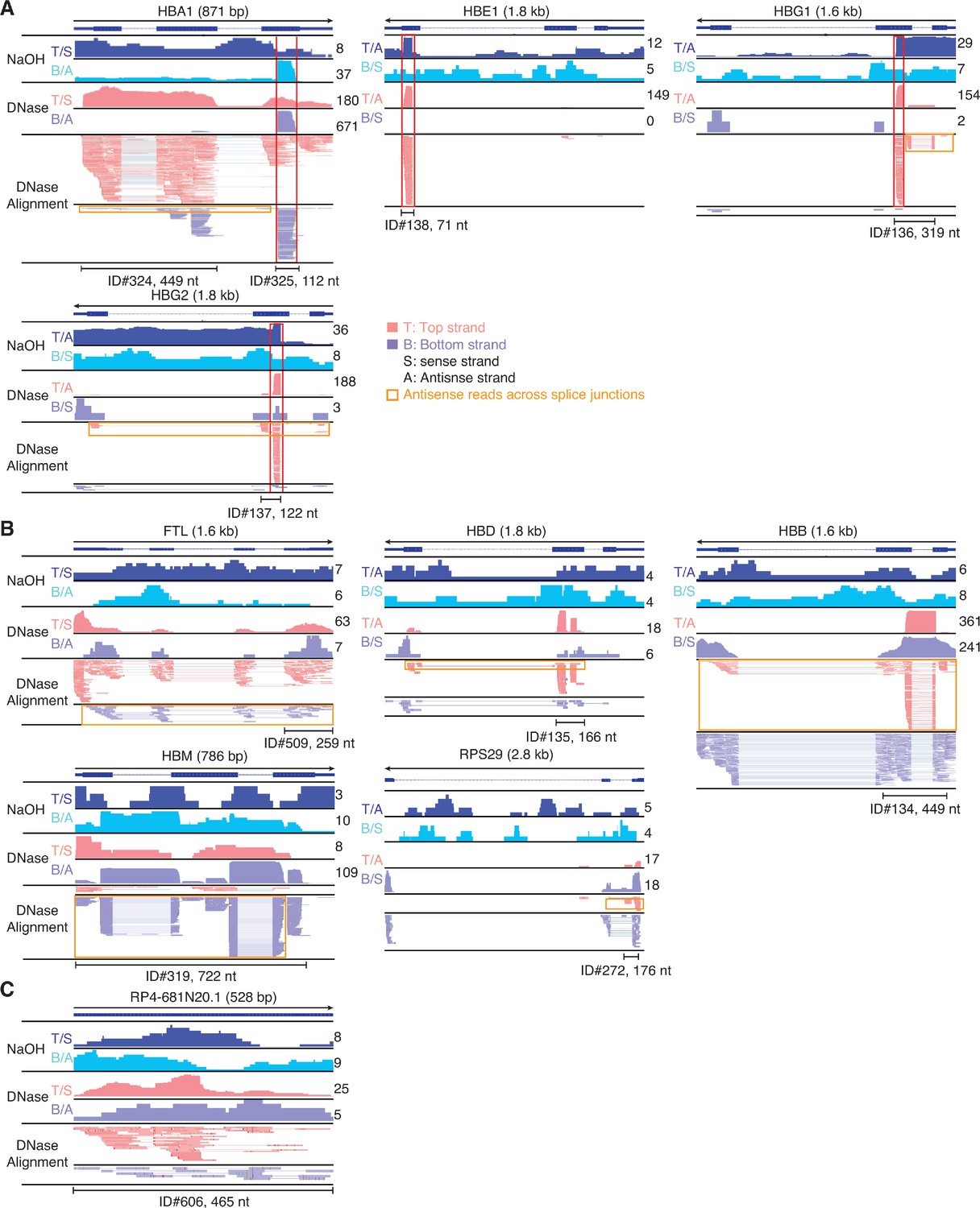
IGV screenshots of other peaks mapping to the antisense strand of annotated genes or pseudogenes.
Gene names are indicated at the top with the length of the gene indicated in parentheses and an arrow below indicating the 5’ to 3’ orientation of the mRNA or annotated pseudogene transcript. IGV screenshots are labeled as in Figure 9, but with separate coverage plots shown for the top (T) and bottom (B) strands for the NaOH-treated plasma DNA samples, and the top and bottom strands indicated as sense (S) or antisense (A) depending on the orientation of the mRNA or annotated pseudogene transcript. The RNA peak is delineated by a bracketed black line, with the peak ID number and length indicated below. Reads shown in the alignment tracks were down sampled to a maximum of 100. (A) Antisense peaks (other than the three shown in Figure 13F–H) that map to genes that are highly represented in plasma and contain regions mirrored by DNA peaks in NaOH-treated plasma DNA sample red boxes extending vertically across the alignments and coverage plots. (B) Other antisense peaks that map to mRNAs that are highly represented in plasma. (C) An antisense peak that maps to a pseudogene. Horizontal orange boxes delineate antisense reads that extend across multiple spliced exons.
Author response image 1
Correlation matrix of protein coding genes detected in DNase I-treated pooled plasma RNA using the improved TGIRT-seq method in this work (n=12), previously by TGIRT-seq in DNase I-treated plasma RNA from a healthy male individual (n=3; SRP064378, datasets 12-14) (Qin et al., 2016), and healthy plasmas samples similarly prepared from five healthy females in a collaborative study with Dr. Naoto Ueno, M.D. Anderson.
For comparisons, CPMs for each gene in a dataset were normalized to the total number of mapped reads in that dataset, log2 transformed, and plotted. Spearman correlation coefficients are shown on the upper triangle. Numbers on the x and y axes of scatter plots are log2 transformed CPMs.
Tables
Key resources table
| Reagent type (species) or resource | Designation | Source or reference | Identifiers | Additional information |
|---|---|---|---|---|
| Biological sample (Homo sapiens) | Plasma | Innovative Research | IPLA-N-K2E | Human plasma pooled from healthy individuals |
| Commercial assay or kit | QIAamp ccfDNA/RNA kit | Qiagen | Qiagen 55184 | |
| Commercial assay or kit | SMART-Seq v4 Ultra Low Input RNA kit | Takara Bio | R400752 | |
| Commercial assay or kit | TGIRT-III reverse transcriptase | InGex, LLC | TGIRT |
Additional files
-
Supplementary file 1
Comprehensive peak annotations and supporting data.
- https://cdn.elifesciences.org/articles/60743/elife-60743-supp1-v3.xlsx
-
Transparent reporting form
- https://cdn.elifesciences.org/articles/60743/elife-60743-transrepform-v3.pdf
Download links
A two-part list of links to download the article, or parts of the article, in various formats.
Downloads (link to download the article as PDF)
Open citations (links to open the citations from this article in various online reference manager services)
Cite this article (links to download the citations from this article in formats compatible with various reference manager tools)
Identification of protein-protected mRNA fragments and structured excised intron RNAs in human plasma by TGIRT-seq peak calling
eLife 9:e60743.
https://doi.org/10.7554/eLife.60743


