Achieving functional neuronal dendrite structure through sequential stochastic growth and retraction
- Frankfurt Institute for Advanced Studies, Germany
- Ernst Strüngmann Institute (ESI) for Neuroscience in cooperation with Max Planck Society, Germany
- Center for Neurodegenerative Diseases (DZNE), Germany
- Department of Zoology, University of Cambridge, United Kingdom
- Max Planck Institute for Dynamics and Self Organization, Germany
- Faculty of Medicine, ICAR3R – Interdisciplinary Centre for 3Rs in Animal Research, Justus Liebig University Giessen, Germany
- Neuroscience Center, Institute of Clinical Neuroanatomy, Goethe University, Germany
- LIMES Institute, University of Bonn, Germany
Figures
Figure 1

Distinct stages of c1vpda dendrite differentiation during embryonic and larval stages.
(A) Imaging procedure throughout embryonic (E) stages. The eggs were imaged at higher temporal resolution in a time window ranging from 16−24 hrs AEL. Sketch (top row left) illustrating the experimental conditions, drawing (top row right) depicting the ordering of c1vpda branches (black: MB order 1, blue: lateral branch order 2, orange: lateral branch order > 2). Timeline and maximum intensity projections (middle row) of image stacks as well as reconstructions (bottom row) of a given representative c1vpda dendrite. White arrows in images and corresponding black arrows on reconstructions indicate exemplary changes between the time points (see main text). (B) Subsequent imaging of Larval instar (L) 1, 2, 3 stages with similar arrangements as in A. Times shown are AEL (after egg laying).
Figure 2 with 1 supplement
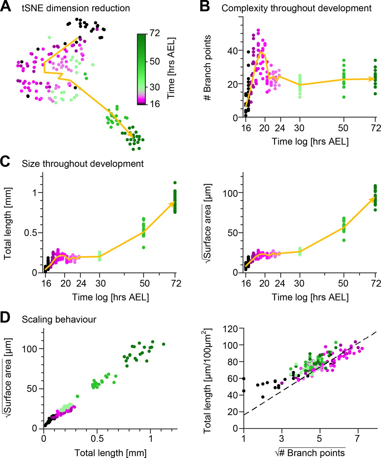
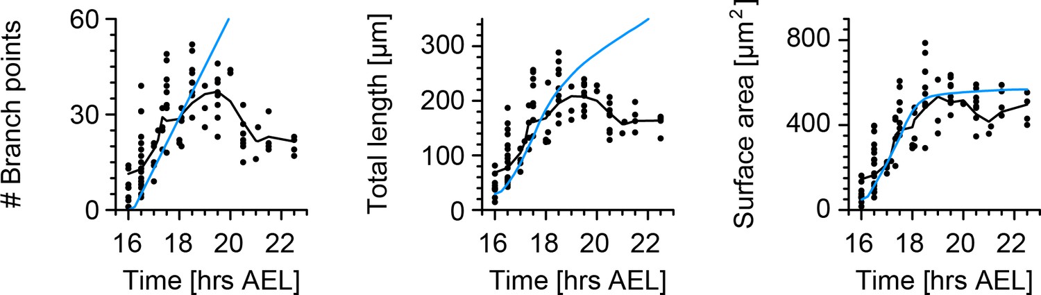
Quantification of c1vpda dendrite differentiation throughout development.
(A) A t-distributed stochastic neighbour embedding (tSNE) plot showing the entire dataset of neuronal reconstructions using a 49—dimensional morphometric characterisation reduced to two dimensions. (B) Time course of the number of branch points during development (see also Figure 6C). (C) Time courses of the total length of dendrite cable (left) and square root of the surface area (right) during development (see also Figure 6C). (D) Scaling behaviour of the square root of the surface area against total length (left) and total length against number of branch points (right) showing the relationships expected from the optimal wire equations (Cuntz et al., 2012; Baltruschat et al., 2020). The dashed line shows the average scaling behaviour of simulated synthetic trees ( simulations; see Materials and methods). In all panels, each dot represents one reconstruction with the colour scheme indicating imaging time AEL roughly dissecting embryonic (magenta) and larval (green) developmental stages (colour bar in A). The thick yellow arrows show trajectories averaging values of all reconstructions across two hour bins in A, and 1 hr bins in B and C for higher resolution. Data from reconstructions, neurons, animals. See also Figure 2—figure supplement 1 for details on the scaling in the different stages of development.
Figure 2—figure supplement 1
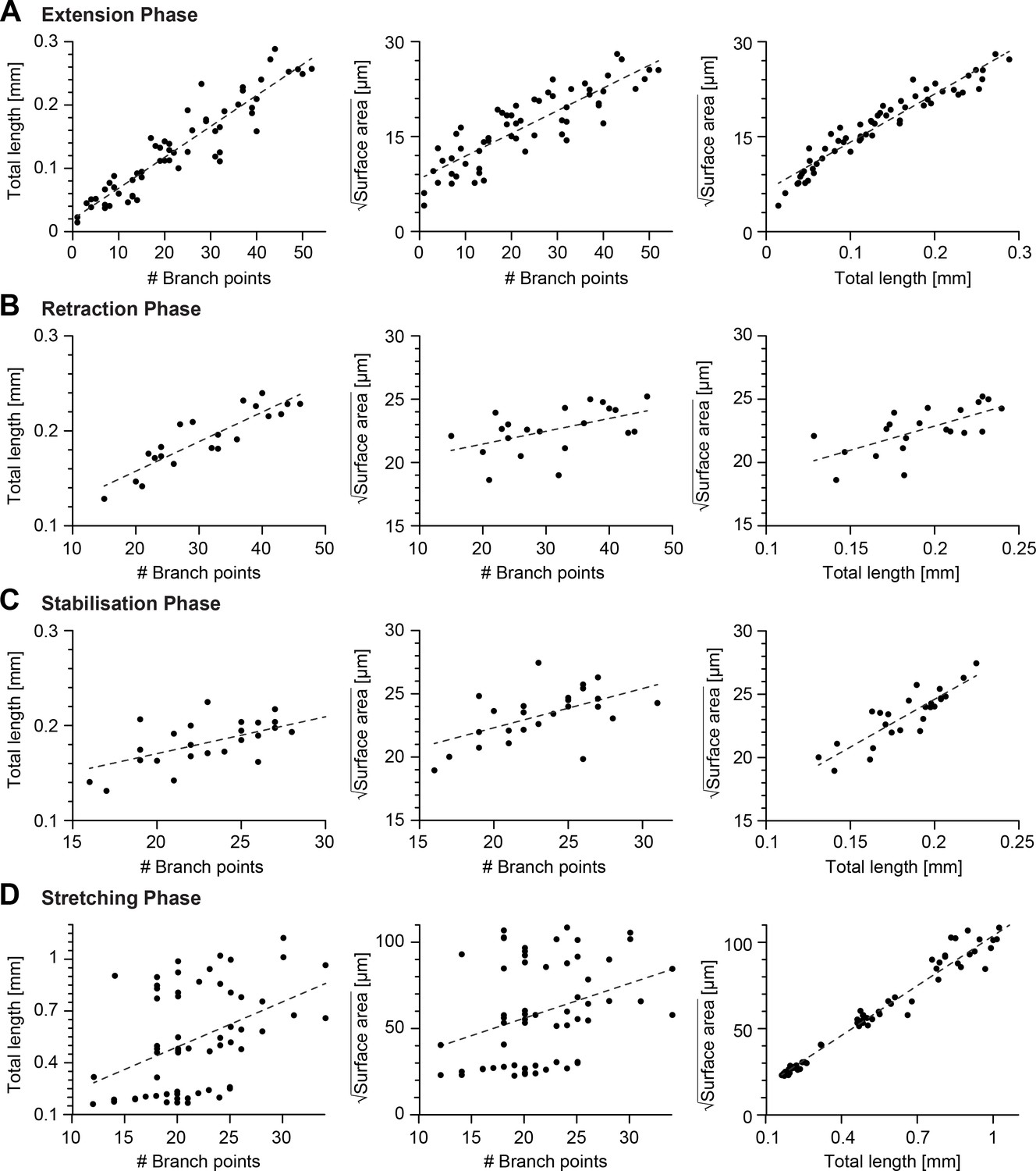
Scaling relations between key morphometrics during development.
(A–D) Linear fits of the number of branch points vs total cable length, number of branch points vs the square root of the dendrite surface area (middle) and total cable length vs the square root of the dendrite surface area (right) during the extension phase (16−18.5 hrs AEL, , from left to right , , ), retraction phase (18.5−20.6 hrs AEL, , from left to right , , ), stabilisation phase (20.6−24 hrs AEL, , from left to right , , ), scaling phase (24−72 hrs AEL, , from left to right , , ). In all panels, each black dot represents one reconstruction (overall ) black-dashed lines represent the best-fit.
Figure 3 with 1 supplement
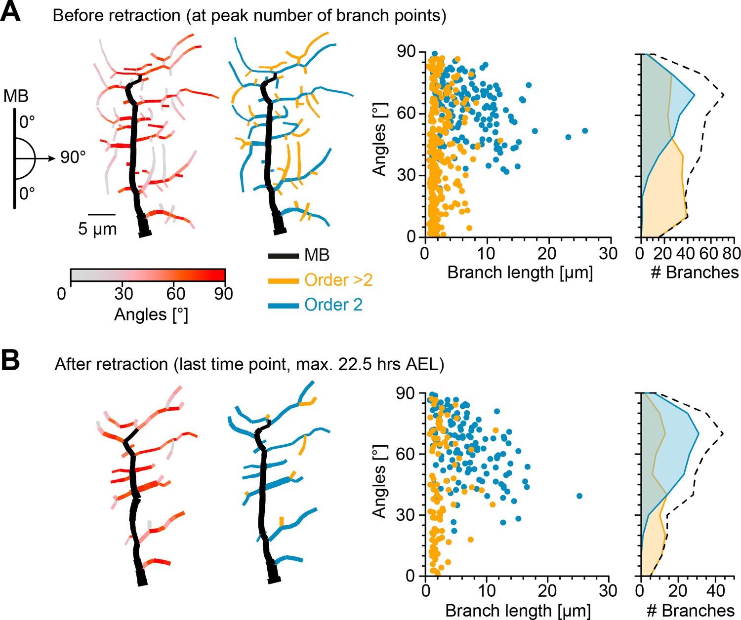
Retraction phase preferentially targets smaller, low orientation angle, higher-order lateral branches.
(A) Sketch illustrating lateral branch orientation angle and dendrite morphology of a sample c1vpda sensory neuron before retraction. Morphology on the left side is colour coded by branch segment angles and morphology on the right is colour coded by branch length order (MB is coloured in black; see Materials and methods). On the right, histograms for branch length (one dot per branch) and number of branches per angle are shown separated by branch length order (blue: order 2, orange: order > 2, branches). Dashed line represents the overall distribution of number of branches per angle. (B) Similar visualisation but for dendrites after retraction ( branches).
Figure 3—figure supplement 1
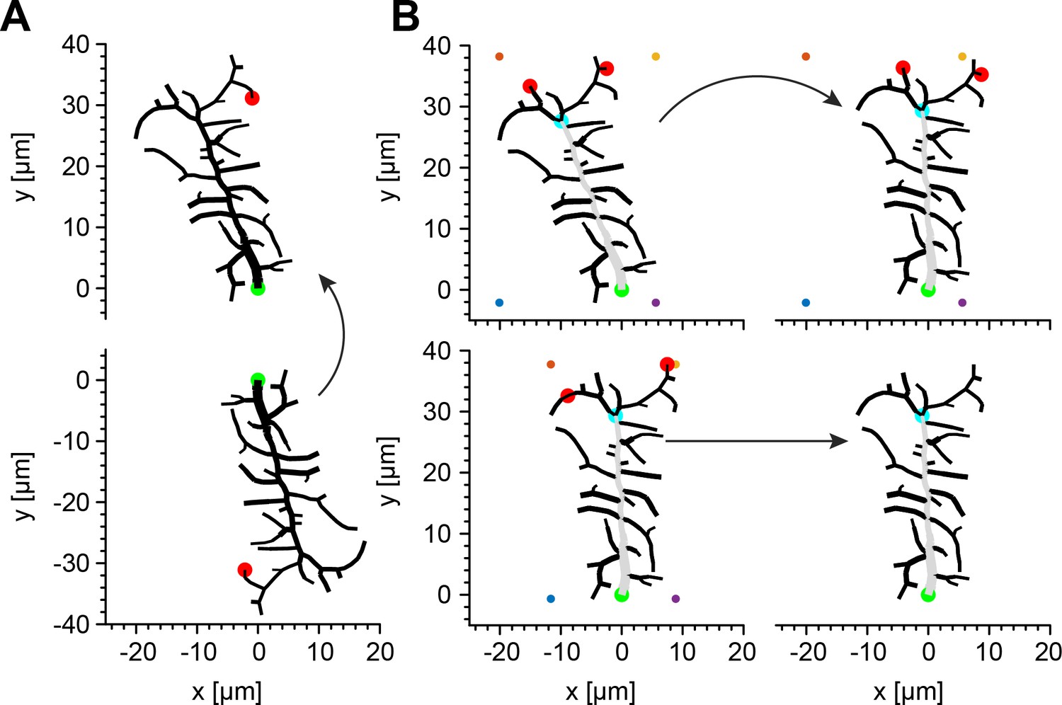
Illustration of the algorithm identifying the MB.
(A) As a first step, the algorithm translates the reconstruction of an arbitrary dendritic tree (bottom) by setting the root to x- and y-coordinates (0, 0) and rotates it until the terminal of the longest path of the tree (red circle) is set to x-coordinate (0) and the y-coordinate is set to a positive value. (B) At each new iteration in a subsequent refinement of the rotation, a bounding box (coloured dots) is generated around the dendritic tree and the closest node to the top left corner, and to the top right corner are found (red circles). The first common branch point in the paths of these nodes is defined as the provisional last node of the MB (light blue circle) and the tree is rotated until this node is set to x-coordinate (0). This procedure is repeated until the branch point of the MB in the current iteration is the same as the one in the previous iteration. In all panels, green circles represent the root of the dendritic tree and grey branches represent the MB.
Figure 4 with 5 supplements

Retraction increases branch bending curvature during larval contraction potentially facilitating signal transduction.
(A), (Top) Mean normalised Ca2+ responses of c1vpda dendrites during forward crawling. The signal was calculated as the fold change of the signal in the fluorescence ratio (see Materials and methods and Figure 4—figure supplement 1). signal amplitude was normalised for each trial. Data from six animals, neurons; solid pink line shows average values where data comes from neurons and dashed pink line where neurons. Standard error of the mean in pink shaded area. (Bottom) Average normalised contraction rate during crawling behaviour (similar plot as in top panel but in black colour). Segment contraction and Ca2+ responses were aligned to maximal segment contraction at . (B) (Top row) Simulated contraction of a c1vpda morphology by wrapping around a cylinder. (Main panel) Relationship between normalised curvature increase experienced by a single branch as a function of its orientation angle θ. (C) C1vpda dendrite morphologies before (left) and after (right) retraction. Morphologies are colour coded by local curvature increase during segment contraction. (D) Similar visualisation of the same data as in Figure 3 but for curvature increase before and after retraction. Dashed line represents the overall distribution of number of branches per curvature increase. Rightmost panel additionally shows the distribution (%) of retracted branches by bending curvature increase (red shaded area).
Figure 4—figure supplement 1
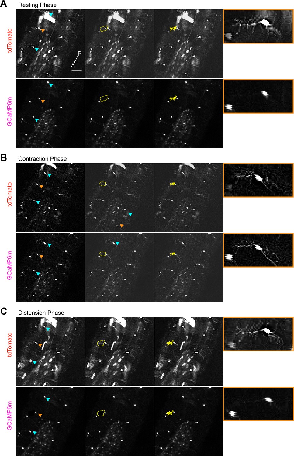
Calcium imaging of c1vpda dendrites during forward crawling.
(A) Representative images of c1vpda cells using a line that expresses CD4-tomato (top panels) and GCaMP6m (Bottom panels) in c1vpda neurons (w-; UAS-GCaMP6m; UAS-CD4-tdTomato, Gal4 2–21/MKRS), showing the ventral view of the larval body during resting phase. The GCaMP6m signal was extracted from cell indicated by the orange arrow (left Panels). Illustrative rough ROI’s (middle panels) used to generate the tight ROI’s around the cell dendrites (right panels). The rightmost insets with orange borders show zoomed in images of the neuron indicated by the orange arrow in the left panels. In B, images showing increased GCaMP6m activity in c1vpda dendrites during contraction, but in C, GCaMP6m activity decreased back to baseline during distension. Scale bar, 50 µm.
Figure 4—figure supplement 2

Tubular structure elliptical profile approximation.
(A) Representative sketch of tubular structures, with different orientation angles, deformation while being wrapped around a cylindrical surface. (B) Illustration of tubular structure with diameter 2r with orientation angle θ wrapped around a cylinder with radius R (top panel). Representative elliptical profile of a tubular structure wrapped around a cylinder. b and a represent the axes of the ellipse.
Figure 4—video 1
Video of c1vpda dendrites during forward crawling in real-time.
Same neurons as in Figure 4—figure supplement 1 (calcium channel GCaMP6m). Orange arrows indicate axis of contraction. Scale bar 50 µm.
Figure 4—video 2
Video of c1vpda dendrites during forward crawling in real-time.
Same neurons as in Figure 4—figure supplement 1 (calcium channel GCaMP6m). Orange arrows indicate axis of contraction. Scale bar 50 µm.
Figure 4—video 3
Video of c1vpda dendrites during forward crawling in real-time.
Same neurons as in Figure 4—figure supplement 1 (calcium channel GCaMP6m). Orange arrows indicate axis of contraction. Scale bar 50 µm.
Figure 5 with 1 supplement
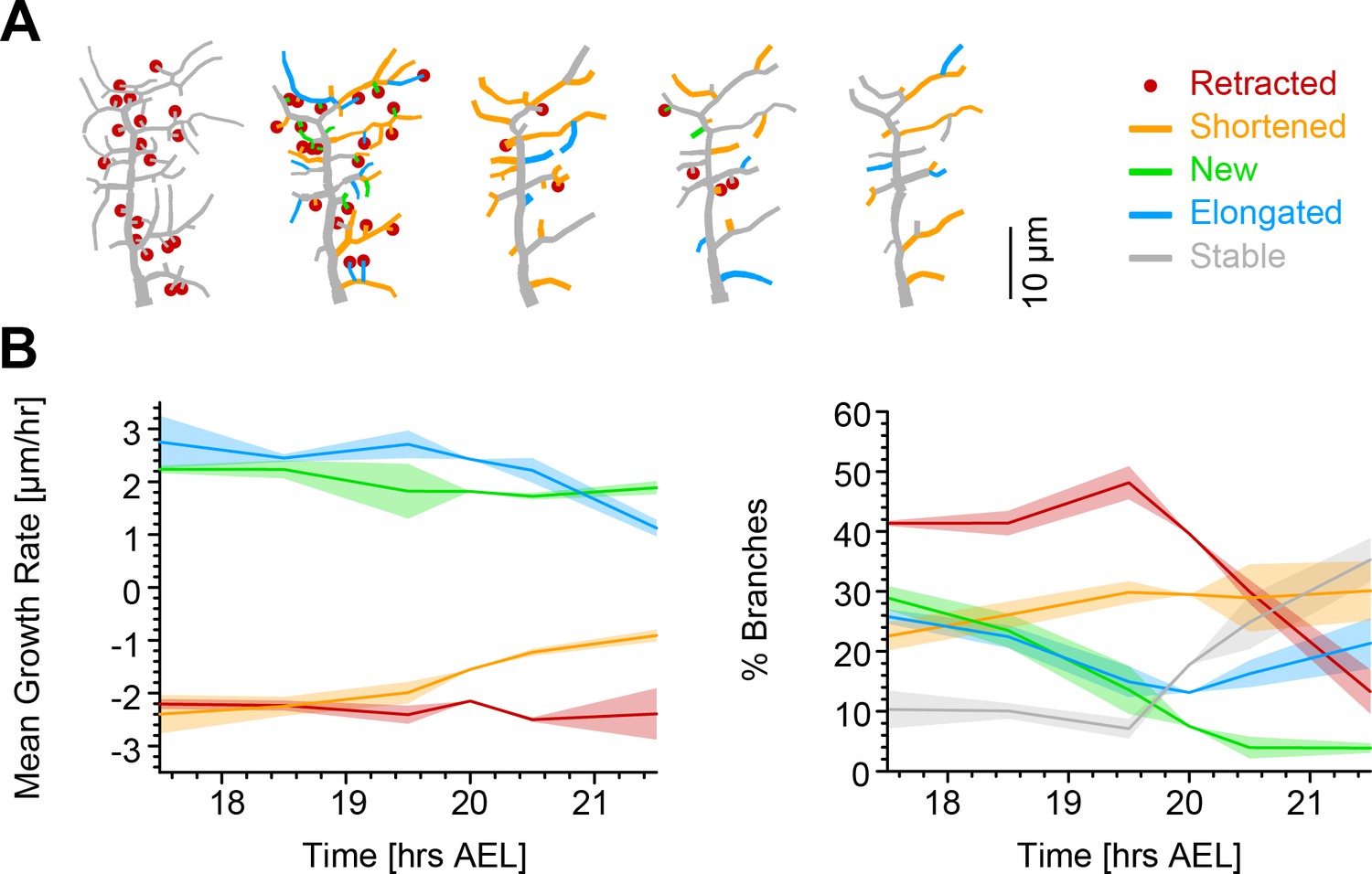
Single branch tracking analysis quantifies retraction phase dynamics.
(A) Dynamics of retraction phase for one sample c1vpda dendritic morphology with branches coloured by their respective dynamics, red circles–to be retracted; orange–shortened; green–newly formed; blue–elongating; grey–stable. (B) (Left) Branch dynamics similar to A but quantified as growth rates () for all branches of all dendrites tracked during the retraction phase, ; same colours as in A. (Right) Assignment of branches to the five types in A as a function of time. Shading represents the standard error of the mean.
Figure 5—figure supplement 1
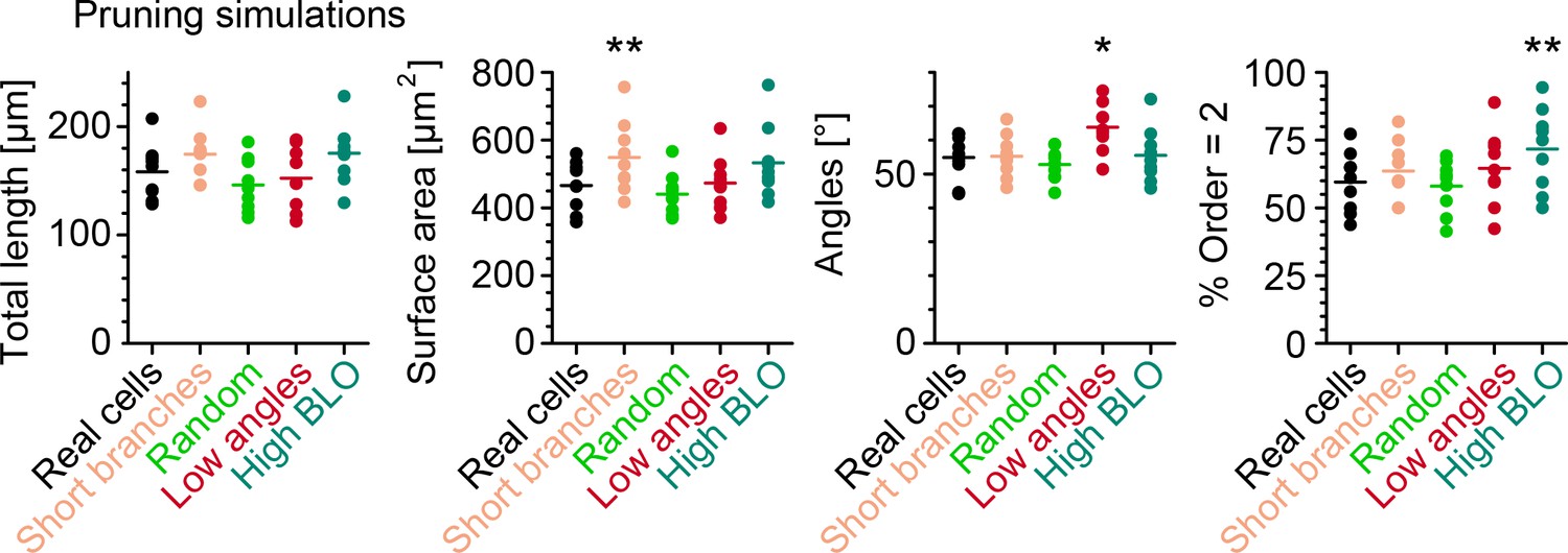
In silico simulations to quantify retraction phase dynamics.
Key morphometrics comparing real neurons after retraction with simulated retraction schemes applied on the morphology before retraction. Each dot is one morphology, bars indicate mean, and stars indicate p-values as follows: *, ** ( branches, neurons, from six animals).
Figure 6 with 1 supplement
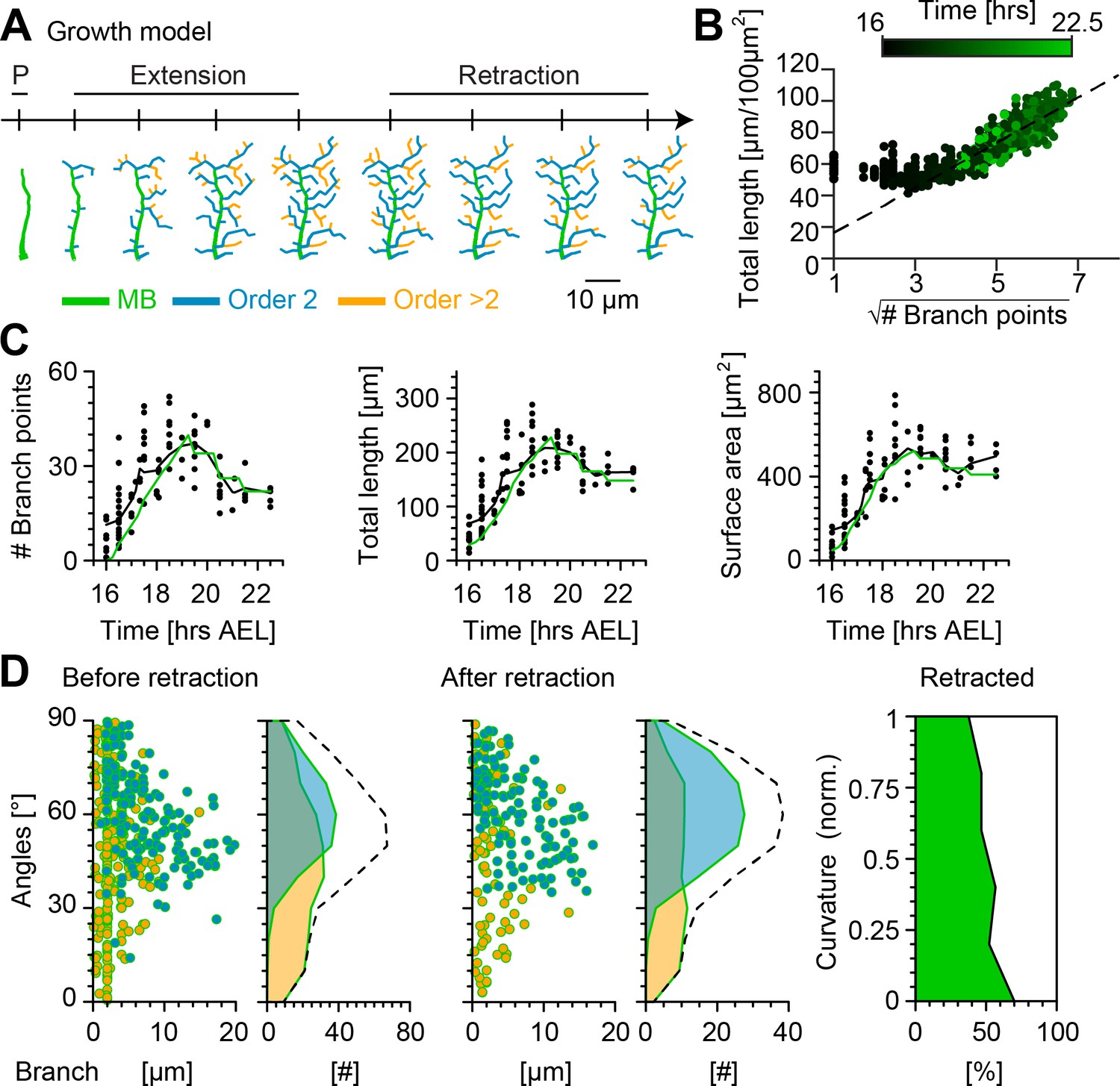
Computational growth model with stochastic retraction satisfies optimal wire constraints and replicates c1vpda dendrite growth.
(A) Synthetic dendrite morphologies of a sample c1vpda during the entire embryonic development ordered by their respective developmental stages: polarisation (P), extension and retraction, until the stabilisation phase. (B) Scaling behaviour of total length against the square root of branch points of the trees generated using the random retraction growth model. The dashed line shows the average scaling behaviour of the simulated MST trees used in Figure 2D ( simulations; ; see Materials and methods). (C) Time course of the number of branch points (), total length of dendrite cable () and surface area () during development until the stabilisation phase. In all panels, each black dot represents one reconstruction () black solid lines represent the moving average of the real neurons and green solid lines represent the mean behaviour of the synthetic trees (). (D) Representative visualisation of a random sample of synthetic trees before retraction (left, with same number of trees as in experimental data) histograms for branch length (one dot per branch) and number of branches per angle are shown separated by branch length order (Blue: order 2, Orange: order > 2). Dashed line represents the overall distribution of number of branches per angle. Similar visualisation (middle) of dendrites after retraction as well as summary histograms. Rightmost panel shows the distribution (%) of retracted branches by bending curvature increase (green shaded area).
Figure 6—figure supplement 1
Growth model without retraction does not replicate c1vpda dendrite growth.
Time course of the number of branch points (left), total length of dendrite cable (middle) and surface area (right) during embryonic development. Same arrangement and same data as in Figure 6B but for the growth model without retraction.
Appendix 1—figure 1
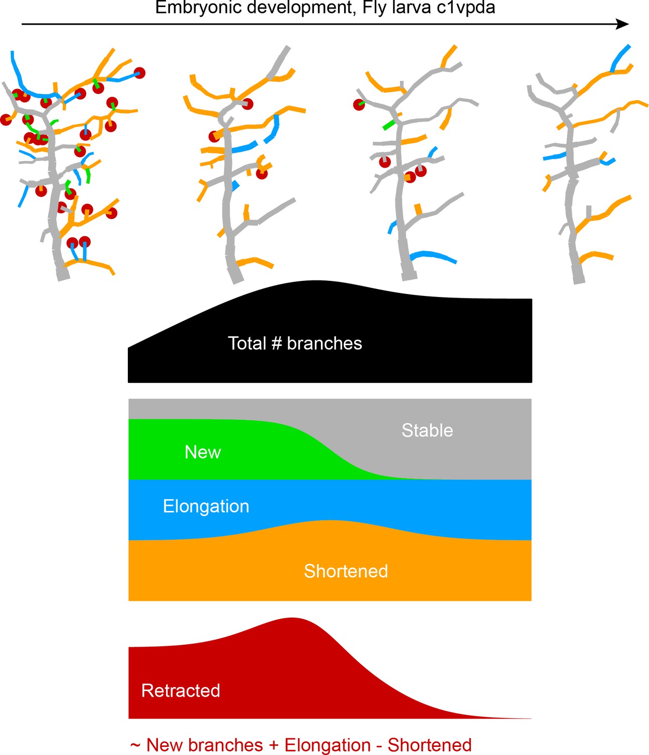
Sketch that illustrates visually the dynamics of branching during embryonic development of class I dendrites.
Tables
Key resources table
| Reagent type (species) or resource | Designation | Source or reference | Identifiers | Additional information |
|---|---|---|---|---|
| Genetic reagent (D. melanogaster) | 221 Gal4 | Ye et al., 2004 | ||
| Genetic reagent (D. melanogaster) | UAS-mCD8::GFP | RRID:BDSC_32187 | ||
| Genetic reagent (D. melanogaster) | UAS-IVS-GCaMP6m | RRID:BDSC_42748 | ||
| Genetic reagent (D. melanogaster) | UAS-CD4::tdTomato | RRID:BDSC_35837 | ||
| software, algorithm | Trees Toolbox (MATLAB) | Cuntz et al., 2010 | RRID:SCR_010457 (RRID:SCR_001622) | treestoolbox.org (mathworks.com) |
| software, algorithm | FIJI | Schindelin et al., 2012 | RRID:SCR_002285 | fiji.sc |
Additional files
Download links
A two-part list of links to download the article, or parts of the article, in various formats.
Downloads (link to download the article as PDF)
Open citations (links to open the citations from this article in various online reference manager services)
Cite this article (links to download the citations from this article in formats compatible with various reference manager tools)
Achieving functional neuronal dendrite structure through sequential stochastic growth and retraction
eLife 9:e60920.
https://doi.org/10.7554/eLife.60920


