Cell-scale biophysical determinants of cell competition in epithelia
- Department of Physics and Astronomy, University College London, United Kingdom
- London Centre for Nanotechnology, University College London, United Kingdom
- Department of Cell and Developmental Biology, University College London, United Kingdom
- Institute for Structural and Molecular Biology, University College London, United Kingdom
- Institute for the Physics of Living Systems, University College London, United Kingdom
- Department of Physics, Carnegie Mellon University, United States
Figures
Figure 1 with 5 supplements
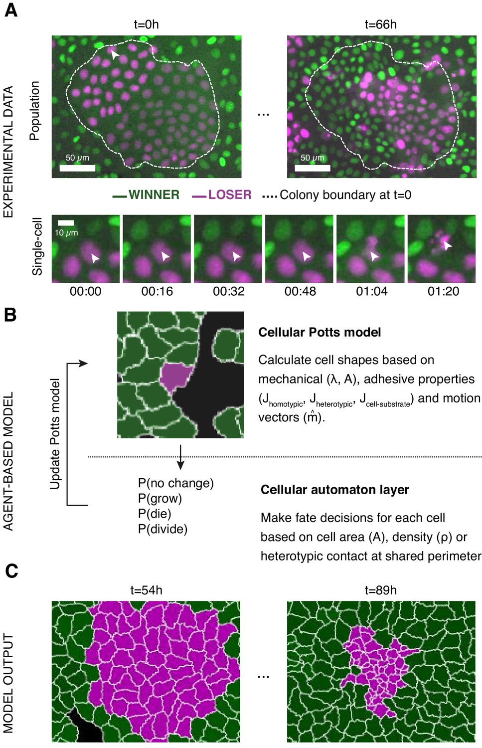
Experiments and simulations of cell competition.
(A) Experimental snapshots of competition between MDCKWT cells (winner, green) and MDCKScrib cells (loser, magenta) at the population scale (top) and the single-cell scale (bottom). Over the course of the experiment, the winner cells outcompete the loser cells whose area and number decreases (top) through apoptosis of individual cells (bottom). The arrowhead indicates the position of the dying cell examined in the bottom snapshots. The dashed line indicates the extent of the loser cell colony at the beginning of competition. (B) Framework of the multi-scale agent-based model used to simulate cell competition. The model consists of a Potts model and a cell automaton acting sequentially. The cellular Potts model first determines the cell shapes and position based on mechanical properties, such as intercellular adhesion and cell compressibility. Then a cell automaton decides whether cells grow, divide, or die based on a set of probabilistic rules that are algorithmically executed for each cell at each time point. These decisions are used to update the physical and geometrical properties of each cell before running the Potts model again. Further details about the cell behaviours included, the parameters, and the variables can be found in Figure 1—figure supplements 1 and 2. (C) The model outputs the time evolution of the organisation of the winner and loser cell types. These outputs can be quantitatively compared to experimental data.
Figure 1—figure supplement 1
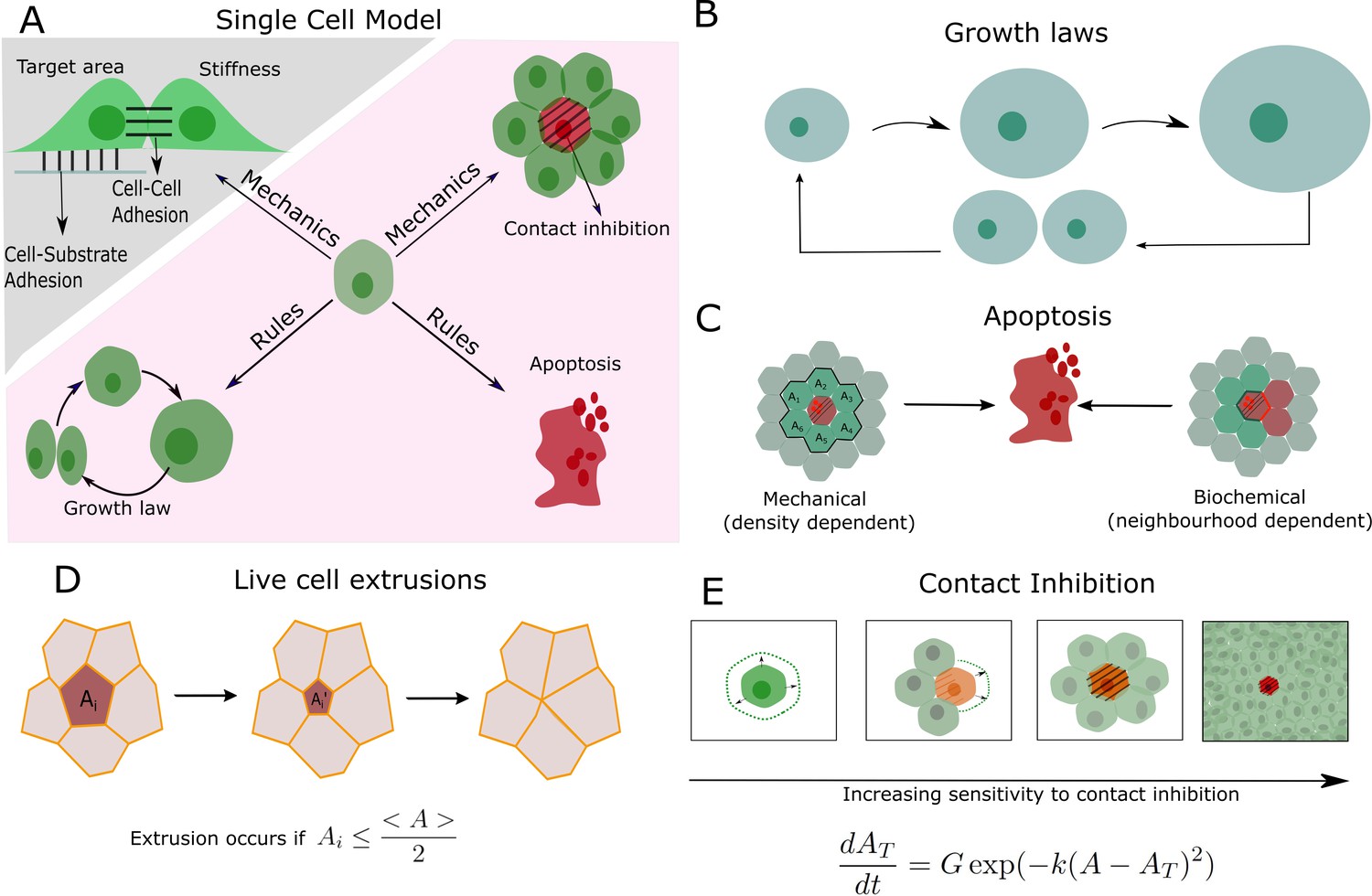
Physical and decision-making components of the multi-layered computational model.
(A) Schematic of the single-cell behaviours incorporated into the multi-scale agent-based model. A cellular Potts model is used to model physical interactions between cells, such as adhesion and compressibility (greyed region). An agent-based model (pink region) comprises cellular automaton rules describing cell growth, division, apoptosis, and contact inhibition. These rules are algorithmically executed for each cell at each time point. (B) Cells grow linearly in time and follow an adder mechanism for division control, in which a threshold size ΔAtot must be added before a cell can divide (Figure 1—figure supplement 3). (C) Two separate rules were implemented for apoptosis during mechanical competition (Figure 1—figure supplement 4A) and biochemical competition (Figure 1—figure supplement 5A). (D) Cells can also be removed from epithelia through live cell extrusion. Extrusion occurs if cell i’s area, Ai, decreases below half of the mean cell area of the population <A>, . (E) Schematic depiction of contact inhibition showing cell growth and movement are arrested when local cell density increases. The growth rate of a cell depends on how far its actual area A is from its target area AT.
Figure 1—figure supplement 2

Simulation workflow.
(A) Input variables are separated into three categories: physical parameters, cell automaton rules, and initial conditions. Physical parameters (grey) describe the cellular mechanical and physical properties, and these are calibrated using the experimental measurements given in the table. Cell automaton rules (pink) are run for each cell at each time point. They are parametrised using heuristic variables calibrated based on experimental data acquired on MDCK cells. Initial conditions describe the parameters needed to initialise the simulations. These replicate experimental conditions and are randomised with a chosen set of rules for each new simulation. (B) Multi-scale agent-based model consisting of a cellular Potts model coupled to a cellular automaton. The Potts model computes the mechanical equilibrium state of the system at each timestep based on the mechanical state of the cell and the values of cell parameters updated by the cellular automaton at the previous timestep. As input, it requires the initial conditions and the physical parameters of each cell. The cellular automaton model updates cellular parameters at each time point. As input at each timestep, it requires the conditions at the previous timestep computed by the Potts model and a table of heuristic rules. (C) The model outputs cell count, cell positions, cell size and shape, cell type, and cell fates for all time points. These outputs can be compared to experimental data.
Figure 1—figure supplement 3
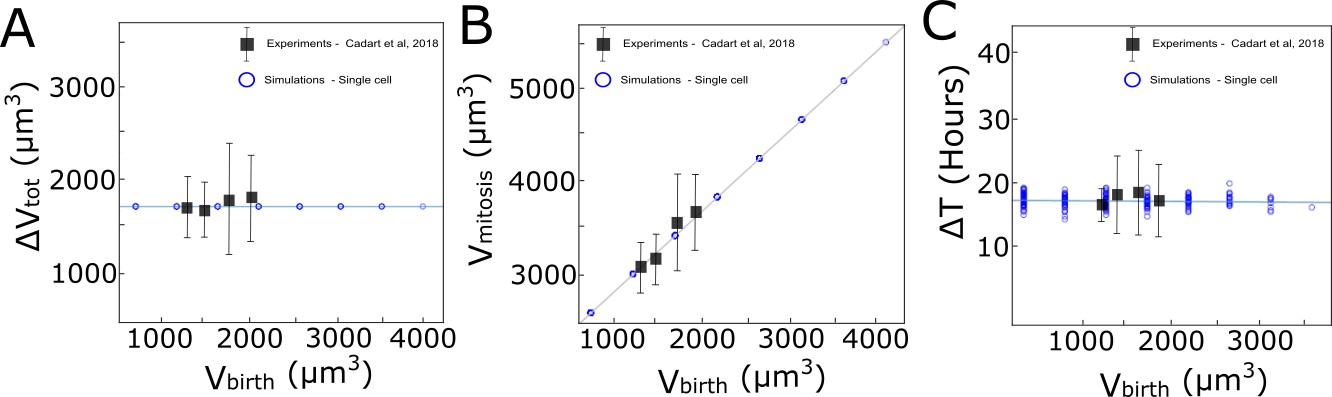
Computational implementation of the adder model of growth followed by MDCKWT cells.
The graphs show the relationship between (A) added volume ΔVtot during one cell cycle and volume at birth Vbirth, (B) the volume at mitosis Vmitosis and Vbirth, and (C) the cell cycle duration ΔTtot and Vbirth. Black squares: experimental data from Cadart et al., 2018. Blue circles: computational implementation of the adder model for single cells in our simulations. A similar set of rules was implemented for area assuming a constant cell height.
Figure 1—figure supplement 4
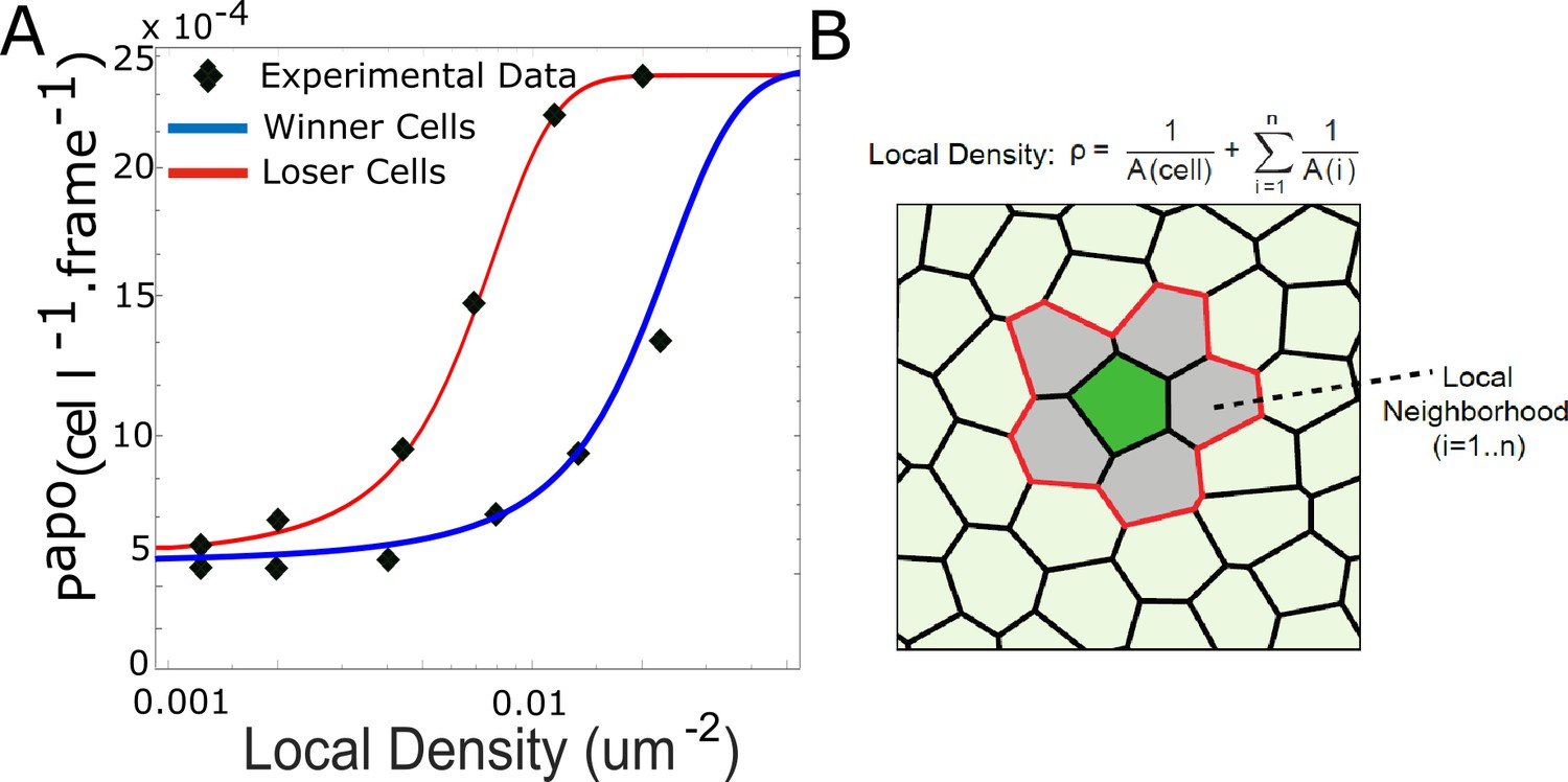
Density-dependent apoptosis.
(A) Probability of apoptosis as a function of local density for mechanical competition for winners (MDCKWT, blue) and losers (MDCKScrib, red). Markers denote experimental data for winner and loser cells from Bove et al., 2017. For winners and losers, the experimental data was fitted with the relationship: with ρ the local density. papo max was chosen to be the same for winners as for losers. (B) Definition of the local density ρ. The local cell density ρ for the cell of interest (green) was defined as the inverse of the sum of area of the cell of interest and its first neighbours (grey).
Figure 1—figure supplement 5
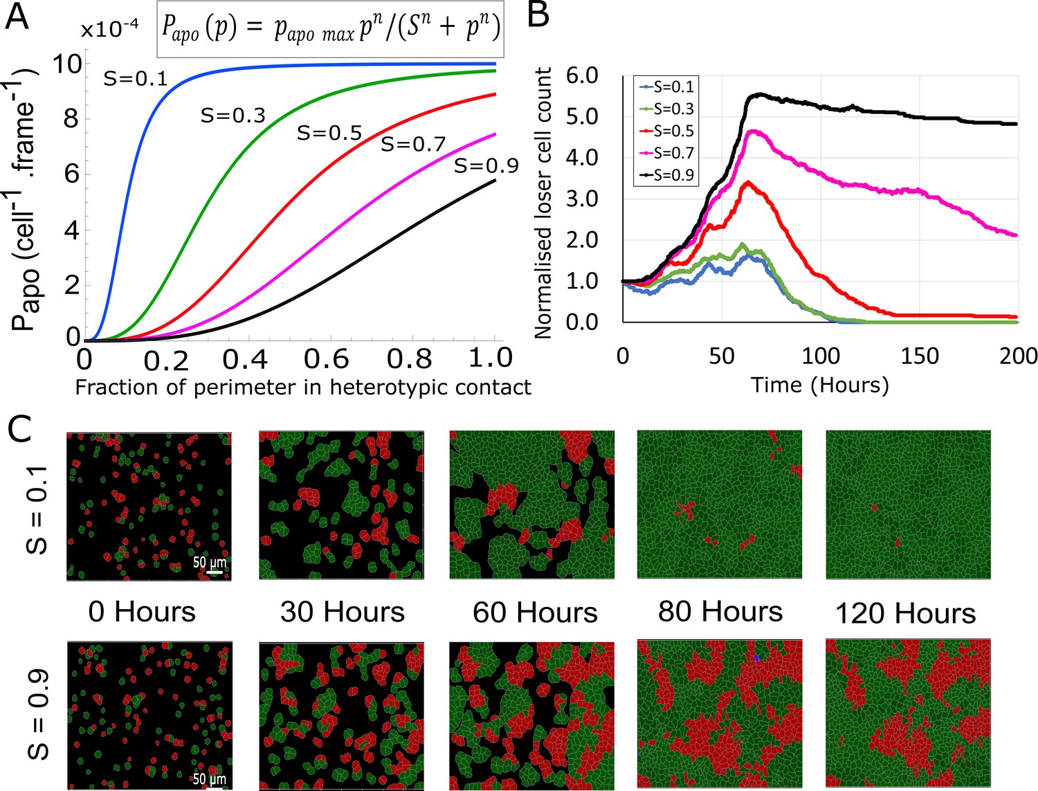
Contact-dependent apoptosis for biochemical competition.
(A) Probability of apoptosis as a function of the fraction of the perimeter p engaged in heterotypic contact. The probability of apoptosis is parametrised by a Hill function, whose equation is shown above the graph. S is the steepness parameter of the Hill function, p the fraction of the perimeter in heterotypic contact, and n = 3 was fixed in our simulations. (B) Evolution of normalised loser cell counts as a function of S with n = 3. (C) Simulation snapshots of biochemical competition initiated with 50% winner cells (green) and 50% loser cells (red). Dying cells are shown in blue. Top: for a low value of the steepness S of the Hill function, loser cells are rapidly eliminated. Bottom: for a high value of the steepness S, winners and losers coexist after 120 hr. See Video 6. (B, C) Parameters used for the simulations in this figure are in Supplementary file 3.
Figure 2 with 2 supplements
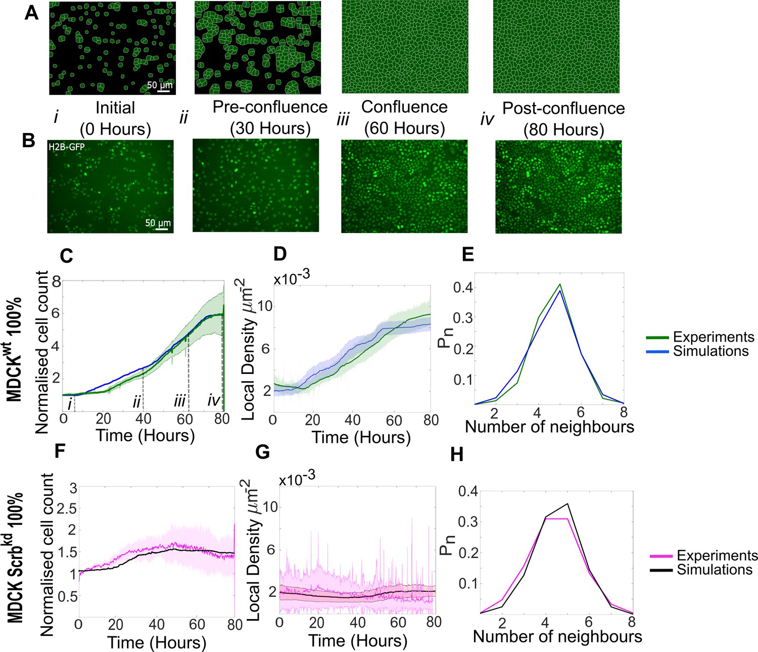
Model simulations capture the dynamics of growth and homeostasis in pure cell populations.
(A) Simulation snapshots of the growth of a pure population of winner cells (Video 1). Cells are initially separated by free space (black). Each image corresponds to one computational field of view, representing 530 µm × 400 µm. (B) Experimental snapshots of MDCKWT (winner) cells expressing the nuclear marker H2B-GFP (Video 2). Each image corresponds to 530 µm × 400 µm and is acquired by wide-field epifluorescence using ×20 magnification. The timing of each image is indicated between the two image rows. (C) Normalised cell count as a function of time for winner cells in simulations (blue) and MDCKWT experiments (green). (i–iv) indicate the time points at which the snapshots in (A, B) were taken. (D) Average local cellular density as a function of time for the same data as (C). (E) Distribution of sidedness of cells post confluence. The curves indicate the proportion of cells as a function of number of neighbours. (C–E) Green curves represent experimental data and blue curves simulated data. (F–H) are same as (C–E) for pure populations of loser cells (MDCKScrib). Magenta curves are experimental data (Video 3), and black curves represent simulated data. (C–H) Data are pooled from three biological replicates imaging four fields of view each and from 12 simulations. The solid line indicates the mean, and the shaded area indicates the standard deviation. Parameters used for the simulations in this figure are listed in Supplementary file 1.
Figure 2—figure supplement 1
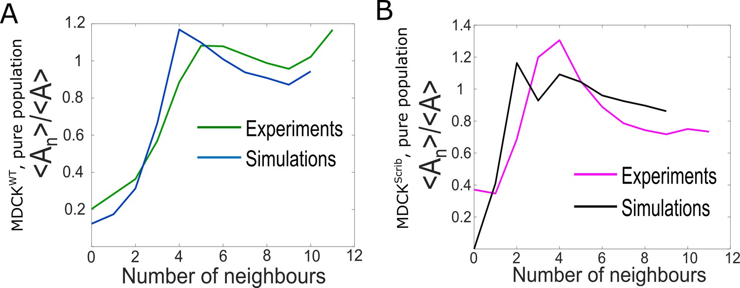
Comparison of epithelium organisation in simulations and experiments for pure populations.
(A) Ratio of the average area of cells with n neighbours <An> to the average area of all cells <A> as a function of number of neighbours for winner cells. The green line represents experiments and the blue line simulations. (B) Ratio of the average area of cells with n neighbours <An> to the average area of all cells <A> as a function of number of neighbours for loser cells. The pink line represents experiments and the black line simulations.
Figure 2—figure supplement 2
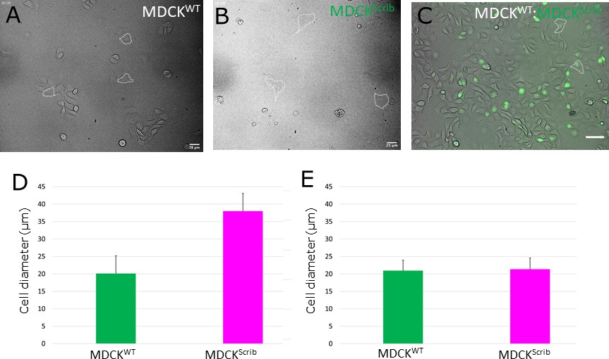
Cell area in pure and mixed populations prior to confluence.
Brightfield images of isolated winner cells (A) and loser cells (B) in pure populations. (A, B) Scale bars = 25 µm. Representative cell areas are outlined in dashed white lines. (C) Brightfield image of winner cells and loser cells in mixed populations. Loser cells are indicated by their green nuclei acquired using H2B-GFP fluorescence. Representative loser cells are outlined in dashed white lines. Scale bar = 50 µm. (D) Effective cell diameter for MDCKWT and MDCKScrib cells in pure populations. (E) Effective cell diameter for MDCKWT and MDCKScrib cells in mixed populations. (D, E) These measurements are used to parametrise the cell size at birth AT(0) and the area added in each cell cycle . Error bars represent the standard deviation.
Figure 3
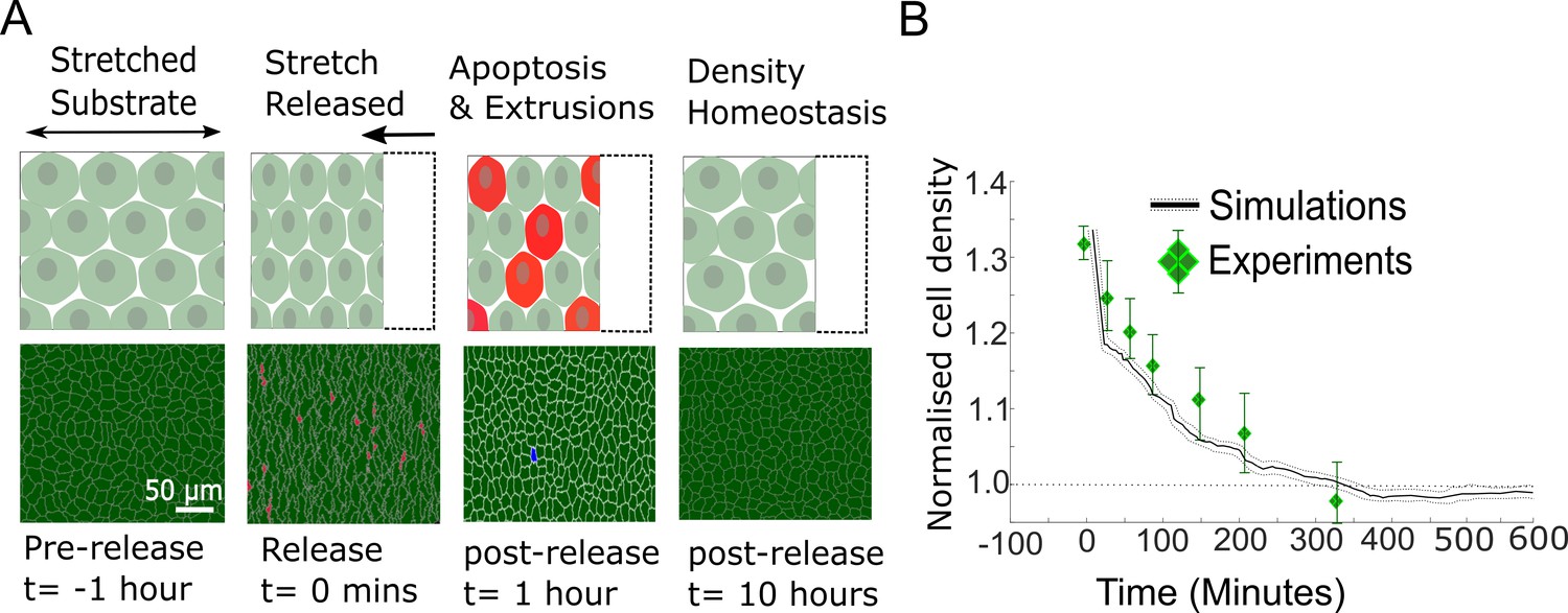
Model epithelia return to homeostasis in response to a sudden increase in local density.
(A) Winner cells grown to confluence on a stretched silicon substrate are subjected to a sudden increase in density after stretch release. The monolayer returns to its homeostatic density over time through extrusions and density-mediated apoptoses. Top row: cartoon diagrams depicting the experiment. Bottom row: snapshots of simulations. Cells eliminated by live cell extrusion are shown in red and by apoptosis in blue. (B) Evolution of cell density as a function of time in response to a step increase in cell density at t = 0 min. Density in simulations is indicated by the black line, and experimental data from Eisenhoffer et al., 2012 are shown by green diamond markers. The shaded region around the black line indicates the standard deviation of n = 5 simulations. The whiskers around the diamond markers indicate the standard deviation of the experimental measurements. The dashed horizontal line denotes the initial cell density.
Figure 4 with 1 supplement
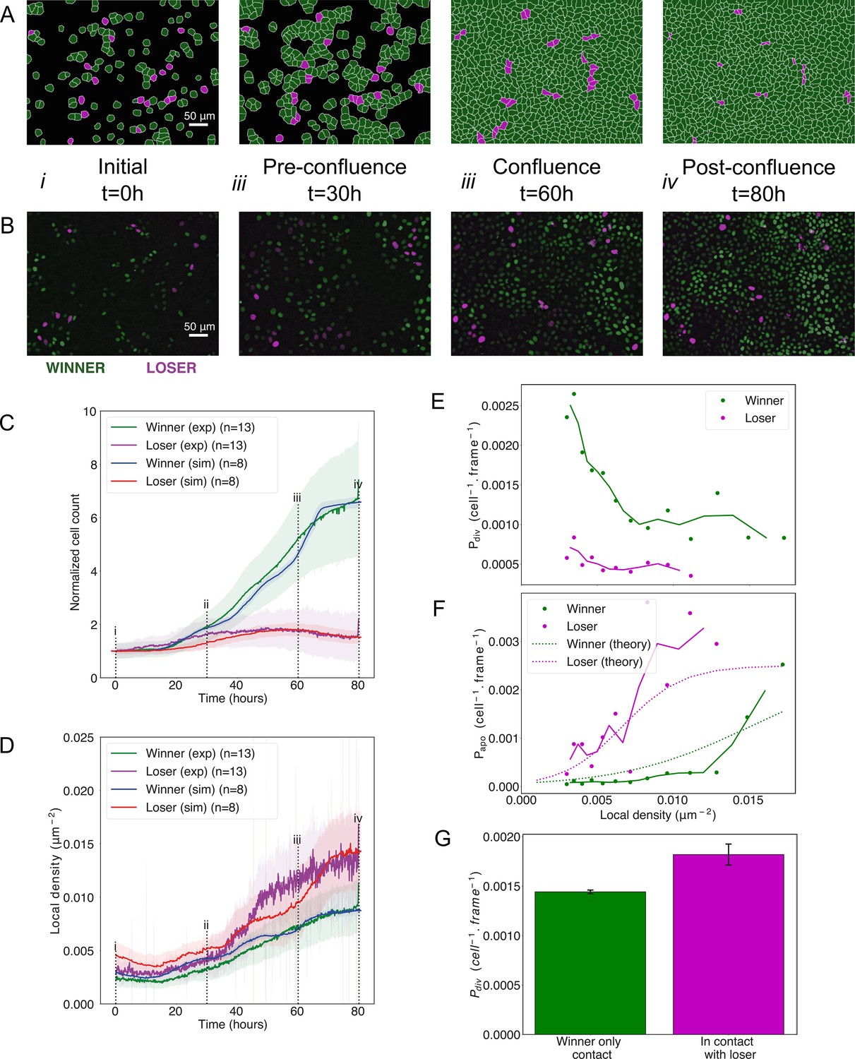
Cell competition in co-cultures of cells with different homeostatic densities.
(A) Simulation snapshots of competition between 90% winner (green) and 10% loser cells (red) (Video 4). Cells are initially separated by free space (black). Each image corresponds to 530 µm × 400 µm. (B) Experimental snapshots of competition between 90% MDCKWT cells (winner, green) and 10% MDCKScrib cells (loser, red) (Video 5). MDCKWT express the nuclear marker H2B-GFP, while MDCKScrib express the nuclear marker H2B-RFP. Each image corresponds to 530 µm × 400 µm and is acquired by wide-field epifluorescence using ×20 magnification. The timing of snapshots is indicated in between rows A and B. Scale bars represent 50 µm. (C) Temporal evolution of normalised cell count for winner cells (simulations: blue line; experiments: green line) and loser cells (simulations: red line; experiments: purple line) in experiments and simulations initiated with a 90:10 ratio of winner:loser cells. Data are pooled from three biological replicates imaging four fields of view for the experiments and from 12 simulations. (i–iv) indicate the time points at which the snapshots in (A, B) were taken. (D) Temporal evolution of the local cell density for the simulations and experiments shown in (C). The local density is defined in Figure 1—figure supplement 4B. (C, D) Solid lines indicate the average of the data, and the shaded area indicates the standard deviation. (E) Probability of division per cell per frame as a function of local density predicted from simulations. Markers indicate probability of division for each density bin, and solid lines indicate moving average. (F) Probability of apoptosis per cell per frame as a function of local density predicted from simulations compared to the theoretical input functions implemented in the model. Markers indicate probability of apoptosis for each density bin, and solid lines indicate moving average. Dashed lines show the input functions implemented in the model based from experimental data in Bove et al., 2017; Figure 1—figure supplement 4A. (G) Probability of division per cell per frame for winner cells in contact with winner only (green bar) and in contact with at least one loser cell (red bar). Whiskers indicate the coefficient of variation cv calculated for each. The number of cells observed N and number of divisions n were respectively N = 4.3×10⁶ and n = 6246 for winner contact only and N = 1.6 105 and n = 292 for winners in contact with losers. Data was gathered from 10 simulations. Parameters used for the simulations in this figure are in Supplementary file 1.
Figure 4—figure supplement 1
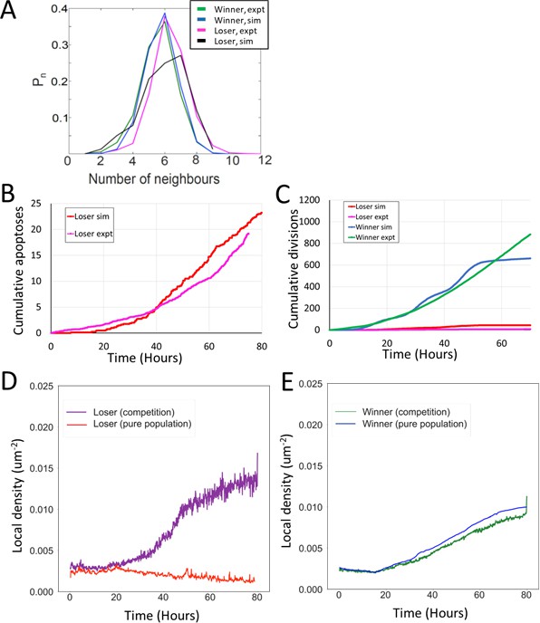
Comparison between simulations and experiments for mechanical competition.
(A) Sidedness of cells post confluency for mechanical competition shown in Figure 4A. The curves indicate the proportion of cells as a function of number of neighbours. The green curve corresponds to winner cells in experiments, the blue to winner cells in simulations, the magenta to loser cells in experiments, and the black to loser cells in simulations. (B) Average cumulative apoptoses during mechanical competition for loser cells. The red curve indicates simulations and the magenta curve experiments. (C) Average cumulative divisions during mechanical competition. Experiments for winner cells are shown in green and simulations in blue. Experiments for loser cells are shown in magenta and simulations in red. (B, C) Data averaged over eight simulations and eight experiments. (D) Evolution of average local density in loser cells in pure populations (red) and in competition (purple). (E) Evolution of average local density in winner cells in pure populations (blue) and in competition (green). (D, E) Data from Figures 2D and 4D.
Figure 5 with 1 supplement

Cellular stiffness and homeostatic density control the outcome of mechanical competition.
(A) Evolution of homeostatic density as a function of the parameter k, quantifying the sensitivity to contact inhibition. Data are shown for pure populations of winner (blue) and loser (red) cells. (B) Simulation snapshots of competition between 90% winner cells (green) and 10% loser cells (red). The top two panels show the population evolution for a small difference in homeostatic density ΔHD between the two cell types. The bottom two panels show the population evolution for a large ΔHD between the two cell types. Winner cells are shown in green and loser cells in red. Each image corresponds to 530 µm × 400 µm. (C) Normalised cell count for loser cells in competition simulations for different values of the contact inhibition parameter k in the winner cells. As k decreases, ΔHD increases. Temporal evolution of cell count in longer simulations is shown in Figure 5—figure supplement 1D. (D) Normalised cell count for loser cells in competition simulations for different values of the relative stiffness parameter . Winner cells have a fixed stiffness of 1.0. Temporal evolution of cell count in longer simulations is shown in Figure 5—figure supplement 1E. Snapshots of competition are shown in Figure 5—figure supplement 1F, G for Λ = 0.3 and Λ = 2. (E) Loser cell survival fraction after 80 hr in simulations run with different parameters for relative stiffness Λ (red line) and contact inhibition k (blue line). Shaded blue and red regions denote the standard deviation. The grey shaded region indicates the survival fraction of loser cells observed in experiments after 80 hr. The x-axis scale is indicated on the top of the graph for Λ and on the bottom of the graph for k. (F) Time to 50% elimination of loser cells as a function of the contact inhibition parameter. The solid line indicates the mean and the shaded regions the standard deviation. Parameters used for the simulations in this figure are in Supplementary file 2.
Figure 5—figure supplement 1
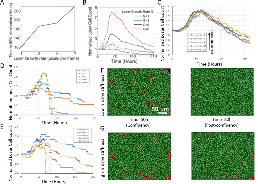
Effect of simulation parameters on mechanical competition.
(A) Time to 50% elimination of loser cells in mechanical competition as a function of loser growth rate. Winner cell growth rate was set to 6.0. (B) Normalised loser cell count in mechanical competition as a function of time for different values of loser cell growth rate. Winner cell growth rate was set to 6.0. (C) Evolution of normalised loser cell count for different values of JHeterotypic. In our simulations, the heterotypic adhesion energy JHeterotypic = 1 is the most adhesive, and JHeterotypic = 20 is the least adhesive. Average of three simulations for each curve. (D) Evolution of normalised loser cell count for different values of the contact inhibition parameter k. One simulation per curve. (E) Evolution of normalised loser cell count for different values of the stiffness λ. One simulation per curve. Winner cell stiffness was set to 1. (F, G) Simulation snapshots of a competition initiated with 90% winner cells (green) and 10% loser cells (red) for different relative stiffnesses . (F) Population evolution for a low loser relative stiffness (Λ = 0.3). (G) Population evolution for a high loser relative stiffness (Λ = 2). (A–G) Parameters used for the simulations in this figure are in Supplementary file 2.
Figure 6 with 2 supplements
Tissue organisation governs the outcome of biochemical competition.
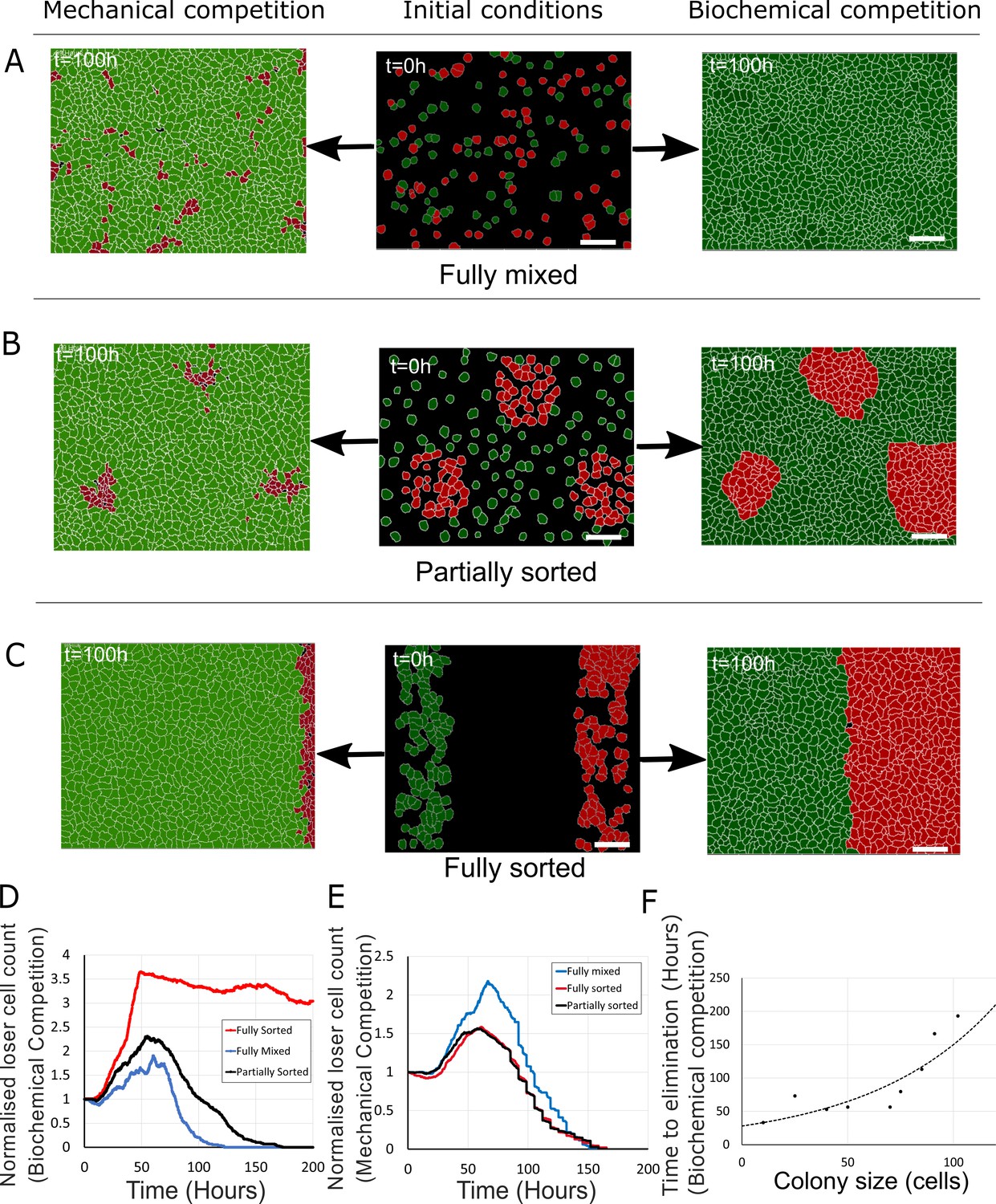
(A–C) The middle panels show the initial configuration of a competition between 50% loser (red) and 50% winner (green) cells for various seeding arrangements (A: fully mixed; B: partially sorted; C: fully sorted). The right panels show a representative outcome for biochemical competition. The left panels show a representative outcome for mechanical competition. Cells are initially separated by free space (black). (D) Normalised loser cell count for the three configurations for biochemical competition (A–C, right-hand column). (E) Normalised loser cell count for the three configurations for mechanical competition (A–C, left-hand column). (D, E) Loser cell count for each configuration was averaged over three simulations. (F) Time to elimination as a function of the size of loser cell colonies for biochemical competition. Markers indicate the time determined in simulations for each colony size (N = 1 simulation for each colony size). The dashed line is a fit to an exponential function of the form Ae-t/τ, r2 = 0.73 and τ ~ 60 hr. Parameters used for the biochemical simulations in this figure are in Supplementary file 3.
Figure 6—figure supplement 1
Tissue organisation and heterotypic adhesion influence the outcome of competition in biochemical competition.
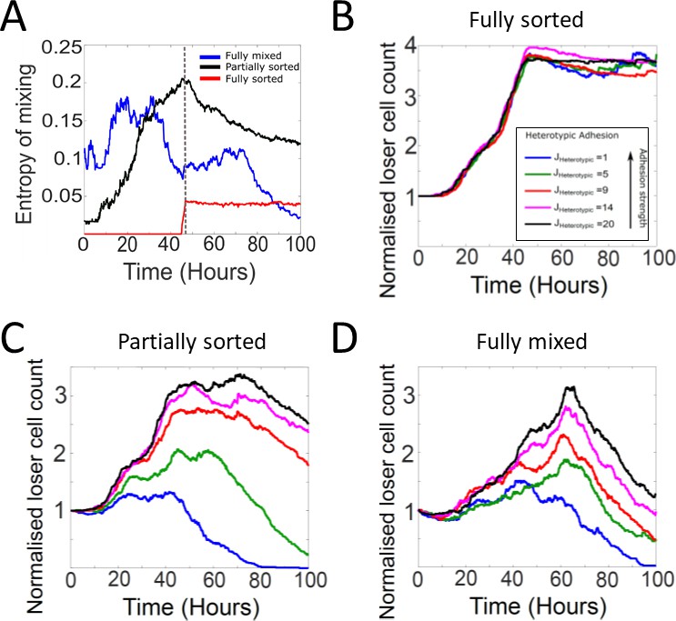
(A) Temporal evolution of the entropy of cell mixing for three different initial configurations for biochemical competition (see Figure 6A–C). The dashed line indicates the time at which the epithelium reaches confluence. (B–D) Heterotypic adhesion was varied from JHeterotypic = 1–20. In our simulations, the heterotypic adhesion energy JHeterotypic = 1 is the most adhesive, and JHeterotypic = 20 is the least adhesive. Homotypic adhesion energy is fixed to JHomotypic = 8. The colour code is given in the bottom-right corner of panel (B). (B) Normalised loser cell counts for different values of heterotypic adhesion between winner and loser cells starting from a fully sorted configuration (Figure 6B). (C) Normalised loser cell counts for different values of heterotypic adhesion between winner and loser cells starting from a partially sorted configuration (Figure 6B). (D) Normalised loser cell counts for different values of heterotypic adhesion between winner and loser cells starting from a fully mixed configuration (Figure 6A). (B–D) Parameters used for the simulations in this figure are in Supplementary file 3.
Figure 6—figure supplement 2
Mechanical competition experiments in partially sorted starting conditions.
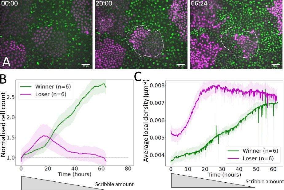
(A) Experimental snapshots of a mechanical competition initiated with MDCKScrib (losers, magenta) surrounded by MDCKWT cells (winners, green) in a partially sorted configuration. Dashed white lines indicate the outline of one colony at the onset of competition at t = 0 hr. Silencing of scribble was induced 24 hr before the start of imaging, and the amount of protein decreases progressively over the course of the experiment (Norman et al., 2012). Scale bar 25 µm. Time is indicated in hours and minutes in the top-left corner of each snapshot. (B) Normalised cell count for winners (green) and losers (magenta) in a competition starting from a partially sorted configuration. (C) Average local density for winner and loser cells in a competition starting from a partially sorted configuration. (B, C) Solid lines indicate the average of six experiments. The shaded area indicates the standard deviation. An approximate time course of scribble amount is depicted below the graph based on experimental data from Norman et al., 2012.
Videos
Video 1
Simulation of the growth of a pure winner cell epithelium (Figure 2A).
Video 2
Representative growth of a pure MDCKWT epithelium over 66 hr (Figure 2B).
The nucleus of MDCKWT cells is labelled with H2B-GFP. Scale bar 25 µm.
Video 3
Representative growth of a pure MDCKScrib epithelium over 79 hr (Figure 2F–H).
The nucleus of MDCKScrib cells is labelled with H2B-mRFP. Scale bar 25 µm.
Video 4
Simulation of mechanical competition between 90% winner cell types and 10% loser cell types for default parameters (Figure 4A, C, D).
The different shades of green represent the different generations of winner cells, and the different shades of red represent the different generations of loser cells.
Video 5
Representative competition between 90% MDCKWT and 10% MDCKScrib over 66 hr (Figure 4B–D).
MDCKWT nuclei are marked with H2B-GFP (green), and MDCKScrib nuclei are marked with H2B-mRFP (magenta). Scale bar 25 µm.
Video 6
Simulation of biochemical competition between 50% winner cell types and 50% loser cell types in an initial fully mixed configuration for a low value of the steepness S = 0.1 (Figure 1—figure supplement 5C).
Video 7
Simulation of biochemical competition between 50% winner cell types and 50% loser cell types in an initial partially sorted configuration (Figure 6B).
Video 8
Simulation of mechanical competition between 50% winner cell types and 50% loser cell types in an initial partially sorted configuration (Figure 6B).
Video 9
Representative experiment of a competition between MDCKWT cells and MDCKScrib cells in a partially sorted initial configuration.
MDCKWT nuclei are marked with H2B-GFP (green), and MDCKScrib nuclei are marked with H2B-mRFP (magenta). The movie represents 66 hr. Scale bar 50 µm.
Video 10
Simulation of biochemical competition between 50% winner cell types and 50% loser cell types in an initial fully sorted configuration (Figure 6C).
Additional files
-
Supplementary file 1
Table of default parameters for mechanical competition in Figures 2 and 4.
Parameters for the Potts model are shaded in grey. Initial conditions and computational implementation parameters are in white. Cell automaton parameters are in pink. Probability of apoptosis is implemented by a function of the form . A.u.: arbitrary units.
- https://cdn.elifesciences.org/articles/61011/elife-61011-supp1-v1.xlsx
-
Supplementary file 2
Table of parameters for investigating the control of mechanical competition in Figure 5 and Figure 5—figure supplement 1.
Parameters for the Potts model are shaded in grey. Initial conditions and computational implementation parameters are in white. Cell automaton parameters are in pink. Parameters that were varied are indicated, and the range is given in brackets. Probability of apoptosis is implemented by a function of the form . A.u.: arbitrary units.
- https://cdn.elifesciences.org/articles/61011/elife-61011-supp2-v1.xlsx
-
Supplementary file 3
Table of parameters for investigating the control of biomechanical competition in Figure 6 and Figure 1—figure supplement 5.
Parameters for the Potts model are shaded in grey. Initial conditions and computational implementation parameters are in white. Cell automaton parameters are in pink. Parameters that were varied are indicated, and the range is given in brackets. Probability of apoptosis is implemented by a Hill function of the form with p the fraction of perimeter occupied by heterotypic adhesions. A.u.: arbitrary units.
- https://cdn.elifesciences.org/articles/61011/elife-61011-supp3-v1.xlsx
-
Supplementary file 4
Table of parameters investigated in simulations of mechanical competitions: fixed parameters.
See Supplementary files 1 and 2 for exact values.
- https://cdn.elifesciences.org/articles/61011/elife-61011-supp4-v1.xlsx
-
Supplementary file 5
Table of parameters investigated in simulations of biochemical competitions: fixed parameters.
See Supplementary file 3 for exact values. Note that all density-related parameters are fixed because apoptosis does not depend on density.
- https://cdn.elifesciences.org/articles/61011/elife-61011-supp5-v1.xlsx
-
Transparent reporting form
- https://cdn.elifesciences.org/articles/61011/elife-61011-transrepform-v1.docx
Download links
A two-part list of links to download the article, or parts of the article, in various formats.
Downloads (link to download the article as PDF)
Open citations (links to open the citations from this article in various online reference manager services)
Cite this article (links to download the citations from this article in formats compatible with various reference manager tools)
Cell-scale biophysical determinants of cell competition in epithelia
eLife 10:e61011.
https://doi.org/10.7554/eLife.61011


