Impaired adaptation of learning to contingency volatility in internalizing psychopathology
- Department of Psychology, UC Berkeley, United States
- Max Planck Institute for Biological Cybernetics, Germany
- Max Planck Institute for Human Development, Germany
- University of Tübingen, Germany
- Wellcome Centre for Integrative Neuroimaging, University of Oxford, FMRIB, John Radcliffe Hospital, United Kingdom
- Helen Wills Neuroscience Institute, UC Berkeley, United States
Figures
Figure 1 with 2 supplements
Bifactor analysis of internalizing symptoms.
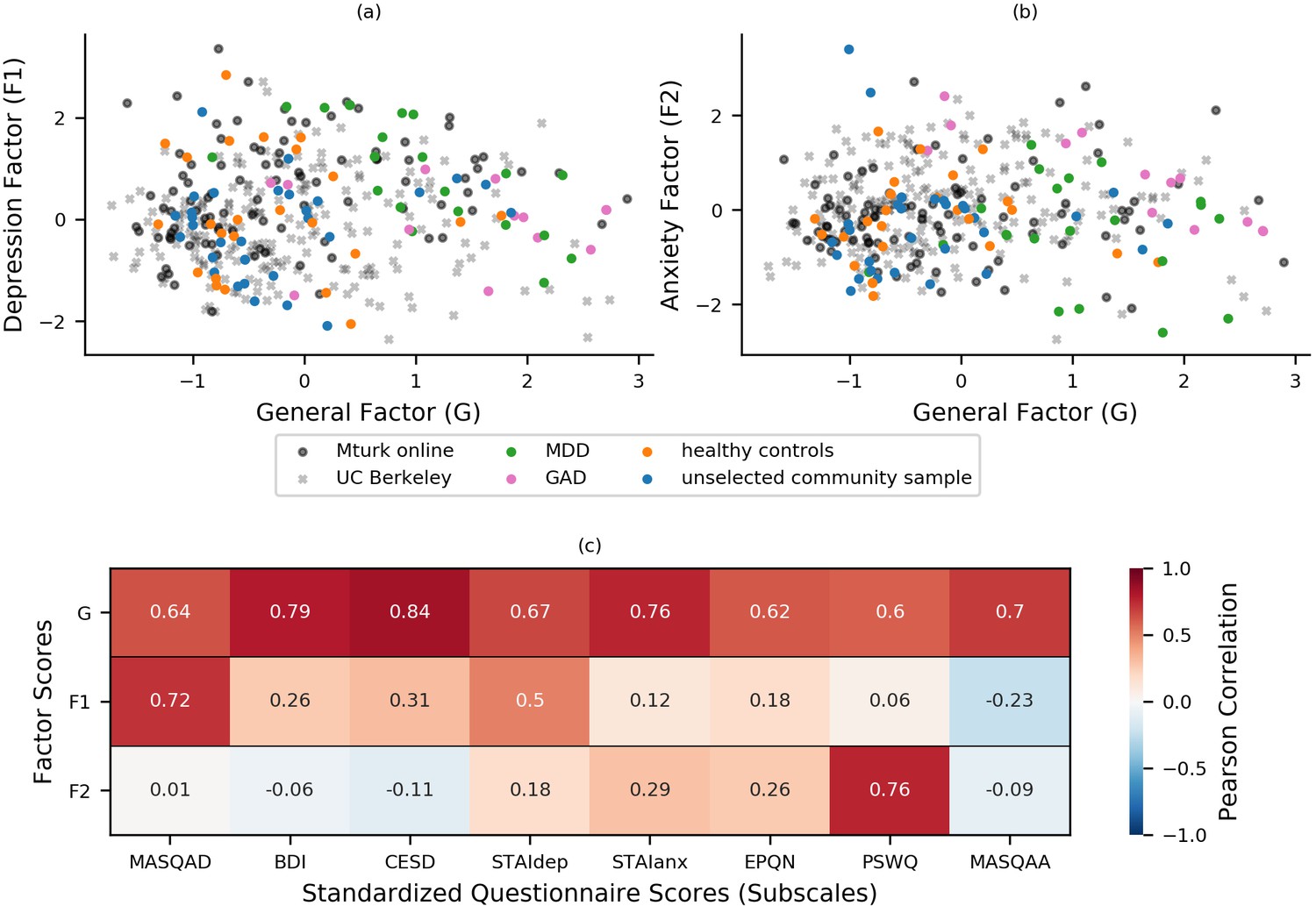
(a-b) Bifactor analysis of item-level scores from the STAI, BDI, MASQ, PSWQ, CESD, and EPQ-N (128 items in total) revealed a general ‘negative affect’ factor (xaxis) and two specific factors: one depression-specific (left panel, y-axis) and one anxiety-specific (right panel, y-axis). The initial bifactor analysis was conducted in a sample (n = 86) comprising participants diagnosed with MDD, participants diagnosed with GAD, healthy control participants and unselected community participants. The factor solution showed a good fit in a separate sample of participants (n = 199) recruited and tested online through UC Berkeley’s participant pool (x). Item loadings on a sub-set of questionnaires were used to calculate factor scores for a third set of participants recruited and tested online through Amazon’s Mechanical Turk (n = 147), see Experiment 2. It can be seen that both online samples show a good range of scores across the general and two specific factors that encompass the scores shown by patients with GAD and MDD. (c) Factor scores were correlated with summary scores for questionnaire scales and subscales to assess the construct validity of the latent factors. This was conducted using a combined dataset comprising data from both the exploratory (n = 86) and confirmatory (n = 199) factor analyses. Scores on the general factor correlated highly with all questionnaire summary scores, scores on the depression-specific factor correlated highly with measures of depression, especially anhedonic depression, and scores on the anxiety-specific factor correlated particularly highly with scores for the PSWQ. MASQAD = Mood and Anxiety Symptoms Questionnaire (anhedonic depression subscale); BDI = Beck Depression Inventory; CESD = Center for Epidemiologic Studies Depression Scale; STAIdep = Spielberger State-Trait Anxiety Inventory (depression subscale); STAIanx = Spielberger State-Trait Anxiety Inventory (anxiety subscale); EQN-N = Eysenck Personality Questionnaire (Neuroticism subscale); PSWQ = Penn State Worry Questionnaire; MASQAA = Mood and Anxiety Symptoms Questionnaire (anxious arousal subscale); MDD = major depressive disorder; GAD = generalized anxiety disorder.
Figure 1—figure supplement 1

Scree plot for the eigenvalue decomposition of the covariance matrix of individual items from the battery of internalizing symptom measures.
Bifactor analysis was applied to the item-level scores from the STAI, BDI, MASQ, PSWQ, CESD, and EPQ-N (128 items in total) for participants in experiment 1. Prior to the estimation of the bifactor model, eigenvalue decomposition of the covariance matrix of individual items was used to inform the decision of how many factors to include in the model. A ‘scree’ plot for the eigenvalue decomposition of the covariance matrix is shown. The location of the elbow in this plot, along with the parallel analysis, which compares the sequence of eigenvalues from the data to their corresponding eigenvalues from a random normal matrix of equivalent size (Horn, 1965; Humphreys and Montanelli, 1975; Floyd and Widaman, 1995), suggests that there were three dimensions of symptom variation that were distinguishable from noise. STAI = Spielberger State-Trait Anxiety Inventory; BDI = Beck Depression Inventory; MASQ = Mood and Anxiety Symptoms Questionnaire; PSWQ = Penn State Worry Questionnaire; CESD = Center for Epidemiologic Studies Depression Scale; EQN-N = Eysenck Personality Questionnaire (Neuroticism subscale); MDD = major depressive disorder; GAD = generalized anxiety disorder.
Figure 1—figure supplement 2
Correlation matrices for internalizing questionnaire scales and latent factors from the bifactor analysis.
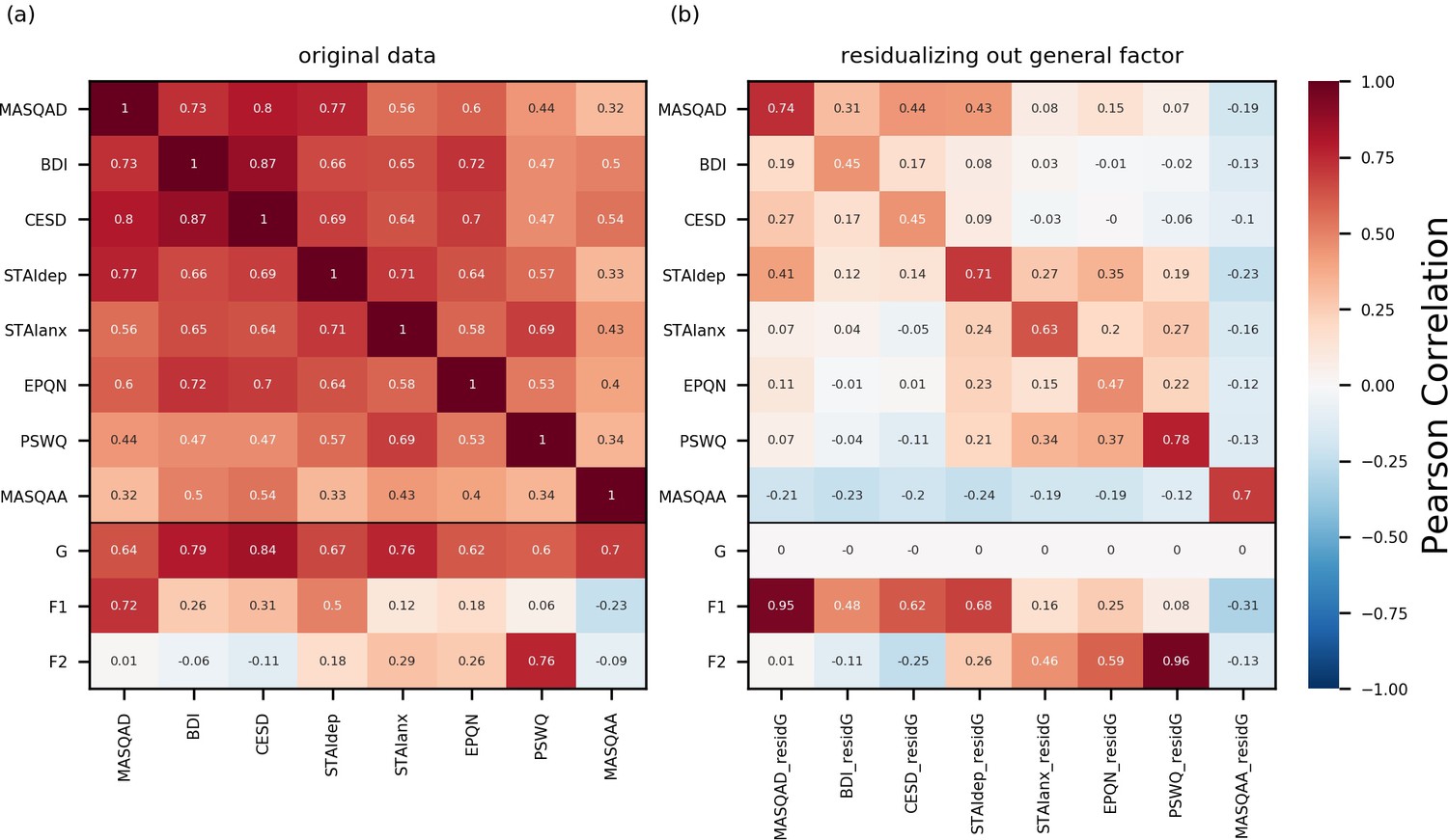
(a) We calculated summary scores for each participant for each of the standardized questionnaires we administered. All participants who completed the full set of questionnaires were included: this comprised both participants in experiment 1 (n = 86) and participants whose data was used for the confirmatory factor analysis (n = 199). Full scale scores were used for the Beck Depression Inventory (BDI), the Center for Epidemiologic Studies Depression Scale (CESD), and the Penn State Worry Questionnaire (PSWQ), and subscale scores were used for the Spielberger Trait Anxiety Inventory (anxiety and depression subscales: STAIanx, STAIdep), the Eysenck Personality Questionnaire (neuroticism subscale: EPQ-N) and the Mood and Anxiety Symptoms Questionnaire (anhedonic depression and anxious arousal subscales: MASQ-AD, MASQ-AA). Participants’ scores for these measures were correlated with their scores for the three latent factors (G = general factor; F1 = depression-specific factor; F2 = anxiety-specific factor). The resultant correlations are given in panel (a) (see Materials and methods for further details). (b) Here, we have regressed variance explainable by general factor scores out from each (sub)scale and participants’ residual scores are correlated against their latent factor scores as well as their scores on the questionnaire scales without variance explained by the general factor removed. The magnitude of correlation between participants’ residual scores for a given scale and their original, non-residualized, scores for that scale reveals how much variance in scores for that measure cannot be explained by the general factor. These correlations were highest for the MASQ-anhedonia subscale (MASQ-AD; r = 0.74) and the Penn-State Worry Questionnaire (PSWQ; r = 0.78), with approximately 50% of score variance (the square root of the correlation) not being captured by the general factor. Nearly all this residual variance could be explained by scores on the specific factors. MASQ-AD residual scores (MASQAD_residG) and scores on the depression specific factor (F1) showed a correlation of r = 0.95; PSWQ residual scores (PWSQ_residG) and scores on the anxiety-specific factor (F2) showed a correlation of r = 0.96. These correlational results speak to the content validity of the three latent factors with the general factor explaining variance across both measures of anxiety and depression, the anxiety-specific factor capturing additional variance unique to anxiety measures and the depression-specific factor capturing additional variance unique to depression measures.
Figure 2
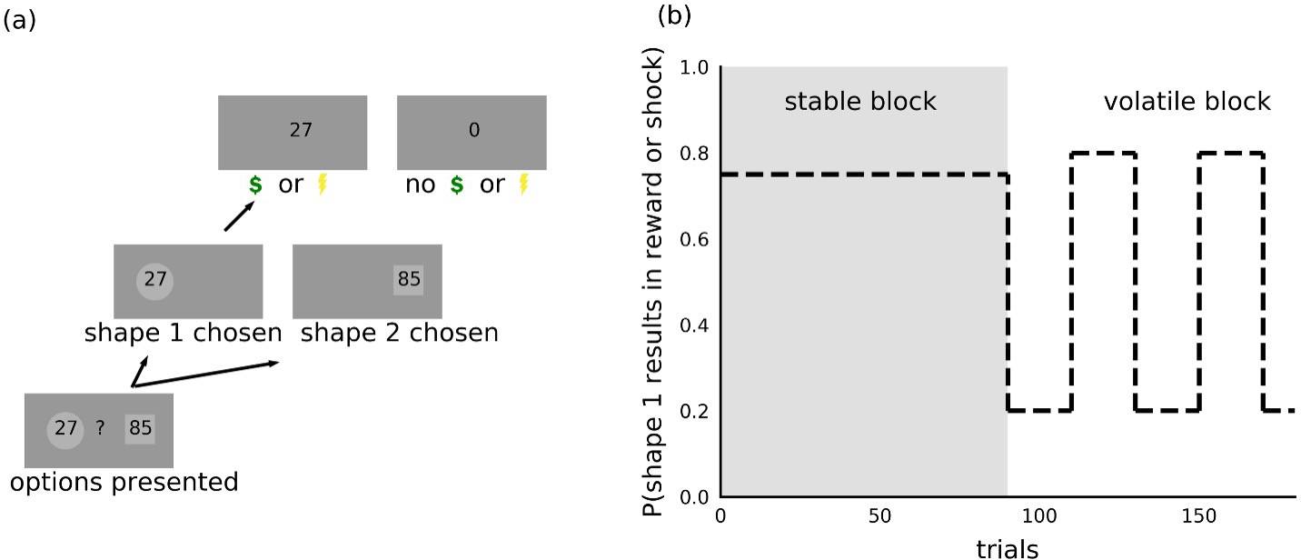
Task.
(a) On each trial, participants chose between two shapes. One of the two shapes led to receipt of shock or reward on each trial, the nature of the outcome depending on the version of the task. The magnitude of the potential outcome was shown as a number inside each shape and corresponded to the size of the reward in the reward version of the task or intensity of the electric shock in the aversive version of the task. (b) Within each task, trials were organized into two 90-trial blocks. During the stable block, one shape had a 75% probability of resulting in reward or shock receipt; the other shape resulted in shock or reward receipt on the remaining trials. During the volatile block, the shape with the higher probability (80%) of resulting in shock or reward receipt switched every 20 trials. Participants were instructed to consider the magnitude of the potential outcome, shown as a number inside each shape, as well as the probability that the outcome would occur if the shape was chosen.
Figure 3
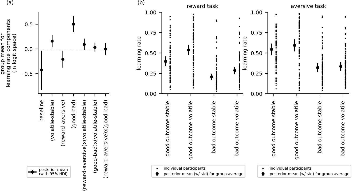
Cross-group results from experiment 1 for effects of block type (volatile, stable), task version (reward, aversive), and relative outcome value (good, bad) on learning rate (n = 86).
(a) This panel shows the posterior means along with the 95% highest posterior density intervals (HDI) for the group means () for each learning rate component (i.e. for baseline learning rate and the change in learning rate as a function of each within-subject factor and their two-way interactions). The 95% posterior intervals excluded zero for effect of block type upon learning rate (i.e. difference in learning rate for the volatile versus stable task blocks ). This was also true for the effect of task version, that is, whether outcomes entailed reward gain or electrical stimulation () and for the effect of relative outcome value, that is, whether learning followed a relatively good (reward or no stimulation) or relatively bad (stimulation or no reward) outcome (. Participants showed higher learning rates during the volatile block than the stable block, during the aversive task than the reward task, and on trials following good versus bad outcomes. None of the two-way interactions were statistically credible, that is the 95% posterior included zero. (b) In this panel, the learning rate components are combined to illustrate how learning rates changed across conditions. The posterior mean learning rate for individual participants (small dots) and the group posterior mean learning rate (large dots, error bars represent the associated posterior standard deviation) are given for each of the eight conditions; these values were calculated from the posterior distributions of the learning rate components ( etc.) and the group means ().
Figure 4 with 1 supplement
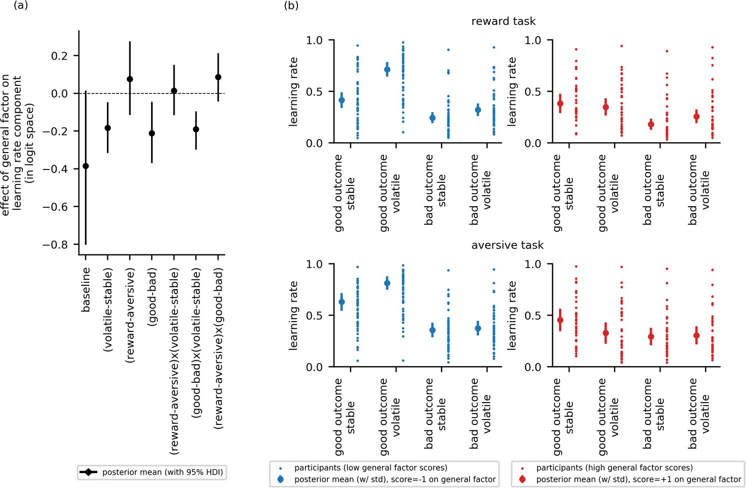
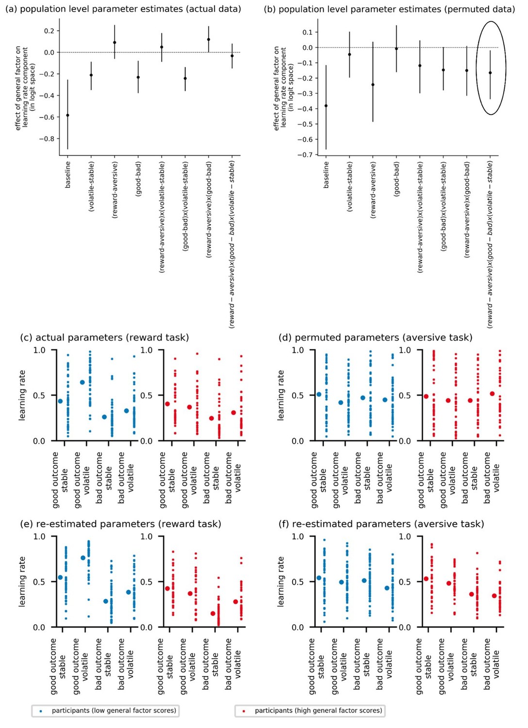
Experiment 1: Effect of general factor scores on learning rate (in-lab sample, n = 86).
Panel (a) shows posterior means and 95% highest posterior density intervals (HDI) for the effect of general factor scores () on each of the learning rate components. General factor scores credibly modulated the extent to which learning rate varied between the stable and volatile task blocks ( = −0.18, 95%-HDI = [−0.32,–0.05]), the effect of relative outcome value on learning rate ; = −0.21, 95%-HDI = [−0.37,–0.04]) and the interaction of these factors upon learning rate (; = −0.19, 95%-HDI = [−0.3,–0.1]). In each case, the 95% HDI did not include 0. (b) Here, we illustrate learning rate as a function of each within-subject factor and high versus low scores on the general factor of internalizing symptoms. To do this, we calculated the expected learning rate for each within-subject condition associated with scores one standard deviation above (‘high’, shown in red) or below (‘low’, shown in blue) the mean on the general factor. It can be seen that the largest difference in learning rates for participants with high versus low general factor scores is on trials following good outcomes during volatile task blocks. This effect is observed across both reward and aversive task versions. Small data points represent posterior mean parameter estimates for individual participants. Large points represent the posterior mean learning rates expected for participants with scores ± 1 standard deviations above or below the mean on the general factor. Error bars represent the posterior standard deviation for these expected learning rates.
Figure 4—figure supplement 1
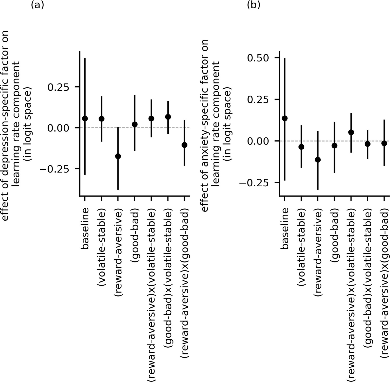
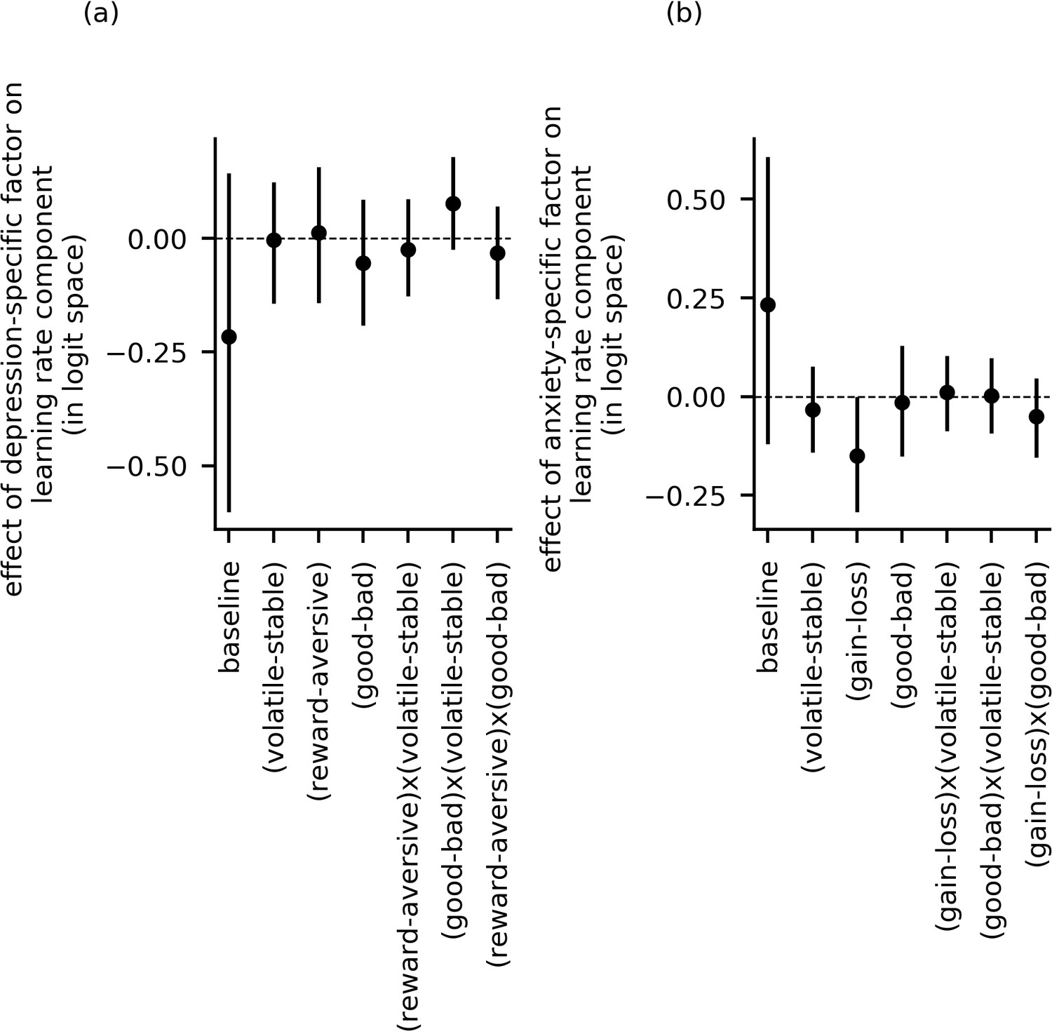
Effect of depression-specific and anxiety-specific factors on learning rate and its components (data from experiment 1).
Panel (a) and panel (b) show the effects of depression-specific factor scores and anxiety-specific factor scores, respectively, on each of the learning rate components (e.g. ). The 95%-HDI’s for population-level parameters and included zero for all parameter components. This indicates that neither depression-specific nor anxiety-specific factor scores credibly modulated learning rate as a function of block type (volatile versus stable), task version (reward versus aversive), or relative outcome value (good versus bad), or as a function of any of the two-way interactions of these experimental factors.
Figure 5 with 2 supplements
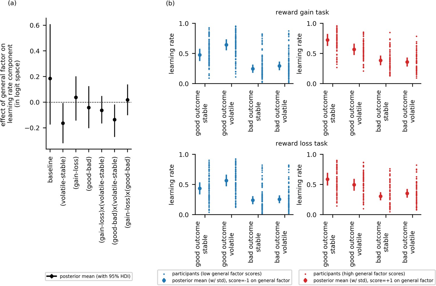
Experiment 2: Effect of the general factor scores on learning rate (online sample, n = 147).
Panel (a) shows posterior means and 95% highest posterior density intervals (HDI) for the effect of general factor scores () on each of the learning rate components. Replicating findings from experiment 1, general factor scores credibly modulated the extent to which learning rate varied between the stable and volatile task block ( = −0.16, 95%-HDI = [−0.32,–0.01]) and the extent to which this in turn varied as a function of relative outcome value ( = −0.14, 95%-HDI = [−0.27,–0.02]). (b) Here, we illustrate learning rate as a function of each within-subject condition and high (+1 standard deviation, shown in red) versus low (−1 standard deviation, shown in blue) scores on the general factor. As in experiment 1, participants will low general factor scores showed a boost in learning under volatile conditions following receipt of outcomes of good relative value (reward gain or no reward loss). Once again, this boost is not evident in participants with high general factor scores. Small data points represent posterior mean parameter estimates for individual participants. Large points represent the posterior mean learning rates expected for participants with scores ± 1 standard deviations above or below the mean on the general factor. Error bars represent the posterior standard deviation for these expected learning rates. As in experiment 1, there were no cross-group effect of task version (gain - loss) and no effect of general factor scores, or of anxiety- or depression- specific factor scores, on learning components involving task version (gain - loss). As in experiment 1, baseline rates of learning were highly variable. Results for anxiety and depression specific factor scores are shown in Figure 5—figure supplement 2.
Figure 5—figure supplement 1
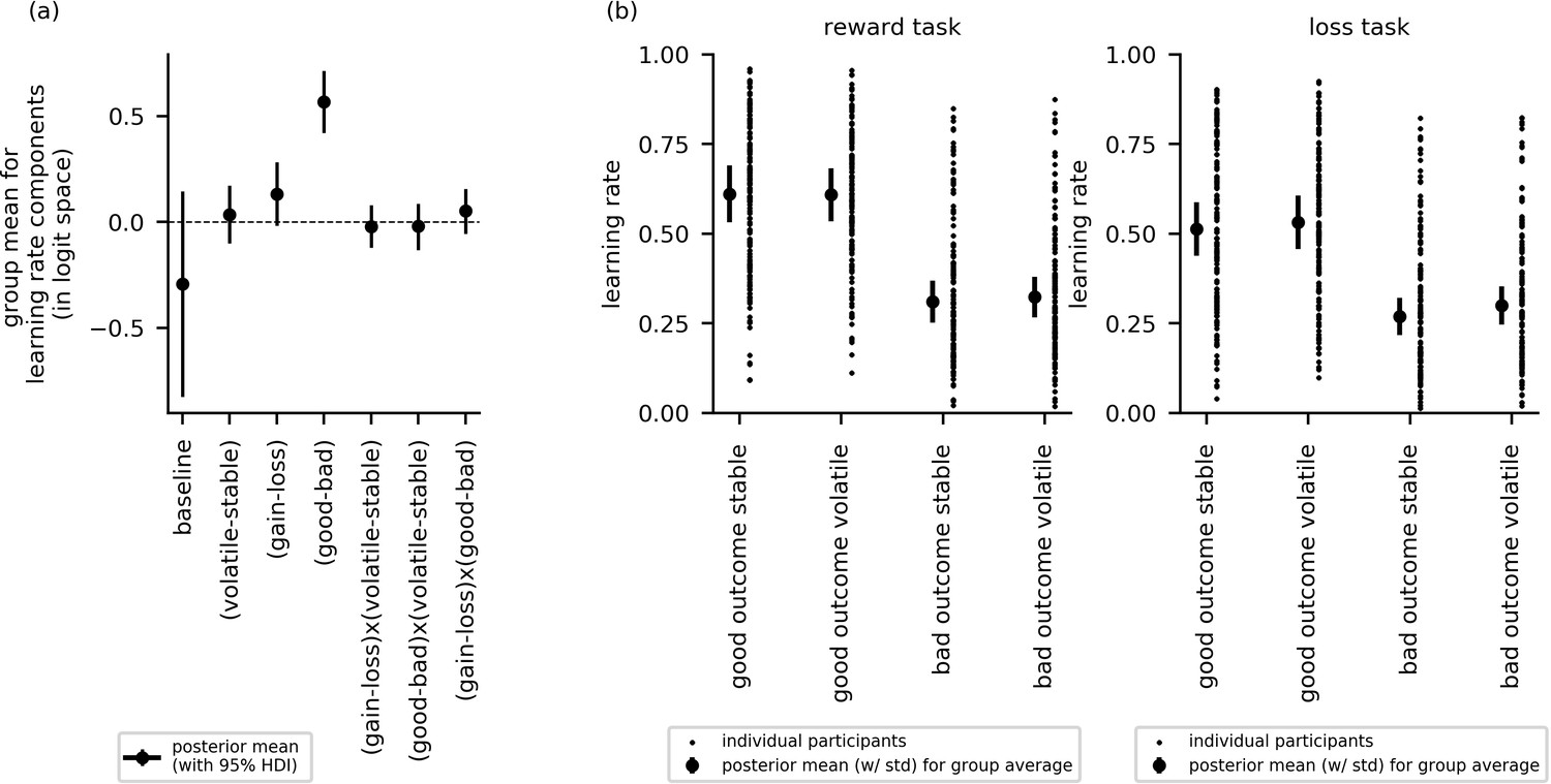
Cross-group results from experiment 2 for effects of block type (volatile, stable), task version (reward, aversive), and relative outcome value (good, bad) on learning rate.
(a) This panel shows the posterior means along with the 95% highest posterior density intervals (HDI) for the group means () for each learning rate component (i.e. for baseline learning rate and the change in learning rate as a function of each factor and their two-way interactions). The 95% posterior interval excluded zero for effect of relative outcome value (good - bad) upon learning rate. In contrast to experiment 1, there was no credible effect of block type upon learning rate () or of task version (). None of the two-way interactions were credible. (b) In this panel, the learning rate components are combined to illustrate how learning rates changed across conditions. The posterior mean learning rate for individual participants (small dots) and the group posterior mean learning rate (large dots, error bars represent the associated posterior standard deviation) are given for each of the eight conditions; these values were calculated from the posterior distributions of the learning rate components ( etc.) and the group means ().
Figure 5—figure supplement 2
Effect of depression-specific and anxiety-specific factors on learning rate and its components (data from experiment 2).
Panel (a) and panel (b) show the effects of depression-specific factor scores and anxiety-specific factor scores, respectively, on each of the learning rate components (e.g. ). The 95%-HDI’s for population-level parameters and included zero for all parameter components. This indicates that, as observed in experiment 1, neither depression-specific nor anxiety-specific factor scores credibly modulated learning rate as a function of block type (volatile versus stable), task version (reward versus aversive), or relative outcome value (good versus bad), or as a function of any of the two-way interactions of these experimental factors.
Appendix 4—figure 1
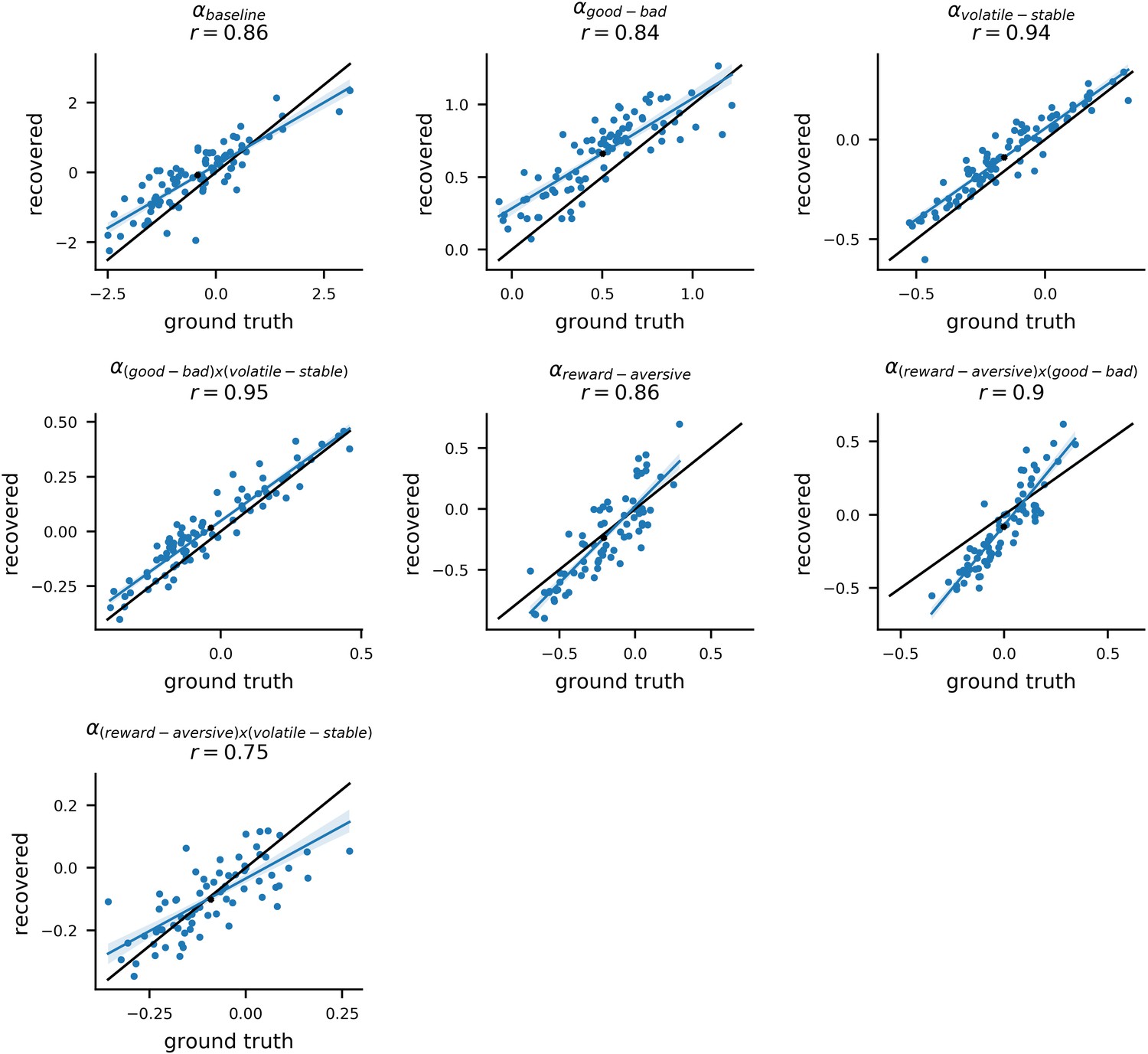
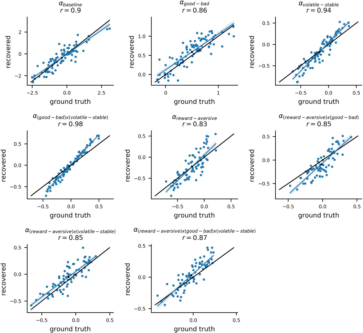
Recovery of individual-level learning rate parameters.
Posterior mean parameter estimates for participants from experiment 1 were used to simulate new choice data from the winning model (#11). The model was then re-fit to each of these simulated datasets. The original parameters estimated from the actual dataset (referred to as ‘ground truth’ parameters) were correlated with the newly estimated parameters (referred to as ‘recovered’ parameters) for each simulated dataset. An example dataset is shown here. Each panel shows the ground truth and recovered posterior means for a separate component of the composite learning rate parameter. The x-axis corresponds to original ‘ground truth’ parameter values and the y-axis corresponds to the recovered parameter values; each datapoint represents an individual participant. The average correlation between ground truth and recovered parameters values for learning rate components, across 10 simulated datasets, was r = 0.88 (std = 0.13).
Appendix 4—figure 2

Recovery of other model parameters.
Posterior mean parameter estimates for participants from experiment 1 were used to simulate new choice data from the winning model (#11). As in Appendix 4—figure 1, we show the results of parameter recovery for one example simulated dataset; here, we present data for parameters other than learning rate. Each panel shows the ground truth and recovered posterior means for a separate model parameter component. The x-axis corresponds to original ‘ground truth’ parameter values and the y-axis corresponds to the recovered parameter values; each datapoint represents an individual participant. The average correlation between ground truth and recovered parameters values across the 10 datasets for other (non-learning rate) parameters was r = 0.76 (std = 0.15).
Appendix 4—figure 3
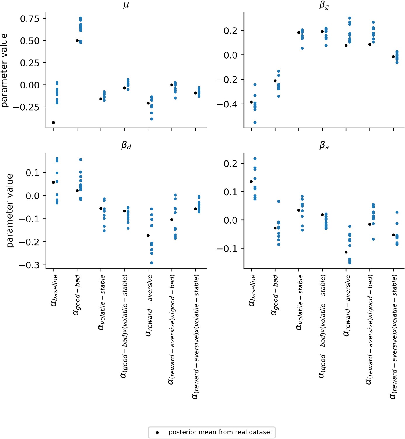
Variability of population-level learning rate parameters across simulated datasets.
The robustness of the estimates for the population-level parameters () was explored by examining the variability in parameter values across the 10 simulated datasets (blue data points). Population-level parameters corresponding to learning rate components are shown in this figure. The simulated datasets used for this analysis were the same as those used for Appendix 4—figure 1 and Appendix 4—figure 2. Since each of the 10 simulated datasets uses the same ground-truth parameters for generating data (black data points), differences across these datasets reflect an estimate for the amount of noise in participants’ choices; this choice noisiness is captured by the two inverse temperatures in the model. Consistency across datasets and proximity to the ground-truth parameters indicates a robustness to this type of noise.
Appendix 4—figure 4
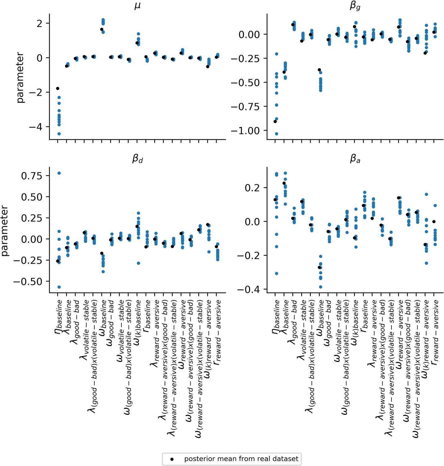
Variability of population-level parameters across simulated datasets for other parameters.
The robustness of the estimates for the population-level parameters () was explored by examining the variability in parameter values across the 10 simulated datasets (blue data points). Population-level parameters corresponding to all other parameter components aside from those for learning rate are shown in this figure. The simulated datasets used for this analysis were the same as those used for Appendix 4—figure 1 and Appendix 4—figure 2. Since each of the 10 simulated datasets uses the same ground-truth parameters for generating data (black data points), differences across these datasets reflect an estimate for the amount of noise in participants’ choices; this choice noisiness is captured by the two inverse temperatures in the model. Consistency across datasets and proximity to the ground-truth parameters indicates a robustness to this type of noise. Apart from the baseline component of each parameter, simulated parameter component ranges are relatively narrow and predominantly encompass the parameter values estimated from the actual dataset (black data points).
Appendix 4—figure 5
Recovery of individual-level learning rate parameters in the thee-way interaction model.
In experiment 1, we additionally fit a model that included the three-way interaction of block type (volatile, stable), relative outcome value (good, bad), and task version (reward, aversive) for learning rate. This model was identical to the winning model (#11) except for the inclusion of the three-way interaction and was used to confirm that the relationship between general factor scores and the interaction of block type by relative outcome value on learning rate did not vary as a function of task version. Posterior means for each participants’ model parameters were used to simulate new choice data from the model. The model was then re-fit to each of these simulated datasets. The original parameters estimated from the actual dataset (referred to as ‘ground truth’ parameters) were correlated with the newly estimated parameters (referred to as ‘recovered’ parameters) for each simulated dataset. An example dataset is shown here. Each panel shows the ground truth and recovered posterior means for a separate component of the composite learning rate parameter. The x-axis corresponds to original ground truth parameter values and the y-axis corresponds to the recovered parameter values; each datapoint represents an individual participant. The high correlation between the ground truth and recovered parameters was high, even for the triple interaction (bottom right panel), indicating good parameter recoverability. The average correlation between ground truth and recovered parameters values for this triple interaction, across 10 simulated datasets, was r = 0.86 (std = 0.10).
Appendix 5—figure 1
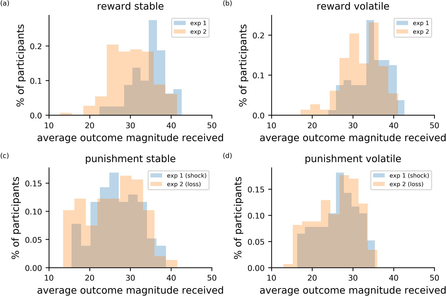
Comparison of task performance between experiment 1 and experiment 2.
The four panels depict the performance of participants in each block (stable left column; volatile right column) and in each task (reward top row; punishment bottom row). Data from experiment 1 is shown in blue; data from experiment 2 is shown in orange. To assess performance, the magnitudes of outcomes received were averaged across trials. Higher average magnitudes for the reward condition indicates better performance. Higher average magnitudes for the loss and shock outcomes indicates worse performance.
Appendix 6—figure 1
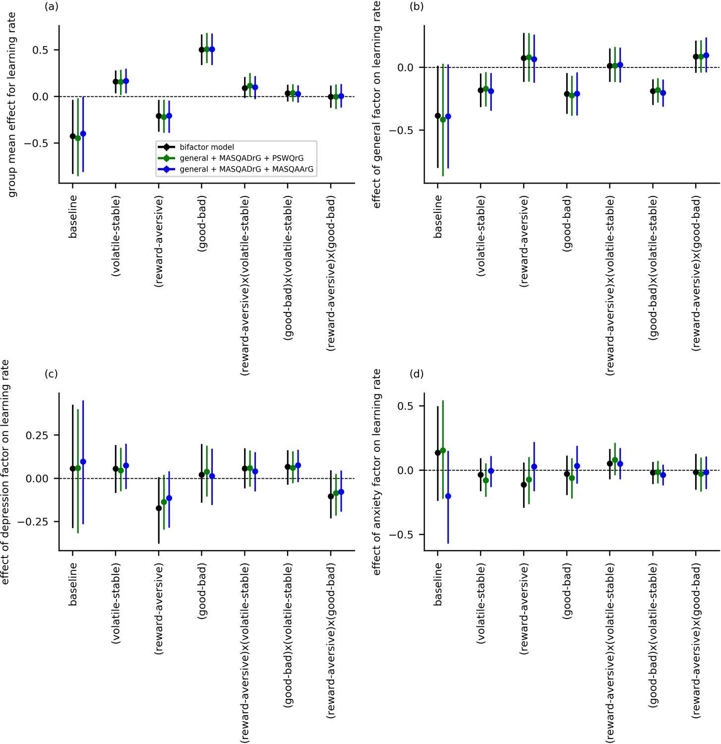
Learning rate parameters for experiment 1 data as estimated using alternate population-level parameters for specific effects of anxiety and depression.
Two alternative models were fit to the behavioral data from experiment 1, in addition to the main bifactor model. For the first alternative model, population-level parameters entered comprised scores on the general factor and residual scores on the MASQ anhedonia subscale and the Penn-State Worry Questionnaire (PSWQ). These residual scores were created by removing variance from scores for the MASQ and PSWQ explainable by scores for the general factor; as such these scores provide alternative depression-specific and anxiety-specific symptom measures. This model is abbreviated as ‘general + MASQADrG + PSWQrG’. For the second alternative model, residual PSWQ scores were replaced by residual scores for the MASQ anxious arousal subscale. This enables us to investigate whether anxiety-related symptoms uniquely captured by the MASQ-AA influence learning rate. This model is abbreviated as ‘general + MASQADrG + MASQAArG’. The main model is labeled simply as ‘bifactor model’. Both alternative models yielded general factor learning rate effects that were consistent with the main model (panel b). No additional effects were observed for the depression or anxiety subscales (panels c-d).
Appendix 6—figure 2
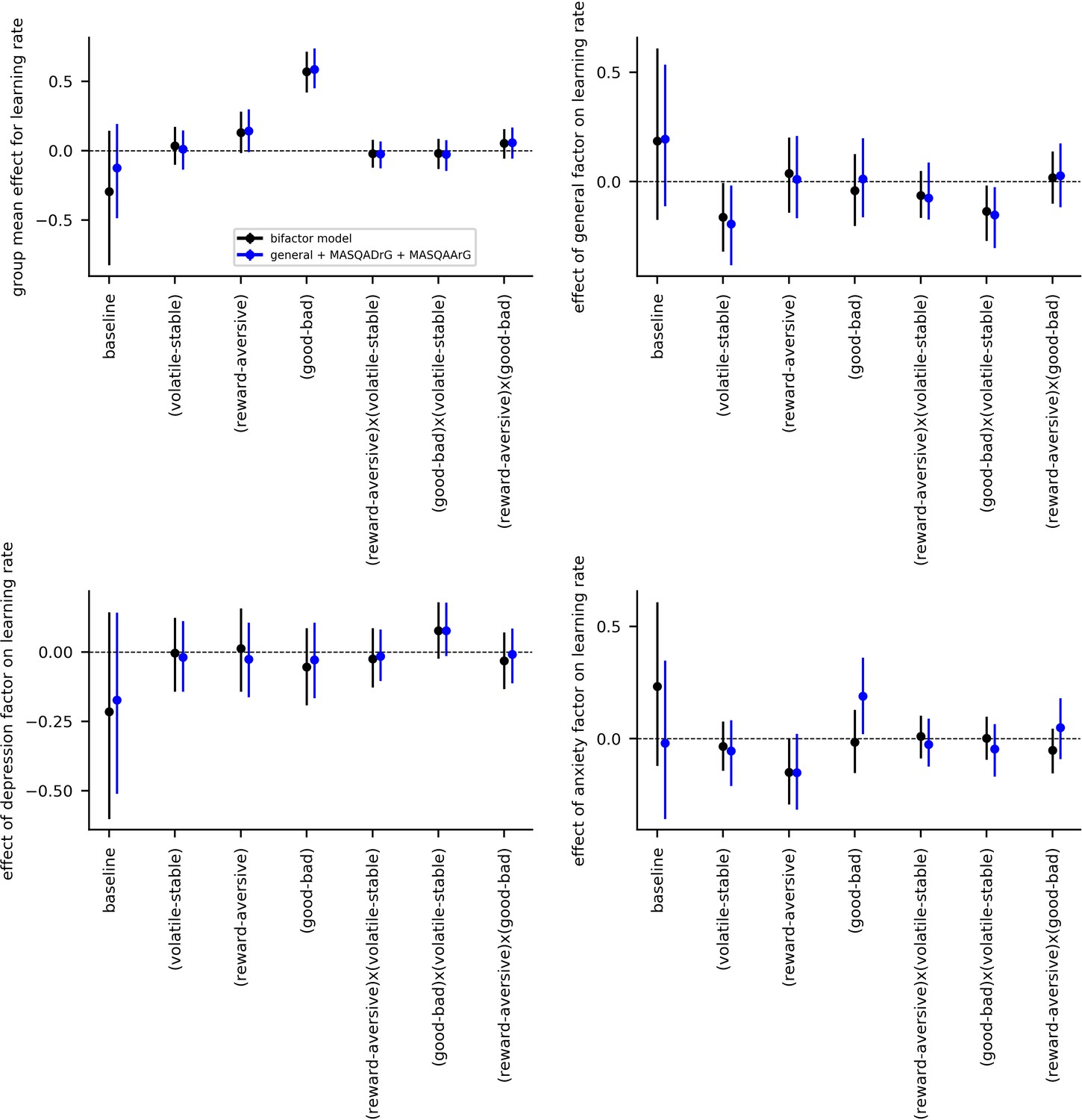
Learning rate parameters for experiment 2 data as estimated using alternate population-level parameters for specific effects of anxiety and depression.
In addition to the main bifactor model, an additional alternative model was also fit to the behavioral data from experiment 2. In this model (the second alternate model described in Appendix 6—figure 1), population-level parameters entered comprised scores on the general factor and residual scores on the MASQ anhedonia subscale and the MASQ anxious arousal subscale (having regressed out variance explainable by general factor scores). This model is abbreviated as ‘general + MASQADrG + MASQAArG’. As in Appendix 6—figure 1, the main model is labeled simply as ‘bifactor model’. The alternative model yielded general factor learning rate effects that were consistent with the main model (panel b). No additional effects were observed for residual scores on the MASQ-AD subscale (panel c). Elevated residual scores on the MASQ-AA subscale were linked to increased learning after outcomes of relative positive value (good - bad) but did not modulate adaptation of learning rate to volatility or the interaction of volatility and relative outcome value (good - bad). We note, no equivalent findings were observed for MASQ-AA in experiment 1 (see Appendix 6—figure 1). We could not fit the ‘general + MASQADrG + PSWQ’ model also described in Appendix 6—figure 1 to this dataset as participants were not administered the PSWQ questionnaire.
Appendix 7—figure 1
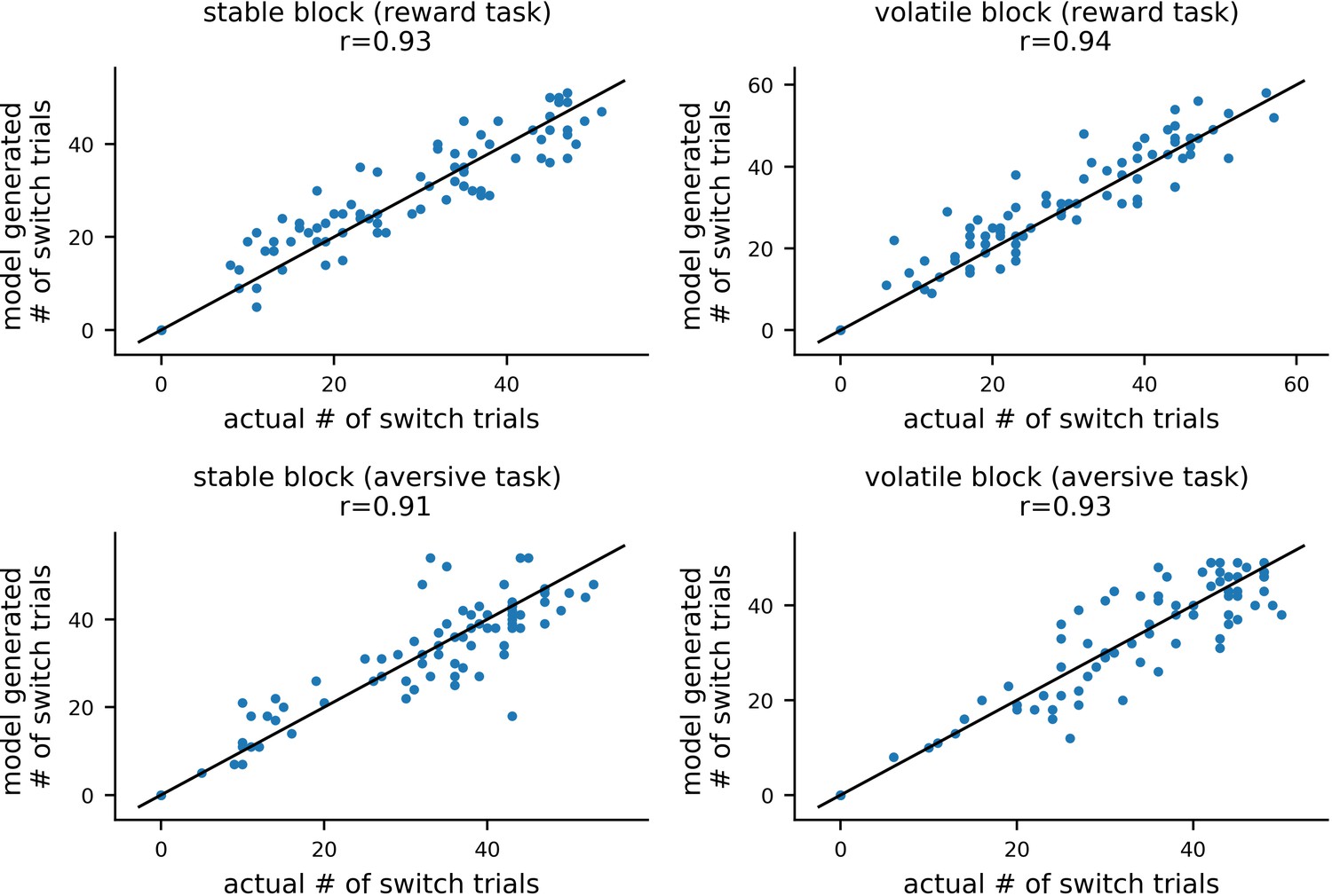
Comparison of actual and model generated numbers of switch trials in experiment 1.
For each participant, we calculated the number of trials on which they switched choice of shape. As described under parameter recovery, each participant’s posterior means for each of model #11 parameters were used together with model #11 to simulate 10 new datasets. For each of these simulated datasets, the number of switch trials was computed and correlated with the actual number of switch trial for the corresponding participant. This is shown here for an example dataset, with switch trials for each combination of task version (reward, aversive) and block type (volatile, stable) shown in a separate panel. Mean correlations between actual and generated switch trials were high (rs >0.88 across the 4 conditions and 10 datasets), demonstrating that the model can reproduce a basic qualitative feature of participants’ choice behavior.
Appendix 7—figure 2

Comparison of actual and model generated numbers of switch trials in experiment 2.
For each participant, we calculated the number of trials on which they switched choice of shape. As described under parameter recovery, each participant’s posterior means for each of model #11 parameters were used together with model #11 to simulate 10 new datasets. For each of these simulated datasets, the number of switch trials was computed and correlated with the actual number of switch trial for the corresponding participant. This is shown here for an example dataset, with switch trials for each combination of task version (reward, aversive) and block type (volatile, stable) shown in a separate panel. Mean correlations between actual and generated switch trials were high (rs >0.80 across the 4 conditions and 10 datasets), demonstrating that the model can reproduce a basic qualitative feature of participants’ choice behavior.
Author response image 1
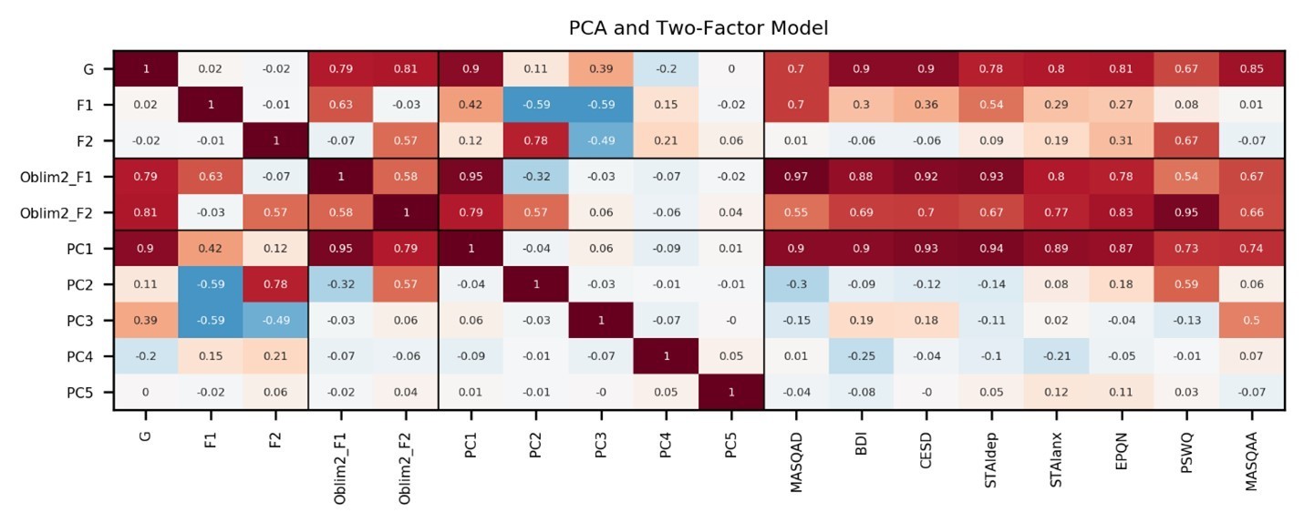
Information captured by top five PCs: We conducted PCA on the item-level questionnaire responses from experiment 1 (n=86).
Scores on the first PC correlated highly with general factor scores (r=0.9). Scores on the second PC correlated strongly positively with PSWQ (r=0.59), and moderately negatively with MASQAD (r=-0.3),. The third PC correlated most strongly with MASQAA (r=0.5), but also correlated moderately with the BDI and CESD (r=0.19, r=0.18). The fourth PC correlated moderately with BDI (r=-0.25) but not with CESD (r=-0.03), perhaps capturing something specific to the BDI. The fifth PC did not correlate strongly with any subscale. Correlations are shown for the experiment 1 dataset only, on which the PCA and correlated factors model were estimated.
Author response image 2
Tables
Appendix 1—table 1
Basic demographic details for participants in Experiment 1.
| Participant recruitment group | Major Depressive Disorder (MDD) | Generalized Anxiety Disorder (GAD) | Healthy Controls | Unselected Community Sample |
|---|---|---|---|---|
| Participants Total N (N for reward task, N for aversive task) | 20 (19, 17) | 12 (10, 11) | 24 (22, 19) | 30 (29, 30) |
| Female | 10 (10, 8) | 11 (9, 10) | 16 (14, 13) | 13 (12, 13) |
| Age mean ± sd (for reward task, for aversive task) | 31 ± 10 (31 ± 10, 28 ± 10) | 32 ± 9 (31 ± 9, 32 ± 9) | 27 ± 6 (27 ± 6, 28 ± 6) | 27 ± 5 (27 ± 5, 27 ± 5) |
| STAI mean ± sd (for reward task, for aversive task) | 59 ± 6 (59 ± 7, 58 ± 6) | 58 ± 9 (60 ± 9, 57 ± 9) | 40 ± 12 (41 ± 12, 41 ± 12) | 36 ± 12 (36 ± 11, 36 ± 12) |
| BDI mean ± sd (for reward task, for aversive task) | 24 ± 9 (25 ± 9, 23 ± 9) | 20 ± 11 (22 ± 10, 20 ± 11) | 7 ± 7 (7 ± 7, 7 ± 8) | 6 ± 8 (5 ± 7, 6 ± 8) |
| MASQ-AD mean ± sd (for reward task, for aversive task) | 80 ± 10 (81 ± 10, 79 ± 10) | 74 ± 16 (75 ± 17, 73 ± 16) | 55 ± 18 (56 ± 18, 56 ± 19) | 50 ± 20 (48 ± 18, 50 ± 20) |
| MASQ-AA mean ± sd (for reward task, for aversive task) | 28 ± 7 (28 ± 7, 28 ± 7) | 33 ± 10 (34 ± 11, 34 ± 10) | 21 ± 4 (21 ± 4, 20 ± 2) | 22 ± 6 (22 ± 6, 22 ± 6) |
| PSWQ mean ± sd (for reward task, for aversive task) | 62 ± 14 (61 ± 14, 60 ± 14) | 76 ± 9 (75 ± 9, 75 ± 9) | 52 ± 13 (54 ± 12, 51 ± 14) | 42 ± 15 (42 ± 15, 42 ± 15) |
| CESD mean ± sd (for reward task, for aversive task) | 30 ± 9 (30 ± 9, 28 ± 8) | 30 ± 14 (32 ± 14, 30 ± 14) | 12 ± 8 (12 ± 8, 11 ± 8) | 10 ± 11 (9 ± 10, 10 ± 11) |
| EPQ-N mean ± sd (for reward task, for aversive task) | 18 ± 3 (18 ± 3, 17 ± 3) | 19 ± 4 (19 ± 3, 18 ± 4) | 10 ± 6 (11 ± 6, 10 ± 6) | 10 ± 6 (10 ± 6, 10 ± 6) |
| General Factor mean ± sd (for reward task, for aversive task) | 1.1 ± 0.8 (1.1 ± 0.9, 1.0 ± 0.8) | 1.3 ± 1.0 (1.5 ± 1.0, 1.4 ± 1.0) | −0.3 ± 0.8 (−0.2 ± 0.8,–0.4 ± 0.7) | −0.2 ± 0.8 (−0.3 ± 0.7,–0.2 ± 0.8) |
| Depression-Specific Factor mean ± sd (for reward task, for aversive task) | 0.8 ± 1.0 (0.9 ± 1.0, 0.8 ± 1.1) | −0.0 ± 0.8 (−0.1 ± 0.8,–0.1 ± 0.7) | 0.1 ± 1.2 (0.1 ± 1.2, 0.3 ± 1.2) | −0.2 ± 0.9 (−0.2 ± 0.9,–0.2 ± 0.9) |
| Anxiety-Specific Factor mean ± sd (for reward task, for aversive task) | −0.5 ± 1.1 (−0.5 ± 1.1,–0.6 ± 1.2) | 0.8 ± 0.9 (0.5 ± 0.8, 0.7 ± 0.9) | −0.2 ± 0.9 (−0.1 ± 0.8,–0.1 ± 0.9) | −0.3 ± 1.1 (−0.3 ± 1.1,–0.3 ± 1.1) |
-
STAI = Spielberger State-Trait Anxiety Inventory (form Y; Spielberger et al., 1983) BDI = Beck Depression Inventory (Beck et al., 1961) MASQ-AD/MASQ AA=anhedonic depression and anxious arousal subscales for the Mood and Anxiety Symptoms Questionnaire (Clark and Watson, 1995; Watson and Clark, 1991) PSWQ = Penn State Worry Questionnaire (Meyer et al., 1990) CESD = Center for Epidemiologic Studies Depression Scale (Radloff, 1977) EPQ-N = the Neuroticism subscale for the 80-item Eysenck Personality Questionnaire (Eysenck and Eysenck, 1975). The two healthy control participants whose data were excluded from both tasks are omitted from this table.
Appendix 1—table 2
Basic demographic details of participants who provided questionnaire data for the confirmatory factor analysis.
| Number of participants (Total N) | 199 |
|---|---|
| Female (N) | 120 |
| Age (mean ± sd) | 21 ± 4 |
| STAI (mean ± sd) | 44 ± 9 |
| BDI (mean ± sd) | 7 ± 6 |
| MASQ-AD (mean ± sd) | 54 ± 15 |
| MASQ-AA (mean ± sd) | 24 ± 8 |
| PSWQ (mean ± sd) | 57 ± 13 |
| CESD (mean ± sd) | 24 ± 8 |
| EPQ-N (mean ± sd) | 6 ± 4 |
| General Factor (mean ± sd) | −0.1 ± 1.0 |
| Depression-Specific Factor (mean ± sd) | 0.4 ± 1.0 |
| Anxiety-Specific Factor (mean ± sd) | −0.1 ± 1.0 |
-
STAI = Spielberger State-Trait Anxiety Inventory (form Y; Spielberger et al., 1983) BDI = Beck Depression Inventory (Beck et al., 1961) MASQ-AD/MASQ AA=anhedonic depression and anxious arousal subscales for the Mood and Anxiety Symptoms Questionnaire (Clark and Watson, 1995; Watson and Clark, 1991) PSWQ = Penn State Worry Questionnaire (Meyer et al., 1990) CESD = Center for Epidemiologic Studies Depression Scale (Radloff, 1977) EPQ-N = the Neuroticism subscale for the 80-item Eysenck Personality Questionnaire (Eysenck and Eysenck, 1975).
Appendix 1—table 3
Basic demographic details for participants in Experiment 2.
| Participants (Total N) | 147 |
|---|---|
| Female (N) | 64 |
| Age | Not recorded; required to be 18 years or older. |
| STAI (mean ± sd) | 43 ± 13 |
| BDI (mean ± sd) | 11 ± 12 |
| MASQ-AD (mean ± sd) | 63 ± 18 |
| MASQ-AA (mean ± sd) | 23 ± 8 |
| General Factor (mean ± sd) | −0.1 ± 0.9 |
| Depression-Specific Factor (mean ± sd) | −0.2 ± 0.9 |
| Anxiety-Specific Factor (mean ± sd) | 0.1 ± 1.0 |
-
STAI = Spielberger State-Trait Anxiety Inventory (form Y; Spielberger et al., 1983); BDI = Beck Depression Inventory (Beck et al., 1961) MASQ-AD/MASQ AA=anhedonic depression and anxious arousal subscales for the Mood and Anxiety Symptoms Questionnaire (Clark and Watson, 1995; Watson and Clark, 1991).
Appendix 3—table 1
Model comparison table for Experiment 1.
Thirteen models were fit to participants’ choice data from experiment 1. Models were fit hierarchically and compared using leave-one-out cross validation error approximated by Pareto smoothed importance sampling (PSIS-LOO; values shown in right-most column). The model with the lowest PSIS-LOO was selected as the winning model and used to make inferences about the relationships between task performance and internalizing symptoms.
| Model Number | Parameters | # of Parameter Components | PSIS-LOO |
|---|---|---|---|
| Model #1 | 12 | 27,801 | |
| Model #2 | 12 | 26,164 | |
| Model #3 | 15 | 25,550 | |
| Model #4 | 18 | 26,042 | |
| Model #5 | 21 | 25,462 | |
| Model #6 | 24 | 25,486 | |
| Model #7 | 23 | 25,154 | |
| Model #8 | 25 | 25,185 | |
| Model #9 | 27 | 25,377 | |
| Model #10 | 27 | 25,325 | |
| Model #11 ** | 26 | 25,037 | |
| Model #12 | 32 | 25,216 | |
| Model #13 | 32 | 25,181 |
-
1:Unless otherwise stated, each parameter is divided into four parameter components: a shared baseline parameter across blocks and tasks, and differences in the parameter between stable and volatile blocks (volatile-stable), between different task versions (reward-aversive) and an interaction of those differences (reward-aversive)x(volatile-stable).
gb: For each parameter with this superscript, three additional parameter components were added for the relative value of previous outcome (good-bad) and the interactions of relative outcome value with block type (volatile-stable)x(good-bad) and task version (reward-aversive)x(good-bad).
-
ra only: For each parameter with this superscript, only differences in the parameters between the reward and aversive task versions (reward-aversive) were included.
baseline: For each parameter with this superscript, only one single baseline parameter was used, across both task versions and volatile and stable blocks.
-
**Indicates best fitting model.
Appendix 3—table 2
Model comparison table for Experiment 2.
The same 13 models fit to participants’ choice data from experiment 1 were also fit to participants’ choice data from experiment 2. Models were fit hierarchically and compared using leave-one-out cross validation error approximated by Pareto smoothed importance sampling (PSIS-LOO). Model #12 (which differs from model #11 only in the use of separate learning rates for each shape) had a slightly lower PSIS-LOO than model #11. However, the difference in PSIS-LOO for Models #11 and #12 was within one standard error (difference in PSIS-LOO = 43; SE = 49). In contrast, model #11’s PSIS-LOO was more than two standard errors better than model #12 in experiment 1 (difference in PSIS-LOO = 179, SE = 71). Hence, if we seek to retain one model across both experiments, model #11 is the better choice.
| Model Number | Parameters | # of Parameter Components | PSIS-LOO |
|---|---|---|---|
| Model #1 | 1 | 12 | 57,520 |
| Model #2 | 12 | 54,002 | |
| Model #3 | 15 | 52,918 | |
| Model #4 | 18 | 53,755 | |
| Model #5 | 21 | 52,758 | |
| Model #6 | 24 | 52,769 | |
| Model #7 | 23 | 52,139 | |
| Model #8 | 25 | 52,136 | |
| Model #9 | 27 | 52,083 | |
| Model #10 | 27 | 52,169 | |
| Model #11 | 26 | 52,048 | |
| Model #12 | 32 | 52,005 | |
| Model #13 | 32 | 52,084 |
-
1:Unless otherwise stated, each parameter is divided into four parameter components: a shared baseline parameter across blocks and tasks, and differences in the parameter between stable and volatile blocks (volatile-stable), between different task versions (gain-loss) and an interaction of those differences (gain-loss)x(volatile-stable).
gb: For each parameter with this superscript, three additional parameter components were added for the relative value of previous outcome (good-bad) and the interactions of this difference with block type (volatile-stable)x(good-bad), and task version (gain-loss)x(good-bad). gl only: For each parameter with this superscript, only differences in the parameters between the reward gain and reward loss task versions (gain-loss) were included.
-
baseline: For each parameter with this superscript, only one single baseline parameter was used, across both task versions and volatile and stable blocks.
Additional files
Download links
A two-part list of links to download the article, or parts of the article, in various formats.
Downloads (link to download the article as PDF)
Open citations (links to open the citations from this article in various online reference manager services)
Cite this article (links to download the citations from this article in formats compatible with various reference manager tools)
Impaired adaptation of learning to contingency volatility in internalizing psychopathology
eLife 9:e61387.
https://doi.org/10.7554/eLife.61387


