Demographic history mediates the effect of stratification on polygenic scores
- Department of Genetics, Perelman School of Medicine, University of Pennsylvania, United States
Figures
Figure 1 with 2 supplements
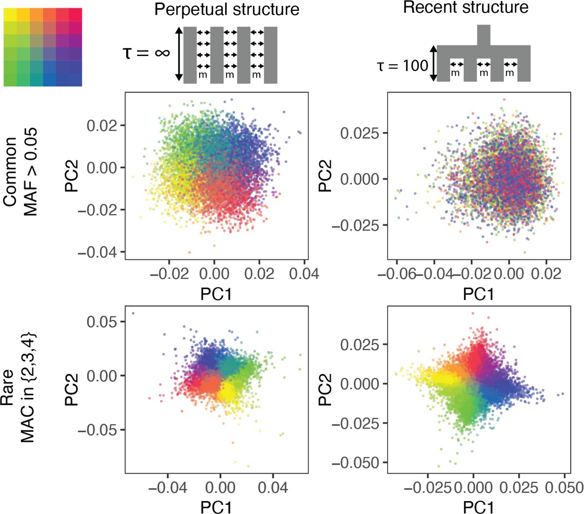
The ability of PCA to capture population structure depends on the frequency of the variants used and the demographic history of the sample.
Panels show the first and second principal components (PCs) of the genetic relationship matrix constructed from either common (upper row) or rare (lower row) variants. Each point is an individual (N = 9,000) and their color represents the deme in the grid (upper left) from which they were sampled. Both common (minor allele frequency >0.05) and rare (minor allele count = 2, 3, or 4) variants can be informative when population structure is ancient (left column; represents the time in generations in the past at which structure disappears) but only rare variants are informative about recent population structure (right column; generations). Number of variants used for PCA: 200,000 (upper row), 1 million (lower left), and ≈750,000 (lower right).
Figure 1—figure supplement 1
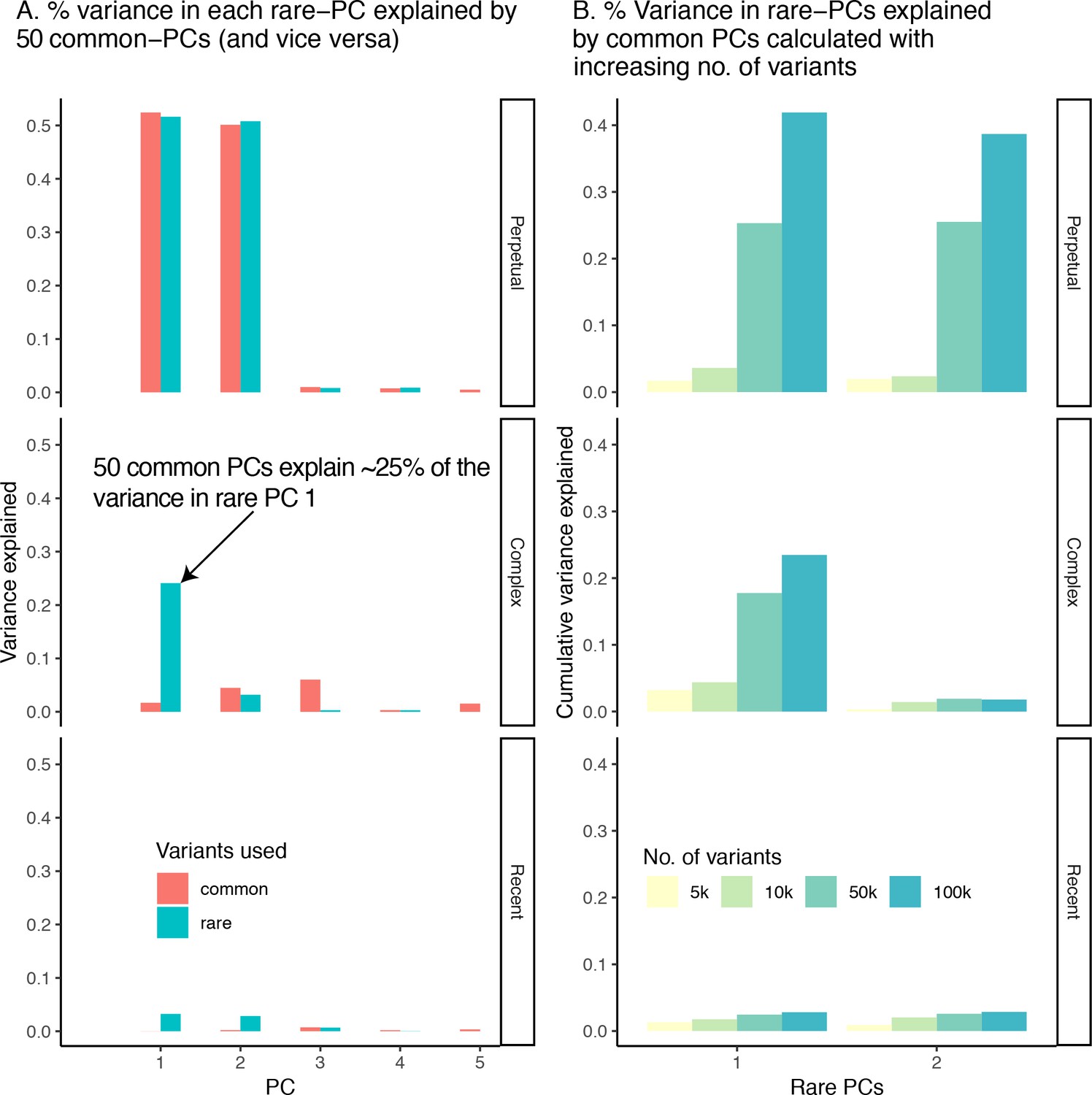
Collinearity between common- and rare-PCs under different demographic models.
(A) Proportion of variance in the first five rare-PCs (green) explained by 50 common-PCs (and vice versa). (B) Proportion of variance in rare-PC 1 and 2 explained by 50 common-PCs calculated using increasing number of common variants.
Figure 1—figure supplement 2
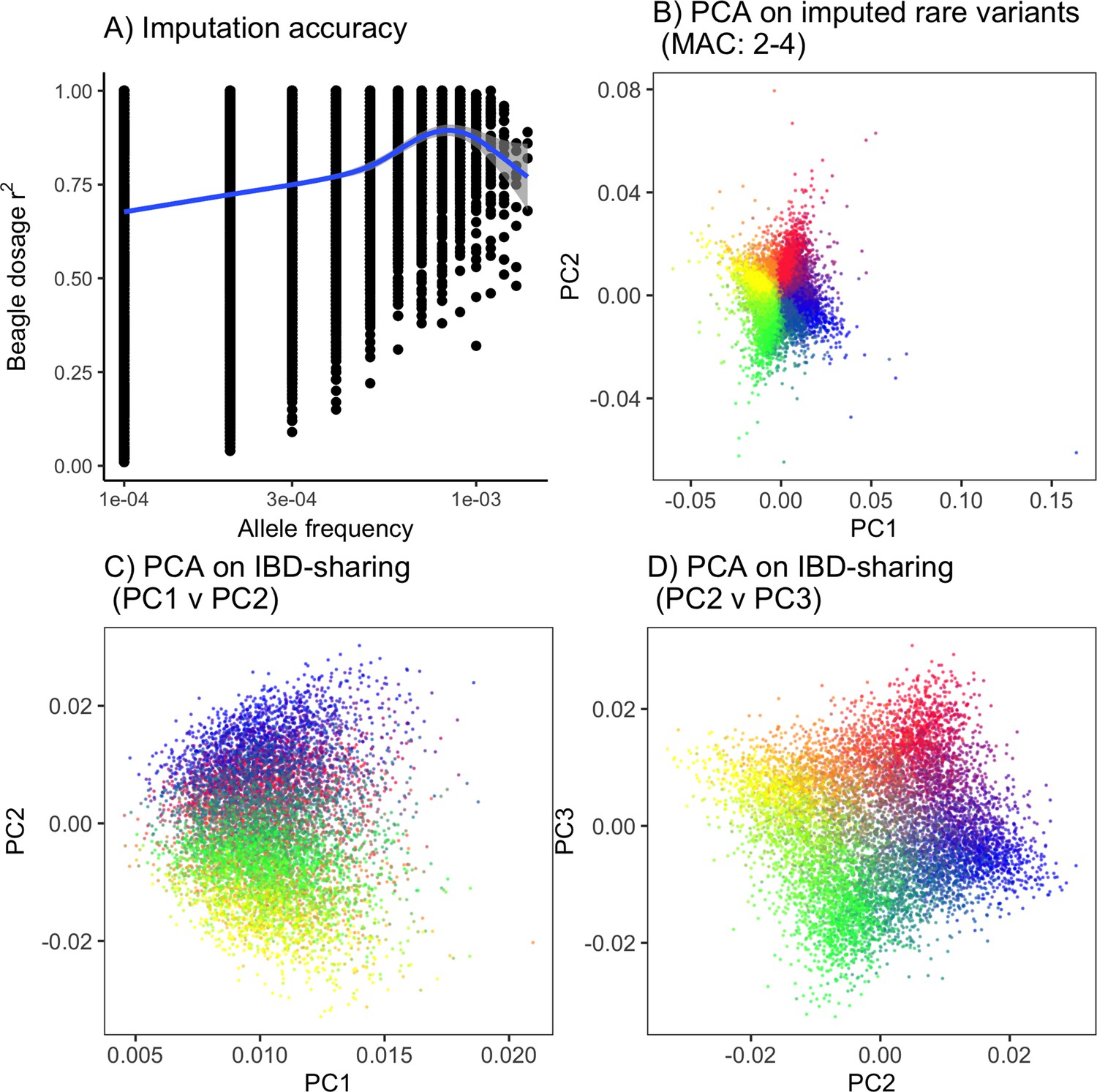
PCA on imputed rare variants and IBD-sharing provide an alternative to rare-PCA when sequence data are not available.
(A) Imputation accuracy as a function of frequency on a single chromosome. Even though imputation accuracy for rare variants is lower than that for common variants, (B) imputed rare variants still capture population structure in the ‘recent structure’ model. Alternatively, (C,D) PCA on IBD-sharing can be used to capture recent population structure.
Figure 2 with 1 supplement
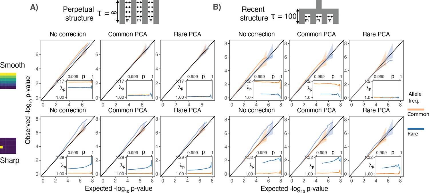
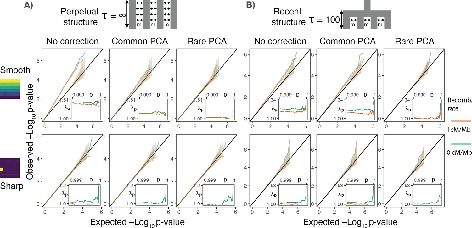
Test statistic inflation under two different demographic histories.
(A) Perpetual structure and (B) recent structure. Upper and lower rows show results for smoothly and sharply distributed environmental risk, respectively, whereas columns show different methods of correction. The simulated phenotype has no genetic contribution so any deviation from the diagonal represents inflation in the test statistic. Each panel shows QQ plots for -log10 p-value for common (orange) and rare (blue) variants. Insets show inflation () in the tail (99.9th percentile) of the distribution. Results are averaged across 20 simulations of the phenotype.
Figure 2—figure supplement 1
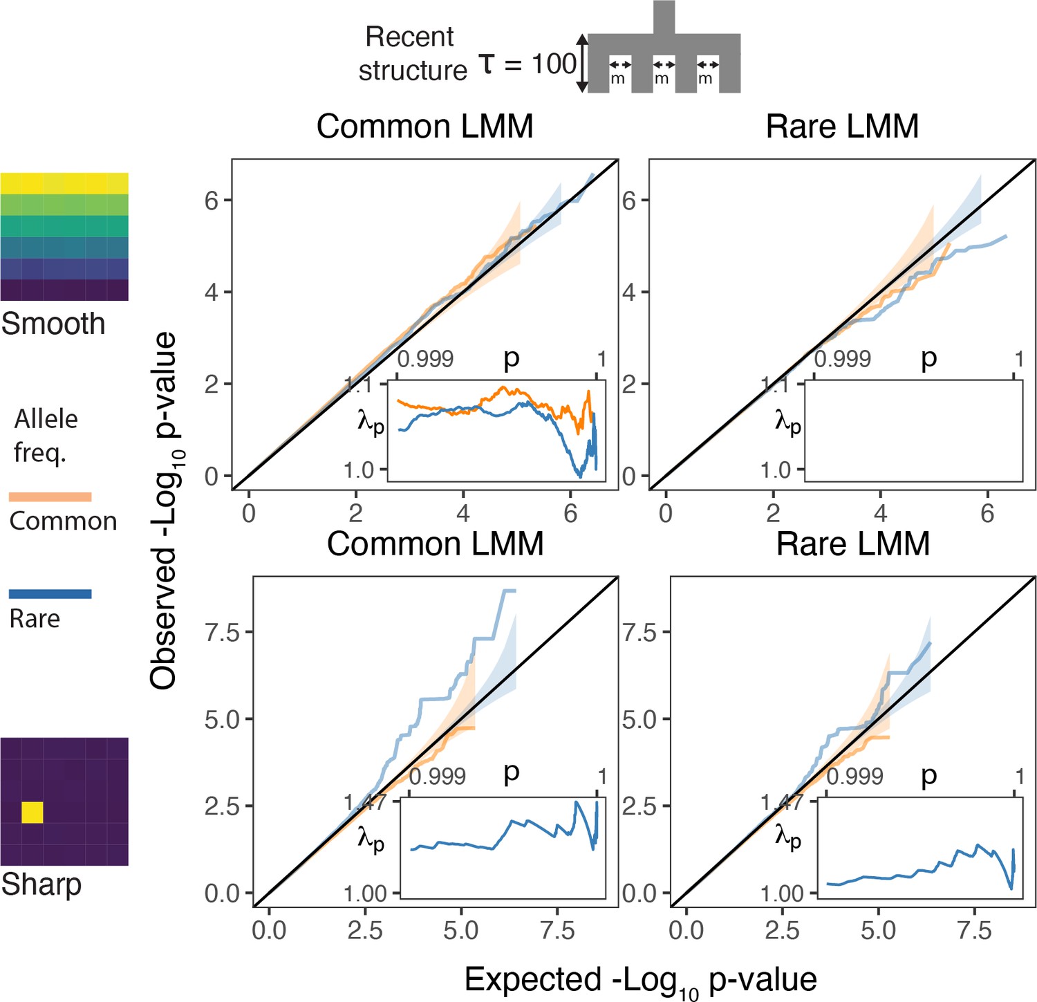
QQplots for linear mixed model association of non-heritable phenotypes carried out with GCTA-LOCO for genotypes generated under the recent structure model.
Models were fitted with either a genetic relatedness matrix constructed with common variants (left column) or with rare variants (right column). Insets show the 99.9% tail of the inflation factor. Orange and blue colored lines refer to common and rare variants, respectively. Results shown for a single simulation of the phenotype.
Figure 3 with 1 supplement
Gene burden tests are relatively robust to stratification.
QQ plots of expected and observed -log10p-value under the (A) perpetual and (B) recent structure models for the association of rare variant burden across a gene with total exon length of 1.3 kb (gene length of 7 kb) and non-heritable phenotype with a smooth (upper) or sharp (lower) distribution of environmental effects. Orange and green lines show results for a gene with and without recombination, respectively. Inset shows inflation in the tail (99.9%) of the test statistic distribution.
Figure 3—figure supplement 1
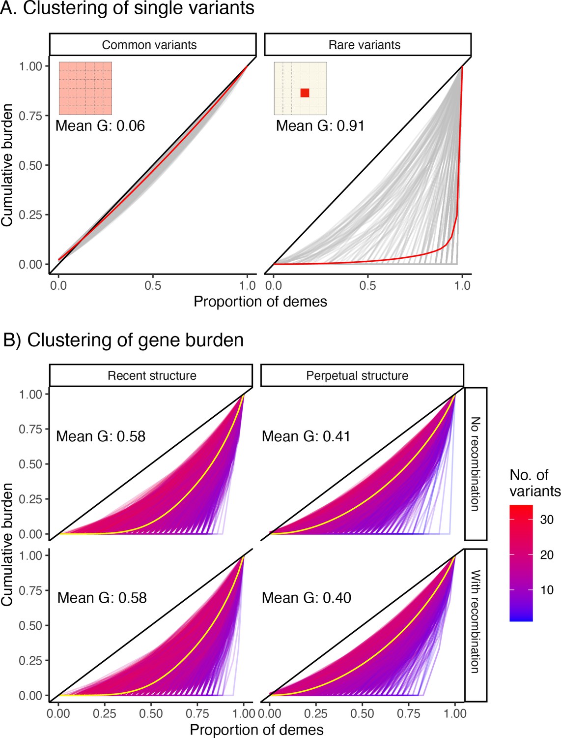
Gini curves showing geographic clustering of (A) variant frequency and (B) gene burden.
(A) Gray curves are individual variants (1,000 sampled uniformly at random for plotting), and red lines indicate the mean curve across all 1,000 variants. The diagonal represents the case where the variant/burden is uniformly distributed over the entire grid. Common variants tend to be more widely distributed (left panel) than rare variants (right) as illustrated by the grid inset. (B) Each curve represents a single gene (10,000 sampled), and the yellow line represents the mean across genes. The color of a curve represents the number of rare variants across which burden is aggregated. As the number of variants increases, gene burden behaves more like a common variant in its spatial distribution.
Figure 4 with 3 supplements
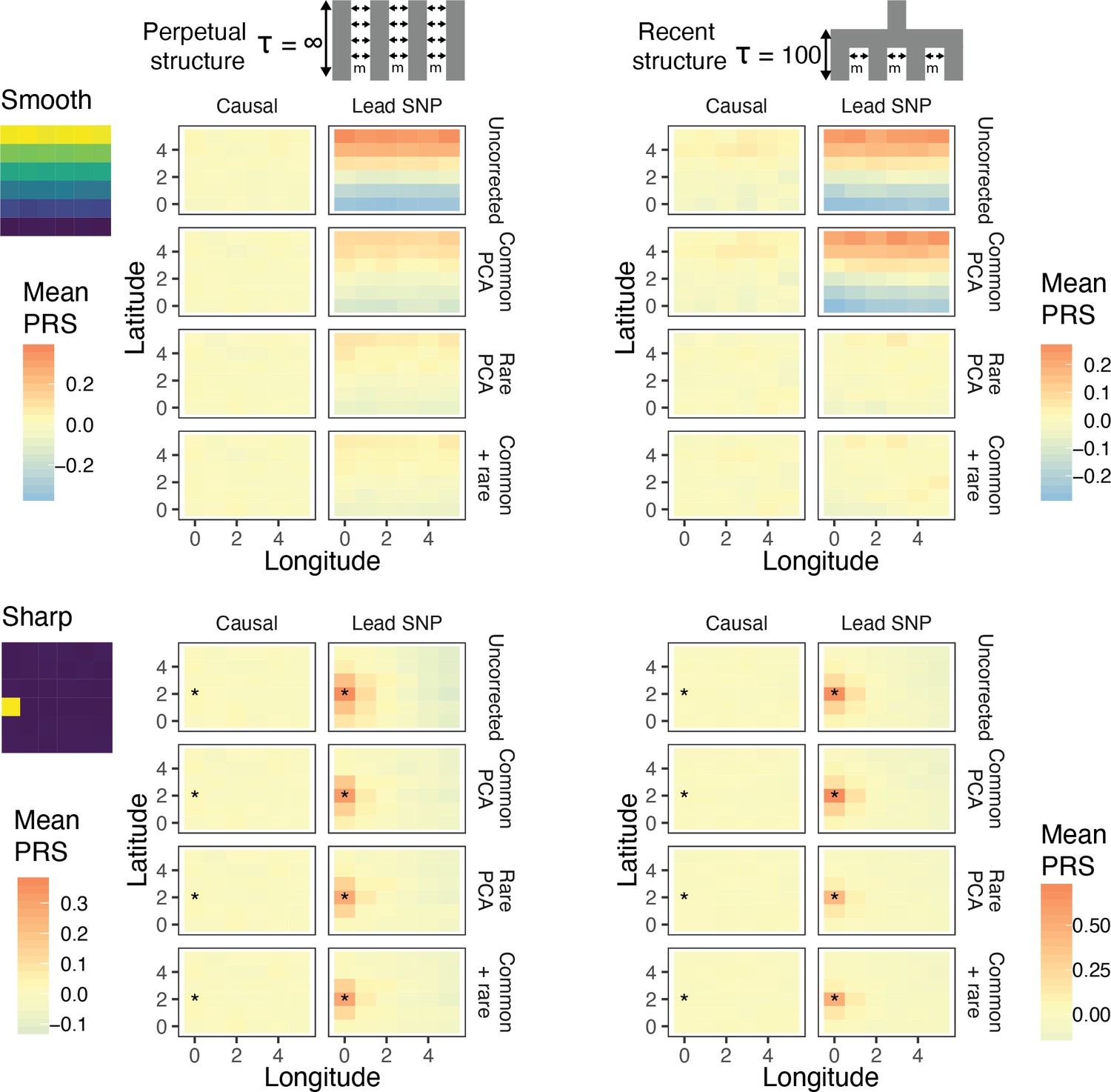
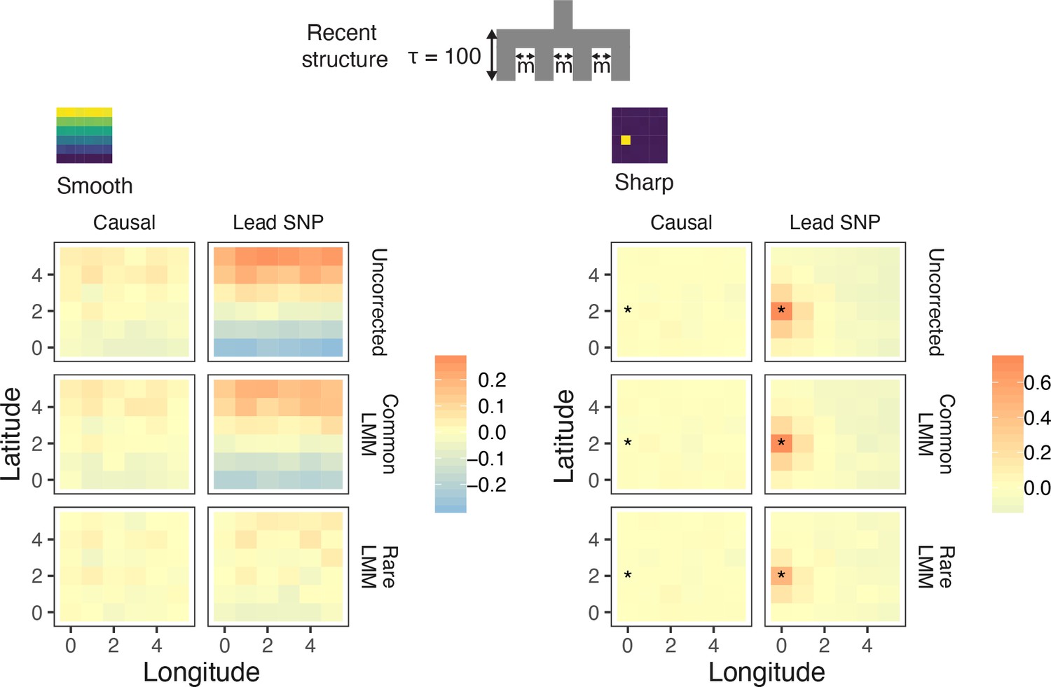
Residual stratification in effect size estimates translates to residual stratification in polygenic score in the (A) recent and (B) perpetual structure models.
The simulated phenotype in the training sample has a heritability of 0.8, distributed over 2,000 causal variants. Each small square is colored with the mean residual polygenic score for that deme in the test sample, averaged over 20 independent simulations of the phenotype. In each panel, the rows represent different methods of PCA correction and columns represent two different methods of variant ascertainment. ‘Causal’ refers to causal variants with p-value < 5×10⁻⁴, and ‘Lead SNP’ refers to a set of variants, where each represents the most significantly associated SNP with a p-value < 5×10⁻⁴ in a 100 kb window around the causal variant. The simulated environment is shown on the left. For the sharp effect, the affected deme is highlighted with an asterisk.
Figure 4—figure supplement 1
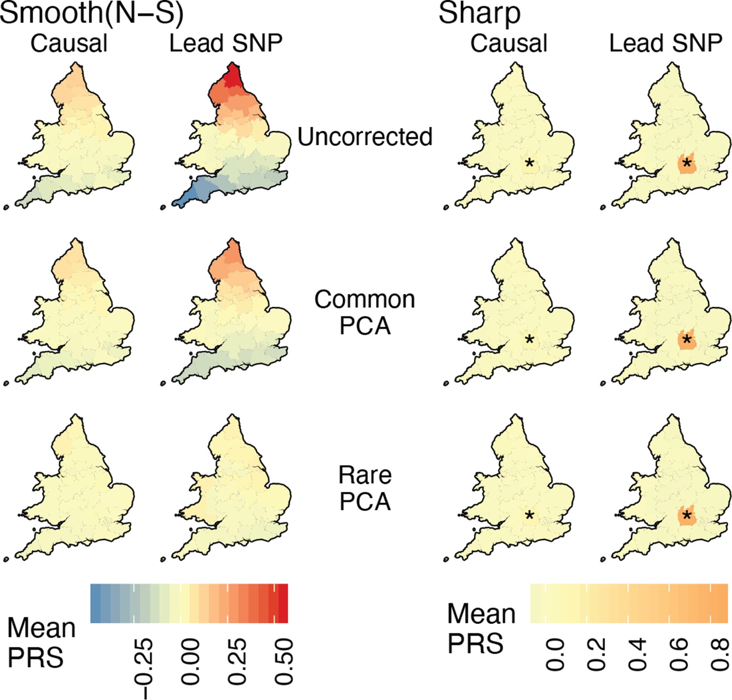
Spatial distribution of residual polygenic scores based on effect sizes from linear mixed models carried out in GCTA-LOCO.
Residual polygenic score in each deme was averaged across all individuals from that deme and over 10 simulations of the phenotype. The terms 'Causal' and 'Lead SNP' refer to polygenic scores constructed with known causal variants and topmost significant SNPs, respectively.
Figure 4—figure supplement 2
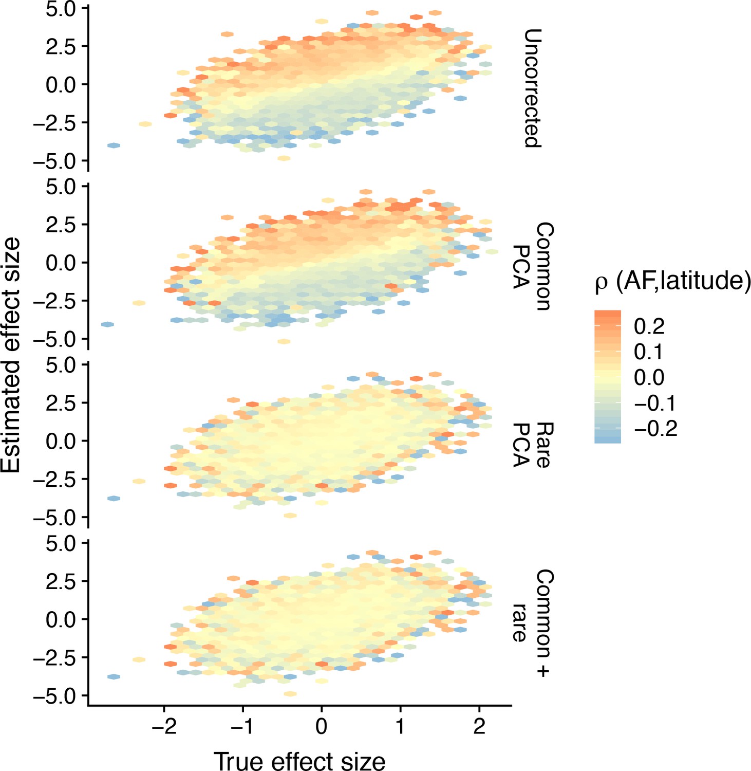
Hexagonal bin plots illustrating the residual confounding in variant effect sizes due to stratification.
Each panel shows the comparison of the true (simulated) and estimated effect sizes of causal variants (M = 2000) for different modes of correction for population structure and when the environment is smoothly distributed in a North-South cline. The color of each bin represents the mean correlation of variants in that bin and latitude, averaged across 20 simulations. When there is residual stratification, the effect sizes of variants that are positively correlated with latitude are biased upwards, whereas the effect sizes of variants that are negatively correlated are biased downwards. Even though the effect size of any single variant may be biased due to stratification, the effect size across all variants is still unbiased. In this particular case, because the population structure has a recent origin, rare-PCA, but not common-PCA adequately removes the bias.
Figure 4—figure supplement 3

Bias and prediction accuracy in polygenic scores as a function of variant ascertainment schemes.
Polygenic scores were calculated using (A) causal variants with p-value < 5e-04, (B) variants fine-mapped with SuSiE in windows where at least one variant has a p-value < 5e-04, and (C) the most significantly associated variants in windows where at least one variant has a p-value < 5e-04. Results presented here are based on the recent structure model. Bias is measured by the correlation between polygenic score and latitude (the confounding environmental effect) and prediction accuracy is measured by the proportion of variance in genetic value of an individual explained by their polygenic score. Red dashed lines represent the observed mean of the distribution.
Figure 5 with 3 supplements

Residual stratification in polygenic scores under a complex demographic model, geographic structure representing England and Wales, and non-uniform sampling.
(A) Illustration of the simulated demography. (B) Maps depicting the spatial distribution of residual polygenic scores, as in Figure 4, averaged across 20 simulations of the phenotype. Columns: ‘Smooth’ and ‘Sharp’ refer to environmental effects and ‘Causal‘ and ‘Lead SNP’ refer to sets of variants that were used to construct polygenic scores. Rows: Different methods of correction for population structure. WHG and EHG: Western and Eastern Hunter Gatherers; EF: Early Farmers.
Figure 5—figure supplement 1
Spatial distribution of residual polygenic scores under the ‘complex’ structure model when individuals are sampled uniformly across demes.
Each region is colored with the mean residual polygenic score across 250 individuals and 20 random iterations. ‘Smooth’ refers to a North-South environmental risk and ‘Sharp’ refers to a local environmental risk (risk location indicated with *). Polygenic scores were constructed using either the true causal variants (Causal) or the topmost significant SNPs (Lead SNPs). Compare this to Figure 5 where individuals are sampled non-uniformly.
Figure 5—figure supplement 2
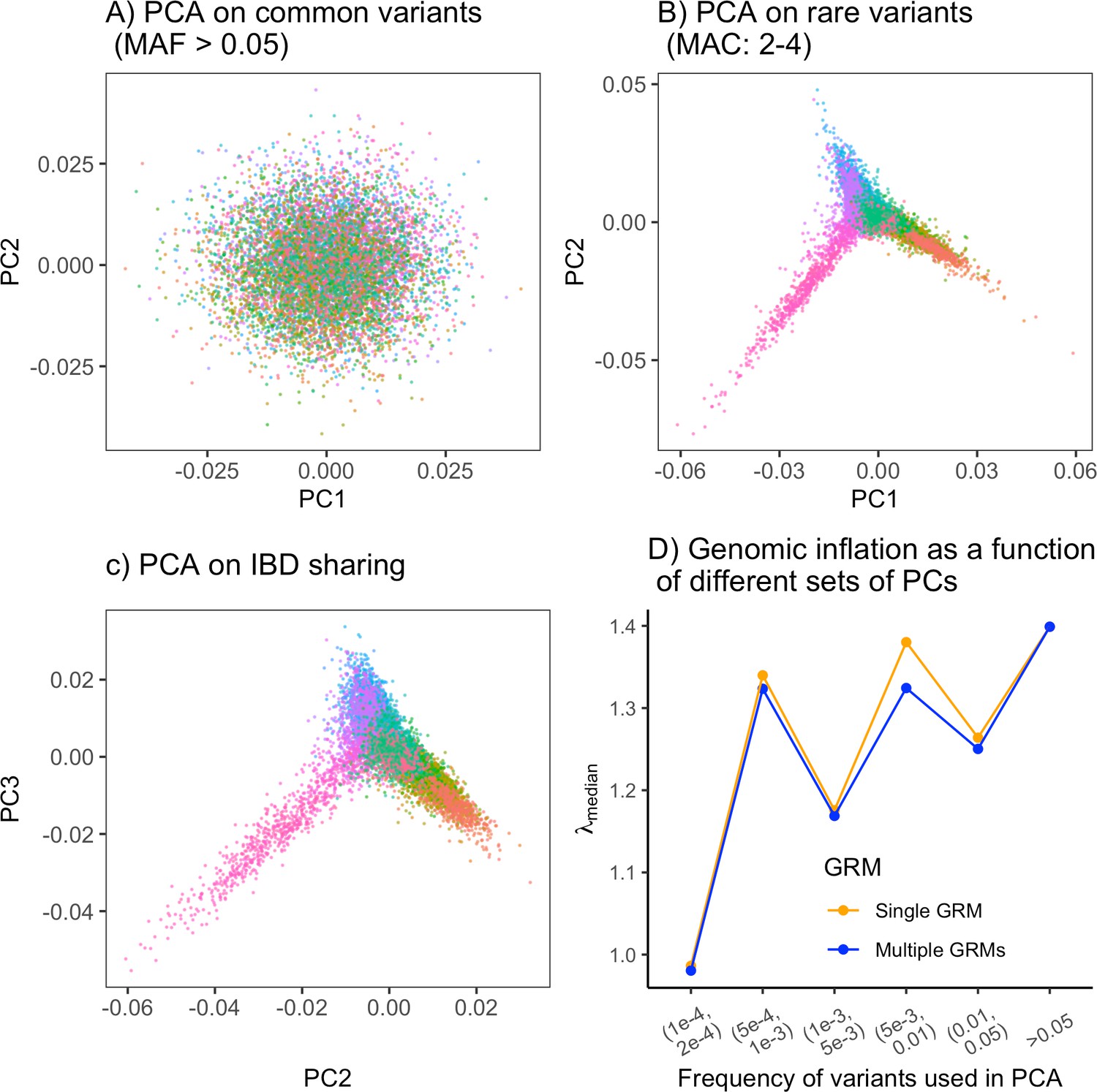
Example of how one might empirically minimize the inflation in test statistic in a genome-wide association study (GWAS) without knowledge of the demographic history.
(A) Principal component analysis (PCA) on common variants shows little or no structure. PCA on (B) rare variants and (C) IBD-sharing captures population structure effectively. (D) Genomic inflation in summary statistics for GWAS on the non-heritable 'Smooth' phenotype as a function of frequency of variants used in PCA. Single genetic relatedness matrix (GRM; orange) refers to the inflation observed with PCs calculated using a single GRM constructed from variants in the given frequency bin. Multiple GRM (blue) refers to the inflation with two sets of PCs calculated separately: 50 PCs from common variants (MAF>0.05) and 50 PCs from variants in the given frequency bin. .
Figure 5—figure supplement 3

PCs computed from a single genetic relatedness matrix (GRM) constructed from common and rare variants together are different in how they capture population stratification than PCs computed from GRMs constructed separately from common and rare variants.
(A) Variance in longitude, latitude, and the sharply distributed phenotype explained by 100 PCs under the complex demographic model. PCs explain more variance in longitude and latitude than in the Sharp phenotype because it is difficult to express the latter as a linear combination of PCs. Note, that PCs explain more variance in latitude than in longitude. This is because under the complex structure model, there is ancestry stratification in the north-south direction in addition to recent structure due to isolation by distance. Importantly, PCs computed separately from common and rare variants explain more of the structure than PCs computed from a single GRM constructed from common and rare variants together. (B) Variance explained in the sharp phenotype.
Figure 6 with 2 supplements
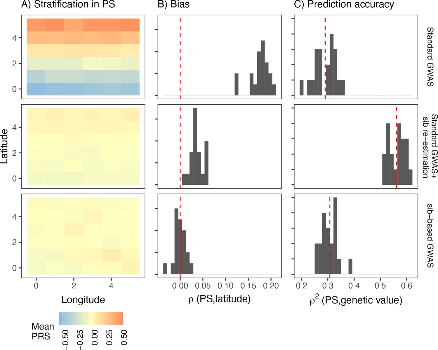
Comparison of stratification and predictive accuracy of polygenic scores between standard and sibling-based association tests under the recent structure model.
Phenotypes simulated as in Figure 4. (A) Spatial distribution of polygenic scores generated using (top) effects of variants discovered in a standard genome-wide association study (GWAS; middle) variants ascertained in a standard GWAS but with effect sizes reestimated in sib-based design, (bottom) variants ascertained and effect sizes estimated in sib-based design. In each case, the effect is averaged over 20 simulations. (B) Bias and (C) predictive accuracy of polygenic scores for 20 simulations of the smooth environmental effect.
Figure 6—figure supplement 1
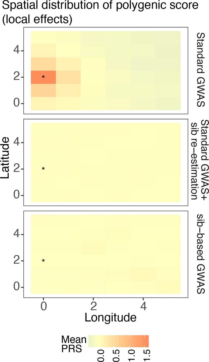
Spatial distribution of residual polygenic scores when the environment is sharply distributed (risk location indicated with *).
The polygenic scores were calculated using variants and their effect sizes in a standard genome-wide association study (GWAS; top row), variants ascertained in a standard GWAS and effects reestimated in sibling pairs (middle row), or a full sibling-based design where both variants and their effects are obtained in sibling pairs. Polygenic scores were averaged across 20 random simulations of the phenotype.
Figure 6—figure supplement 2
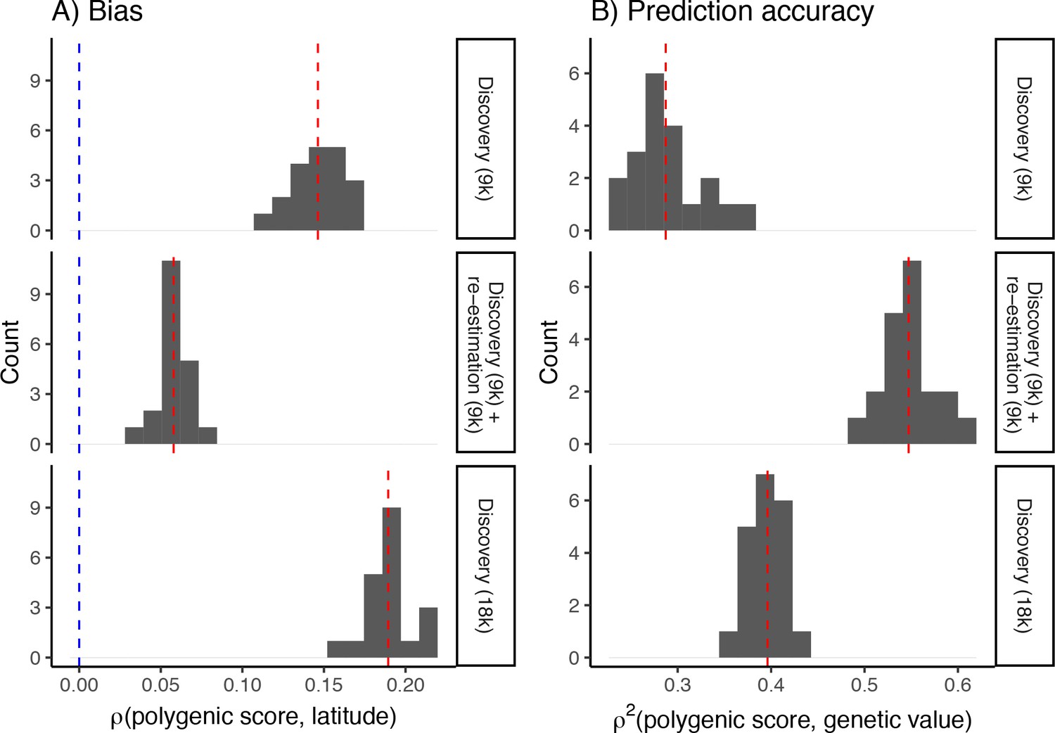
Bias (A) and prediction accuracy (B) of polygenic scores calculated using different variant ascertainment and effect size estimation schemes.
The bias is smallest and prediction accuracy greatest when variants are ascertained in a standard genome-wide association study (GWAS) and their effects reestimated in an independent sample of unrelated individuals (middle row). This explains the bias and prediction accuracy seen when variants were ascertained in a standard GWAS and their effects reestimated in siblings Figure 6. Shown, for comparison, is the bias and prediction accuracy of polygenic scores calculated from effects discovered in a standard GWAS of 9K (top row) and 18K individuals (bottom row), respectively. Even though a larger GWAS improves prediction accuracy slightly, it also increases the bias. Blue dashed lines represent the expected bias and red dashed lines represent the observed mean of the distribution.
Author response image 1
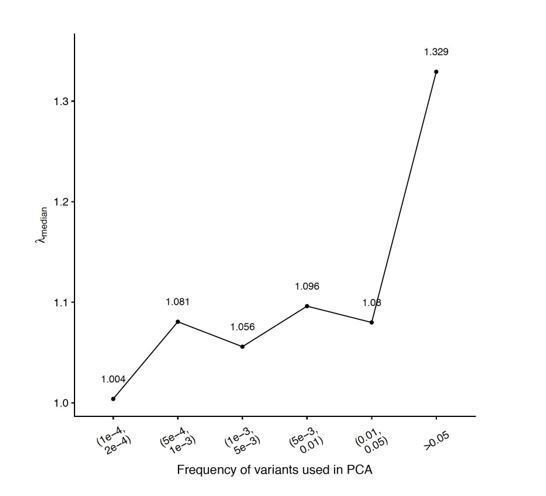
Genomic inflation (y-axis) as a function of variant frequency used to calculate PCs (x-axis).
The GWAS were carried out using genotypes generated under the recent structure model and the smooth phenotype.
Tables
Table 1
Mean observed FST for different migration rate under each demographic model.
| Model | Migration rate1 | Mean FST (95% C.I.) | λ (Latitude) | λ (Longitude) |
|---|---|---|---|---|
| Recent | 0.001 | 3.8e-03 (3.7e-03 - 4e-03) | 3.5649 | 3.7808 |
| Recent | 0.0025 | 2.6e-03 (2.5e-03–2.7e-03) | 3.4733 | 3.6425 |
| Recent | 0.005 | 1.6e-03 (1.5e-03–1.7e-03) | 3.0914 | 3.1357 |
| Recent | 0.0075 | 1.5e-03 (1.4e-03–1.6e-03) | 3.4661 | 3.3344 |
| Recent | 0.01 | 1.1e-03 (1e-03–1.2e-03) | 3.0629 | 3.0675 |
| Recent | 0.015 | 7.9e-04 (7.2e-04–8.6e-04) | 2.8256 | 2.5172 |
| Recent | 0.02 | 7e-04 (6.3e-04–7.7e-04) | 2.4668 | 2.6838 |
| Recent | 0.025 | 5.1e-04 (4.4e-04–5.9e-04) | 2.2173 | 2.6485 |
| Recent | 0.03 | 4e-04 (3.3e-04–4.6e-04) | 2.4842 | 2.2036 |
| Recent | 0.05* | 2.3e-04 (1.7e-04–2.9e-04) | 1.6754 | 1.8486 |
| Perpetual | 0.06 | 2.5e-04 (1.9e-04–3.1e-04) | 1.8101 | 1.7606 |
| Perpetual | 0.07* | 2.0e-04 (1.4e-04–2.6e-04) | 1.6640 | 1.6381 |
| Perpetual | 0.08 | 1.7e-04 (1.1e-04–2.3e-04) | 1.5905 | 1.6658 |
| Complex | 0.05 | 3.2e-04 (2.5e-04–3.8e-04) | 2.6425 | 1.7480 |
| Complex | 0.06 | 2.8e-04 (2.1e-04–3.4e-04) | 2.1651 | 1.8637 |
| Complex | 0.07 | 2.5e-04 (1.8e-04–3.1e-04) | 1.9318 | 1.7012 |
| Complex | 0.08* | 1.5e-04 (9.7e-05–2.1e-04) | 1.6520 | 1.5214 |
| Complex | 0.09 | 1.7e-04 (1.1e-04–2.2e-04) | 1.6841 | 1.3892 |
| Complex | 0.1 | 1.7e-04 (1.2e-04–2.3e-04) | 1.5943 | 1.4719 |
| Complex | 0.12 | 1.3e-04 (7.3e-05–1.8e-04) | 1.4442 | 1.4395 |
| Complex | 0.15 | 7.9e-05 (2.7e-05–1.3e-04) | 1.2536 | 1.3123 |
-
Proportion of migrants in and out of a deme per generation. Selected migration rate indicated with * for each model.
Additional files
Download links
A two-part list of links to download the article, or parts of the article, in various formats.
Downloads (link to download the article as PDF)
Open citations (links to open the citations from this article in various online reference manager services)
Cite this article (links to download the citations from this article in formats compatible with various reference manager tools)
Demographic history mediates the effect of stratification on polygenic scores
eLife 9:e61548.
https://doi.org/10.7554/eLife.61548


