Genetic disruption of WASHC4 drives endo-lysosomal dysfunction and cognitive-movement impairments in mice and humans
- Department of Neurobiology, Duke University School of Medicine, United States
- Proteomics and Metabolomics Shared Resource, Duke University School of Medicine, United States
- Department of Cell Biology, Duke University School of Medicine, United States
- Burjeel Hospital, VPS Healthcare, Oman
- Department of Pathology, Duke University School of Medicine, United States
- Department of Anatomy and Neurobiology, University of Tennessee Heath Science Center, United States
Figures
Figure 1 with 1 supplement
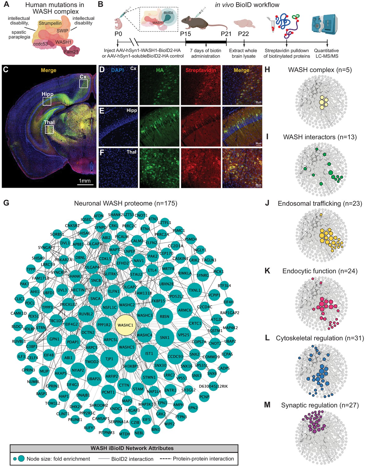
Identification of the WASH complex proteome in vivo.
(A) The WASH complex is composed of five subunits: Washc1 (WASH1), Washc2 (FAM21), Washc3 (CCDC53), Washc4 (SWIP), and Washc5 (Strumpellin). Human mutations in these components are associated with spastic paraplegia (de Bot et al., 2013; Jahic et al., 2015; Valdmanis et al., 2007), Ritscher–Schinzel syndrome (Elliott et al., 2013), and intellectual disability (Assoum et al., 2020; Ropers et al., 2011). (B) A BioID2 probe was attached to the c-terminus of WASH1 and expressed under the human synapsin-1 (hSyn1) promoter in an AAV construct for in vivo BioID (iBioID). iBioID probes (WASH1-BioID2-HA or negative control solubleBioID2-HA) were injected into wild-type mouse brain at P0 and allowed to express for 2 weeks. Subcutaneous biotin injections (24 mg/kg) were administered over 7 days for biotinylation, and then brains were harvested for isolation and purification of biotinylated proteins. LC–MS/MS identified proteins significantly enriched in all three replicates of WASH1-BioID2 samples over soluble-BioID2 controls. (C) Representative image of WASH1-BioID2-HA expression in a mouse coronal brain section (Cx=cortex, Hipp=hippocampus, Thal=thalamus). Scale bar, 1 mm. (D) Representative image of WASH1-BioID2-HA expression in mouse cortex (inset from C). Individual panels show nuclei (DAPI, blue), AAV construct HA epitope (green), and biotinylated proteins (Streptavidin, red). Merged image shows colocalization of HA and Streptavidin (yellow). Scale bar, 50 µm. (E) Representative image of WASH1-BioID2-HA expression in mouse hippocampus (inset from C). Scale bar, 50 µm. (F) Representative image of WASH1-BioID2-HA expression in mouse thalamus (inset from C). Scale bar, 50 µm. (G) iBioID identified 175 proteins in the WASH interactome (fold-enrichment>4; FDR<0.05). Node size represents protein abundance fold-enrichment over negative control (range: 4–7.5), solid gray edges delineate iBioID interactions between the WASHC1 probe (seen in yellow at the center) and identified proteins, and dashed edges indicate known protein–protein interactions from HitPredict database (López et al., 2015). (H,I) Clustergrams of (H) all five WASH complex proteins identified by iBioID. (I) Previously reported WASH interactors (13/175), including the CCC and Retriever complexes. (J) Endosomal trafficking proteins (23/175 proteins). (K) Endocytic proteins (24/175). (L) Proteins involved in cytoskeletal regulation (31/175), including Arp2/3 subunit, ARPC5. (M) Synaptic proteins (27/175). Clustergrams were annotated by hand and cross-referenced with Metascape GO enrichment (Zhou et al., 2019) of WASH1 proteome constituents over all proteins identified in the BioID experiment.
Figure 1—figure supplement 1
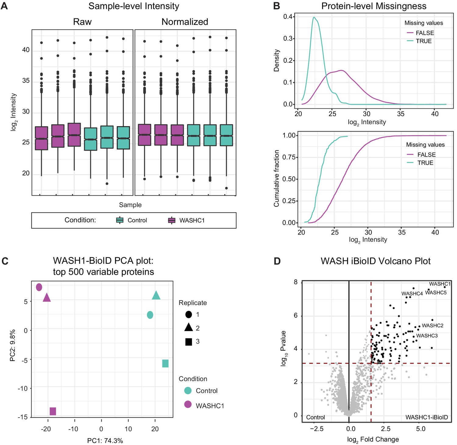
In vivo BioID data normalization and analysis parameters.
(A) After normalization, protein intensity is not different between SolubleBioID2 Control and WASHC1-BioID2 samples. Control samples are depicted in teal, WASH1 samples are depicted in purple. Data reported as mean ± SD, error bars are SD, n=3 independent experiments. (B) Protein-level missingness is inferred to be missing not-at-random due to the left shifted distribution of the density distributions of proteins with missing values. Top: Density distribution. Bottom: Cumulative distribution. (C) Principal component analysis (PCA) of Control and WASHC1 samples reveals clear separation of experimental conditions. (D) Volcano plot of proteins identified in in vivo BioID experiment illustrates the thresholds used to consider proteins significantly enriched in WASHC1 samples over Control: Fold-change≥4.0, Benjamini–Hochberg FDR<0.05, p<0.05. All five WASH complex proteins were significantly enriched.
Figure 2 with 1 supplement
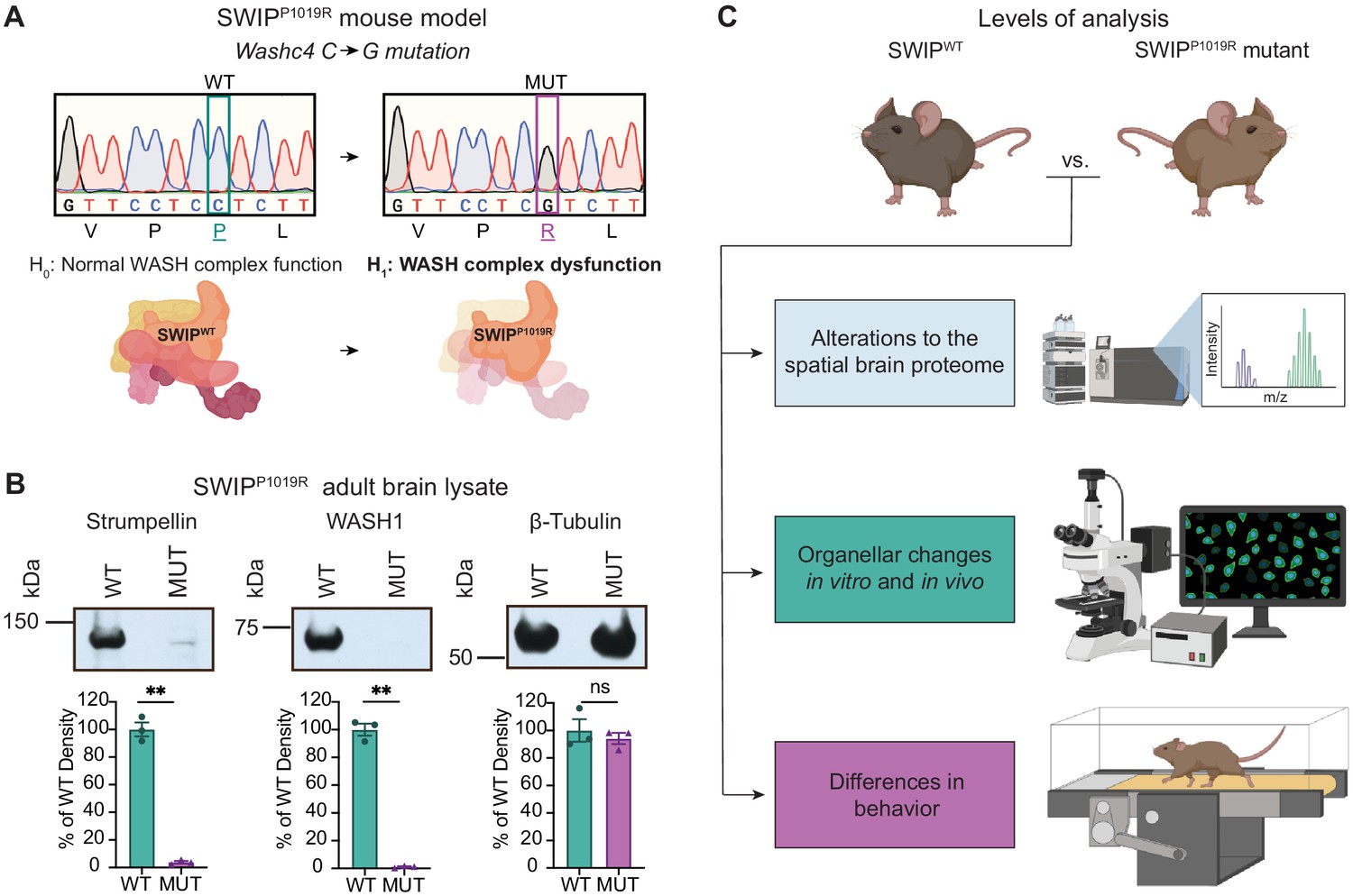
Mouse model of the human SWIPP1019R mutation displays decreases in WASH complex components.
(A) Mouse model of the human SWIPP1019R missense mutation created using CRISPR. A C>G point mutation was introduced into exon29 of murine Washc4, leading to a P1019R amino acid substitution. We hypothesize (H1) that this mutation causes instability of the WASH complex. (B) Representative western blot and quantification of WASH components, Strumpellin and WASH1 (predicted sizes in kDa: 134 and 72, respectively), as well as loading control β-tubulin (55 kDa) from adult whole-brain lysate prepared from SWIP WT (Washc4C/C) and SWIP homozygous MUT (Washc4G/G) mice. Bar plots show quantification of band intensities normalized to β-tubulin, expressed as a % of WT (n=3 mice per genotype). Strumpellin (WT 100.0±5.1%, MUT 3.8±0.9%, t2.14=18.60, p=0.0021) and WASH1 (WT 100.0±4.3%, MUT 1.1±0.4%, t2.1=22.77, p=0.0018) were significantly decreased. Equivalent amounts of protein were analyzed in each condition (β-tubulin: WT 100.0±8.2%, MUT 94.1±4.1%, U=4, p>0.99). (C) Schematic of experimental techniques used to interrogate the effect of the SWIPP1019R mutation in subsequent figures: spatial proteomics (top), confocal and electron microscopy (middle), and mouse behavioral tasks (bottom).
Figure 2—figure supplement 1
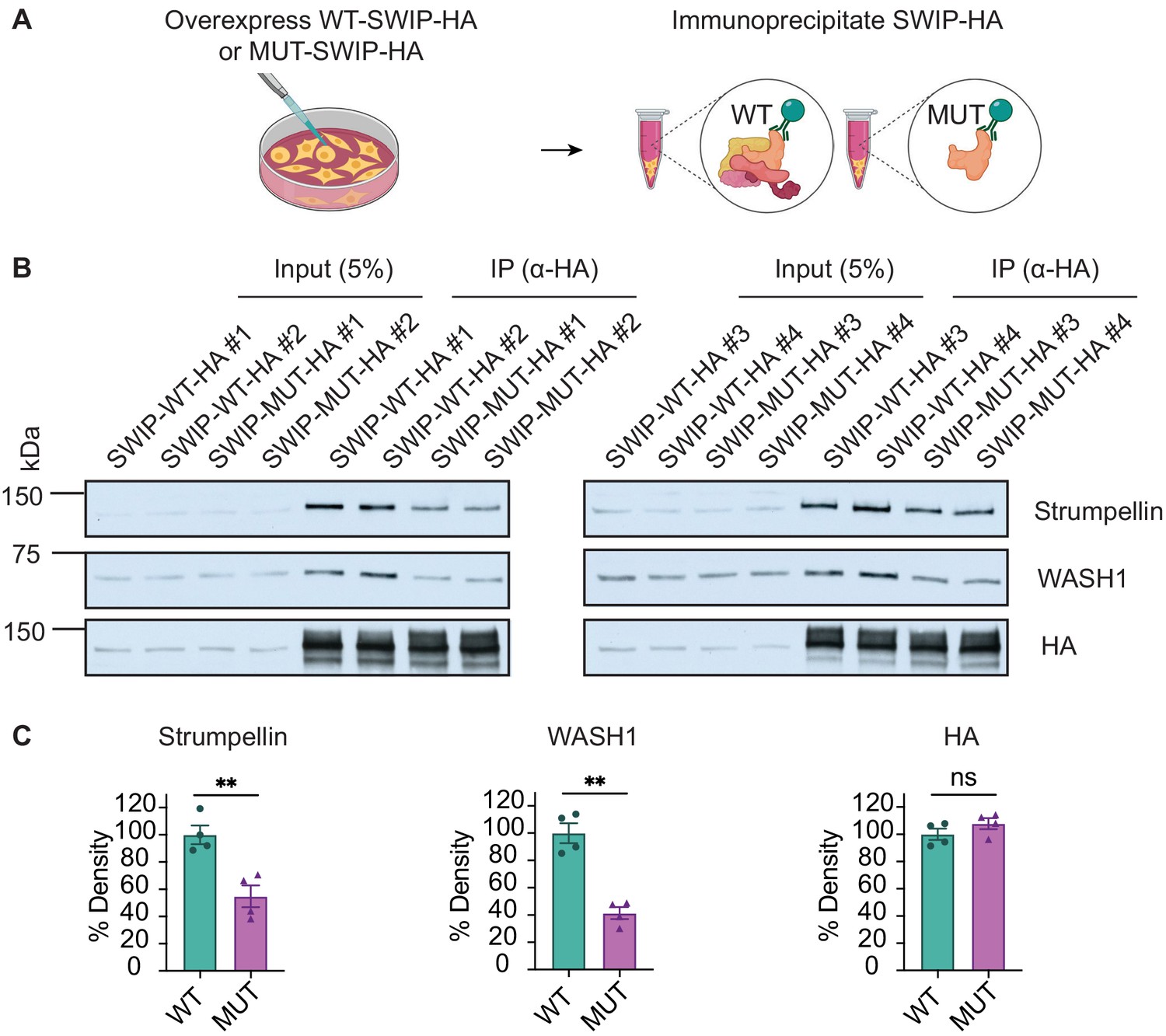
Overexpression of SWIPP1019R decreases WASH complex binding in cultured cells.
(A) Schematic showing overexpression of WT or MUT SWIPP1019R in HEK293T cells followed by immunoprecipitation. (B) Western blots of input (5%, left) and immunoprecipitated (IP, right) protein. Two samples per condition were run on two separate gels, n=4 separate experiments. (C) Quantification of B normalized to WT. Strumpellin (WT 100.0±6.8%, MUT 54.8±8.0%, t5.9=4.290, p=0.0054), WASH1 (WT 100.0±7.3%, MUT 41.4±4.4%, t4.9=6.902, p=0.0011), HA (WT 100.0±4.1%, MUT 107.8±4.1%, t6.0=1.344, p=0.2275). Data reported as mean ± SEM, error bars are SEM. **p<0.01, two-tailed t-tests.
Figure 3 with 5 supplements

Spatial proteomics and network covariation analysis reveal significant disruptions to the WASH complex and an endosomal module in SWIPP1019R mutant mouse brain.
(A) Tandem-mass-tag (TMT) spatial proteomics experimental design. Seven subcellular fractions were prepared from one WT and one MUT mouse (10mo). These samples, as well as two pooled quality control (QC) samples, were labeled with unique TMT tags and concatenated for simultaneous 16-plex LC–MS/MS analysis. This experiment was repeated three times (three WT and three MUT brains total). To detect network-level changes, proteins were clustered into modules, and linear mixed models (LMMs) were used to identify differences in module abundance between WT and MUT conditions. The network shows an overview of the spatial proteomics graph in which 49 different modules are indicated by colored nodes. (B) Protein module 38 (M38) contains subunits of the WASH, CCC, Retriever, and CORVET/HOPS complexes. Node size denotes its weighted degree centrality (~importance in module); purple node color indicates proteins with altered abundance in MUT brain relative to WT; red, yellow, orange, and green node borders highlight protein components of the CCC, Retriever, CORVET/HOPS, and WASH complexes obtained from the CORUM database; dashed black edges indicate experimentally determined protein-protein interactions; and gray-red edges denote the relative strength of protein covariation within a module (gray=weak, dark red=strong). (C) M38 displays decreased overall abundance in MUT brain. The aligned profiles of all M38 proteins are plotted together after sum normalization, and rescaling such that the maximum intensity is 1. Each solid line represents a single protein, measured in WT (teal) and MUT (purple) conditions. The estimated WT and MUT means are displayed in dashed teal and purple lines, respectively (WT-MUT Contrast log2Fold-Change=−0.12, T=−11.14, DF=2324, p-adjust=2.078×10⁻²⁶; n=3 independent experiments). (D) Protein profile of WASHC4 (aka SWIP) plotted as relative (sum-normalized) protein intensity, rescaled to be in the range of 0–1 (WT-MUT Contrast log2Fold-Change=−1.517, DF=26, p-adjust=1.72×10⁻¹⁶; n=3 independent experiments). WT levels are depicted in teal, and MUT levels are depicted in purple. Shaded error bar represents the min-to-max values of all three experimental replicates. Significant differences in individual BioFraction WASHC4 levels are indicated with stars. ***p<0.001, MSstatsTMT p-value for intra-BioFraction comparisons with FDR correction.
Figure 3—figure supplement 1

Western blot analysis of LAMP1 abundance across subcellular brain fractions.
(A) Line graph depicting LAMP1 signal abundance normalized to total protein across subcellular biological fractions. LAMP1 pattern reveals no difference between MUT and WT in LAMP1 pelleting, but a significant difference in the abundance of LAMP1 in BioFraction 8 (two-way ANOVA genotype effect, F4,44=7.68, p<0.0001; Sidak’s multiple comparisons test, p=0.0006). Shaded region highlights subcellular fractions used in 16-plex TMT mass spectrometry experiments. Fractions 4–10 from one WT and one MUT mouse were analyzed for each TMT experiment. Data reported as mean ± SEM, error bars are SEM. (B) Western blots depicting LAMP1 abundance from three separate WT animals (Experiments 1–3). (C) Western blots depicting LAMP1 abundance from three separate MUT animals (Experiments 1–3).
Figure 3—figure supplement 2

Western blot analysis of EEA1 abundance across subcellular brain fractions.
(A) Line graph depicting EEA1 signal abundance normalized to total protein across subcellular biological fractions. EEA1 pattern reveals no difference between MUT and WT in EEA1 pelleting (two-way ANOVA genotype effect, F1,4=0.290, p=0.6184). Shaded region highlights subcellular fractions used in 16-plex TMT mass spectrometry experiments. Fractions 4–10 from one WT and one MUT mouse were analyzed for each TMT experiment. Data reported as mean ± SEM, error bars are SEM. (B) Western blots depicting EEA1 abundance from three separate WT animals (Experiments 1–3). (C) Western blots depicting EEA1 abundance from three separate MUT animals (Experiments 1–3).
Figure 3—figure supplement 3
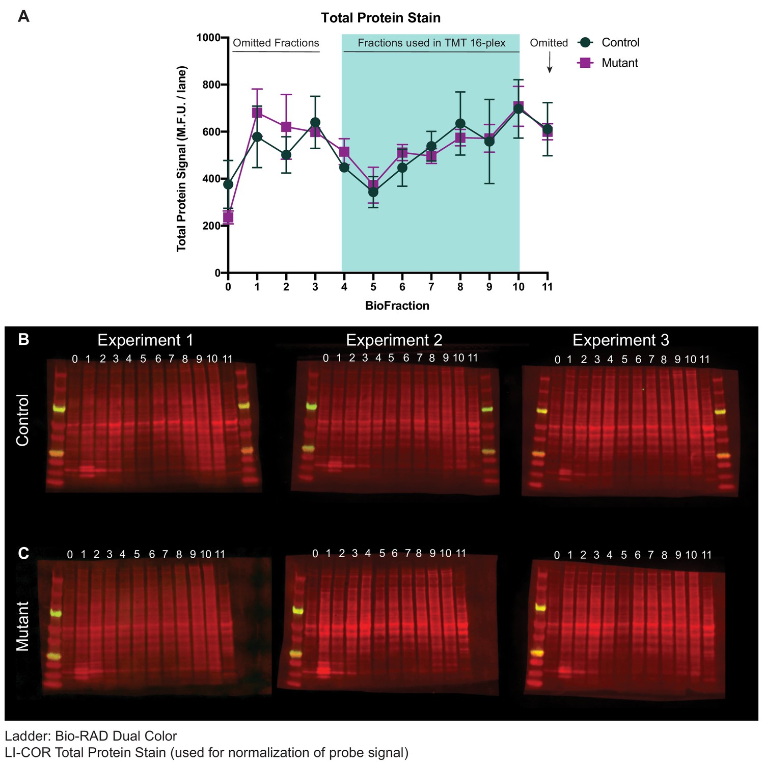
Western blot analysis of total protein abundance across subcellular brain fractions.
(A) Line graph depicting total protein abundance across subcellular biological fractions. There is no difference between MUT and WT samples (two-way ANOVA genotype effect, F1,4=0.0094, p=0.9274), measured by mean fluorescence units (M.F.U.) per lane. Shaded region highlights subcellular fractions used in 16-plex TMT mass spectrometry experiments. Fractions 4–10 from one WT and one MUT mouse were analyzed for each TMT experiment. Data reported as mean ± SEM, error bars are SEM. (B) Western blots of total protein abundance across subcellular fractions from three separate WT animals (Experiments 1–3). (C) Western blots of total protein abundance across subcellular fractions from three separate MUT animals (Experiments 1–3). Total protein abundance per lane was used for normalizing endosomal and lysosomal markers.
Figure 3—figure supplement 4
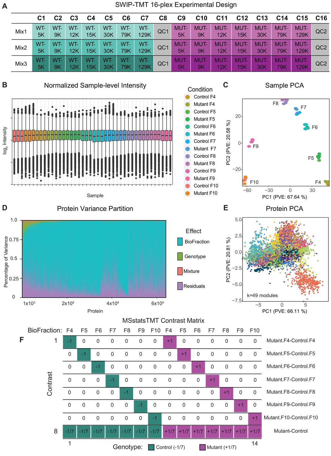
Spatial proteomics experimental design and data analysis.
(A) Experimental design used for tandem-mass-tag (TMT) spatial proteomics. Each experiment was designated as a mixture (Mix 1–3), with seven BioFractions prepared from one WT and one MUT animal (TMT channels: C1–7=WT; C9–15=MUT). The g-force pelleting speed used to obtain each BioFraction is indicated in the corresponding square (i.e. 5K=5000xg). Two sample-pooled quality control samples were used for normalization between experiments in channels 8 and 16 (QC1 and QC2). (B) Boxplot of protein intensity for all proteins in each sample showing no large differences within or between batches after normalization. (C) Principal component analysis of each sample reveals separation of all 7 BioFractions. (D) The variance attributable to the experiments’ major covariates for every protein. After normalization, the major source of variation for most proteins is BioFraction. After normalization, the variation attributable to differences between mixtures is negligible. (E) Principal component analysis of proteins showing the 49 modules identified by clustering the spatial proteomics network. (F) Matrix of comparisons used by MSstatsTMT to assess intra-BioFraction and overall protein differences between Control and Mutant conditions.
Figure 3—figure supplement 5

Analysis of spatial brain proteome reveals conservation of organellar compartments found in LOPIT-DC dataset.
(A) Module 4 is 5.6-fold enriched for plasma membrane proteins (p-adjust=1.39×10−38) and displays no significant change in module-level intensity between WT and MUT conditions (p-adjust=0.323). (B) Module 5 is 2.4-fold enriched for nuclear proteins (p-adjust=3.48×10⁻²²) and displays no significant change in module-level intensity between WT and MUT conditions (p-adjust=0.270). (C) Module 1 is 6.7-fold enriched for cytosolic proteins (p-adjust=1.06×10−89) and displays a slight change in module-level intensity between WT and MUT conditions (p-adjust=6.5×10⁻²⁰). (D) Module 13 is 6.1-fold enriched for ribosomal proteins (p-adjust=2.0×10⁻¹⁰) and displays no significant change in module-level intensity between WT and MUT conditions (p-adjust=1). (E) Module 7 is 4.7-fold enriched for endoplasmic reticulum proteins (p-adjust=8.43×10⁻¹⁶) and displays no significant change in module-level intensity between WT and MUT conditions (p-adjust=1). (F) Module 40 is 6.8-fold enriched for mitochondrial proteins (p-adjust=5.40×10⁻¹⁵) and displays a slight change in module-level intensity between WT and MUT conditions (p-adjust=8.18×10⁻⁶). (G) Module 9 is 18.5-fold enriched for peroxisomal proteins (p-adjust=1.39×10⁻²⁰) and displays no significant change in module-level intensity between WT and MUT conditions (p-adjust=0.474). (H) Module 8 is 27.6-fold enriched for proteasomal proteins (p-adjust=7.91×10−41) and displays no significant change in module-level intensity between WT and MUT conditions (p-adjust=1). For all modules, light purple nodes represent proteins with decreased abundance in MUT samples, dark purple nodes represent proteins with increased abundance in MUT samples, blue node borders highlight proteins with sample organelle designation as (Geladaki et al., 2019), experimentally determined protein–protein interactions (HitPredict), and gray-red edges denote the relative strength of protein covariation within a module (gray=weak, dark red=strong). Corresponding profile plots for each module depict individual scaled protein intensities in light teal (WT) and purple (MUT) lines, with the estimated value of WT and MUT conditions shown as dashed lines.
Figure 4 with 2 supplements
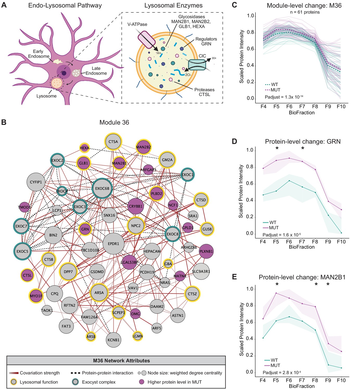
Disruption of a lysosomal protein network in SWIPP1019R mutant brain.
(A) Simplified schematic of the endo-lysosomal pathway in neurons. Inset depicts representative lysosomal enzymes, such as proteases (CTSL), glycosidases (MAN2B1, MAN2B2, GLB1, HEXA), and key lysosomal regulators (GRN). (B) Network graph of module 36 (M36). M36 proteins that exhibit altered abundance in MUT brain include lysosomal proteins, HEXA, GLB1, MAN2B1, MAN2B2, GRN, and CTSL. Network attributes: Node size denotes its weighted degree centrality (~importance in module), node color indicates proteins with altered abundance in MUT brain relative to WT, yellow outlines highlight proteins identified as lysosomal in Geladaki et al., 2019, green outlines indicate members of the exocyst complex (CORUM), dashed black edges indicate experimentally determined protein-protein interactions (HitPredict), and gray-red edges denote the relative strength of protein covariation within a module (gray=weak, dark red=strong). (C) The scaled protein intensity of all M36 proteins plotted together as a module. Overall, there is a significant increase in the estimated mean of M36 relative to WT (WT-MUT log2Fold-Change=0.086, T=8.25, DF=2488, p-adjust=1.29×10⁻¹⁴; n=3 independent experiments). Light teal and purple lines denote scaled protein profiles for individual WT and MUT proteins, respectively. Dashed green and purple lines indicate mean scaled protein intensities for WT and MUT, respectively. (D) Protein profile of lysosomal protein progranulin, GRN (WT-MUT Contrast log2Fold-Change=0.637, DF=28, p-adjust=1.58×10⁻⁵; n=3 independent experiments). (E) Protein profile of lysosomal enzyme, MAN2B1 (WT-MUT Contrast log2Fold-Change=0.319, DF=26, p-adjust=2.75×10⁻⁴; n=3 independent experiments). For (D) and (E), WT levels are depicted in teal, and MUT levels are depicted in purple. Shaded error bar represents the min-to-max values of all three experimental replicates. Significant differences in individual BioFraction levels are indicated with stars. *p<0.05, MSstatsTMT p-value for intra-BioFraction comparisons with FDR correction (D,E).
Figure 4—figure supplement 1
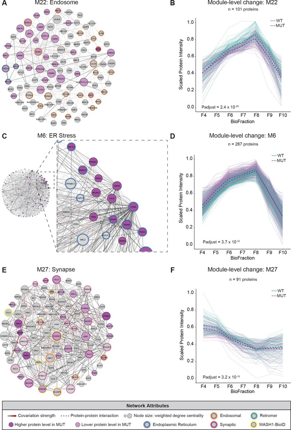
Multiple protein networks display significant alterations in MUT brain compared to WT.
(A) Network graph of Module 22 (M22) containing endosomal proteins from UniProt. Three retromer sorting complex subunits (CORUM) are highlighted with teal borders and endosomal proteins are highlighted with orange borders. For all networks, light purple nodes denote proteins whose abundance is decreased in MUT samples, dark purple nodes denote proteins whose abundance is increased in MUT samples, node size reflects weighted degree centrality (~importance in network), dashed black lines denote protein–protein interactions, and gray-red lines indicate covariation strength (gray=weak, dark red=strong). (B) Module-level profile of scaled M22 protein intensity reveals decreased abundance in MUT samples compared to WT (WT-MUT log2Fold-Change=−0.095, T=−11.5, DF=4128, p-adjust=2.42×10⁻²⁸; n=3 independent experiments). For all profile plots, light teal lines denote individual WT protein levels, light purple lines denote individual MUT protein levels, dashed green lines represent estimated WT scaled intensity, and dashed purple lines represent estimated MUT scaled intensity. (C) Network graph of Module 6 (M6) containing endoplasmic reticulum proteins. Inset highlights multiple proteins involved in the ER stress response. Proteins which were also designated as ER localized in the dataset by Geladaki et al., 2019 are highlighted with blue borders. (D) Profile of M6. Overall, there is a significant increase in MUT conditions compared to WT (WT-MUT log2Fold-Change=0.059, T=12.2, DF=10934, p-adjust=3.68×10⁻³²; n=3 independent experiments). (E) Network graph of Module 27 (M27) containing synaptic proteins. Synaptic proteins are highlighted with pink node borders, and proteins that were also identified as enriched in the WASH1-BioID2 proteome (Figure 1) are highlighted with yellow node borders. (F) Module-level profile plotting scaled protein intensities of M27 constituents. Overall, there is a significant decrease in MUT conditions compared to WT (WT-MUT log2Fold-Change=−0.059, T=−6.89, DF=3718, p-adjust=3.19×10⁻¹⁰; n=3 independent experiments).
Figure 4—figure supplement 2

Aged SWIPP1019R mutant mice display decreased excitatory synapse number in the motor cortex.
(A) Schematic representation of brain region analyzed, motor cortex, adapted from Allen Brain Atlas (Oh et al., 2014). (B,C) Representative images of excitatory synaptic staining in adolescent WT (B) and MUT (C) brain. Excitatory pre-synaptic marker, bassoon, is depicted in magenta and excitatory post-synaptic marker, homer1, is depicted in green. Their colocalization is visualized as white puncta. (D) Graph of the average number of synaptic puncta per 250×250 µm region of interest, normalized to percent of WT (WT 100.0±3.5, n=18 regions of interest (ROIs;) MUT 97.36±3.3, n=18 ROIs; t33.9=0.5509, p=0.5853). (E,F) Representative images of excitatory synaptic staining in aged adult WT (E) and MUT (F) brain. (G) Graph of the average number of synaptic puncta per 250×250 µm region of interest, normalized to percent of WT (WT 100.0±3.4, n=18 ROIs; MUT 80.80±2.4, n=18 ROIs; t30.9=4.599, p<0.0001). Analyses included three separate animals per condition. Scale bars, 5 µm (B–F). Data reported as mean ± SEM, error bars are SEM. ****p<0.0001, two-tailed t-tests.
Figure 5
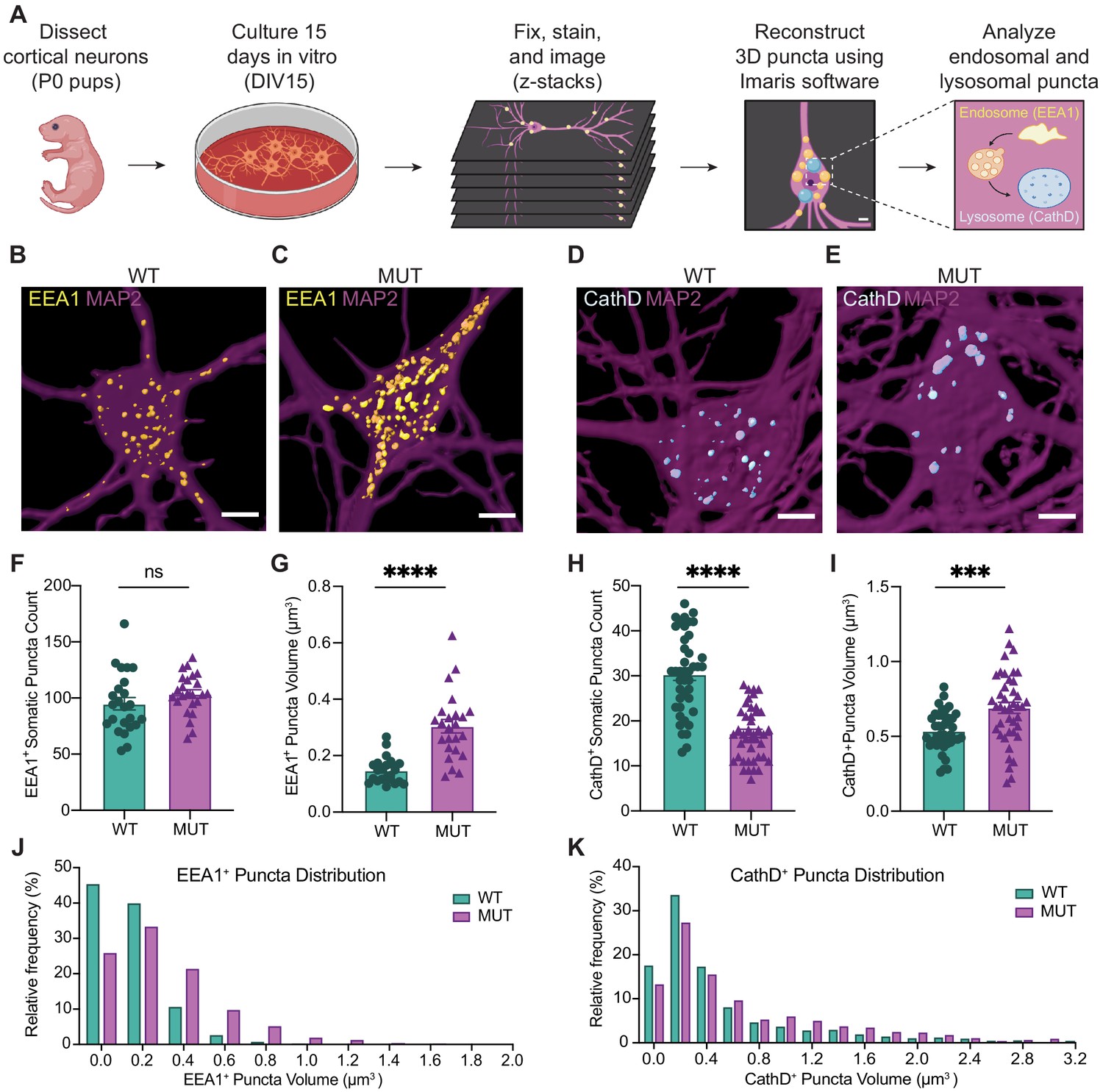
SWIPP1019R mutant neurons display structural abnormalities in endo-lysosomal compartments in vitro.
(A) Experimental design. Cortices were dissected from P0 pups, and neurons were dissociated and cultured on glass coverslips for 15 days. Cultures were fixed, stained, and imaged using confocal microscopy. 3D puncta volumes were reconstructed from z-stack images using Imaris software. (B,C) Representative 3D reconstructions of WT and MUT DIV15 neurons (respectively) stained for EEA1 (yellow) and MAP2 (magenta). (D,E) Representative 3D reconstructions of WT and MUT DIV15 neurons (respectively) stained for Cathepsin D (cyan) and MAP2 (magenta). (F) Graph of the average number of EEA1+ volumes per soma in each image (WT 95.0±5.5, n = 24 neurons; MUT 103.7±3.7, n = 24 neurons; U = 208.5, p=0.1024). (G) Graph of the average EEA1+ volume size per soma shows larger EEA1+ volumes in MUT neurons (WT 0.15±0.01 µm3, n=24 neurons; MUT 0.30±0.02 µm3, n=24 neurons; U=50, p<0.0001). (H) Graph of the average number of Cathepsin D+ volumes per soma illustrates less Cathepsin D+ volumes in MUT neurons (WT 30.4±1.4, n=42; MUT 17.2±0.9, n=42; U=204, p<0.0001). (I) Graph of the average Cathepsin D+ volume size per soma demonstrates larger Cathepsin D+ volumes in MUT neurons (WT 0.54±0.02 µm3, n=42; MUT 0.69±0.04 µm3, n=42; t63=3.701, p=0.0005). (J) Histogram of EEA1+ volumes illustrate differences in size distributions between MUT and WT neurons (D=0.2661, p<0.0001). (K) Histogram of CathD+ volumes show differences in size distributions between MUT and WT neurons (D=0.1307, p<0.0001). Analyses included at least three separate culture preparations. Scale bars, 5 µm (B–E). Data reported as mean ± SEM, error bars are SEM. ***p<0.001, ****p<0.0001, Mann–Whitney U test (F–H), two-tailed t-test (I), or Kolmogorov–Smirnov test (J,K).
Figure 6 with 2 supplements
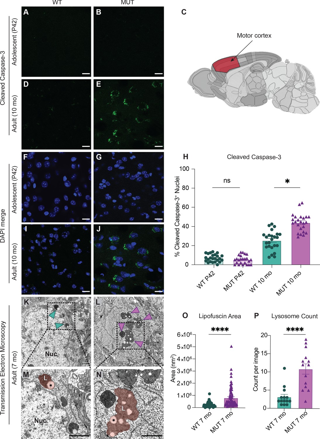
SWIPP1019R mutant brains exhibit markers of abnormal endo-lysosomal structures and cell death in vivo.
(A,B) Representative images of adolescent (P42) WT and MUT motor cortex stained with cleaved caspase-3 (CC3, green). (C) Anatomical representation of mouse brain with motor cortex highlighted in red, adapted from the Allen Brain Atlas (Oh et al., 2014). (D,E) Representative image of adult (10 mo) WT and MUT motor cortex stained with CC3 (green). (F, G, I, and J) DAPI co-stained images for (A, B, D, and E, respectively). Scale bar for (A–J), 15 µm. (H) Graph depicting the normalized percentage of DAPI+ nuclei that are positive for CC3 per image. No difference is seen at P42, but the amount of CC3+ nuclei is significantly higher in aged MUT mice (P42 WT 6.97 ± 0.80%, P42 MUT 5.26 ± 0.90%, 10mo WT 25.38 ± 2.05%, 10mo MUT 44.01 ± 1.90%, H=74.12, p<0.0001). We observed no difference in number of nuclei per image between genotypes. (K) Representative transmission electron microscopy (TEM) image taken of soma from adult (7mo) WT motor cortex. Arrowheads delineate electron-dense lipofuscin material, Nuc=nucleus. (L) Representative transmission electron microscopy (TEM) image taken of soma from adult (7mo) MUT motor cortex. (M) Inset from (K) highlights lysosomal structure in WT soma. Pseudo-colored region depicts lipofuscin area, demarcated as L. (N) Inset from (L) highlights large lipofuscin deposit in MUT soma (L, pseudo-colored region) with electron-dense and electron-lucent lipid-like (asterisk) components. (O) Graph of areas of electron-dense regions of interest (ROI) shows increased ROI size in MUT neurons (WT 2.4×10⁵ ± 2.8×10⁴ nm2, n=50 ROIs; MUT 8.2×10⁵±9.7×10⁴ nm2, n=75 ROIs; U=636, p<0.0001). (P) Graph of the average number of presumptive lysosomes with associated electron-dense material reveals increased number in MUT samples (WT 3.14±0.72 ROIs, n=14 images; MUT 10.86 ± 1.42 ROIs, n=14 images; U=17, p<0.0001). For (O) and (P), images were taken from multiple TEM grids, prepared from n=3 animals per genotype. Scale bar for all TEM images, 1 µm. Data reported as mean ± SEM, error bars are SEM. *p<0.05, ****p<0.0001, Kruskal–Wallis test (H), Mann–Whitney U test (O,P).
Figure 6—figure supplement 1
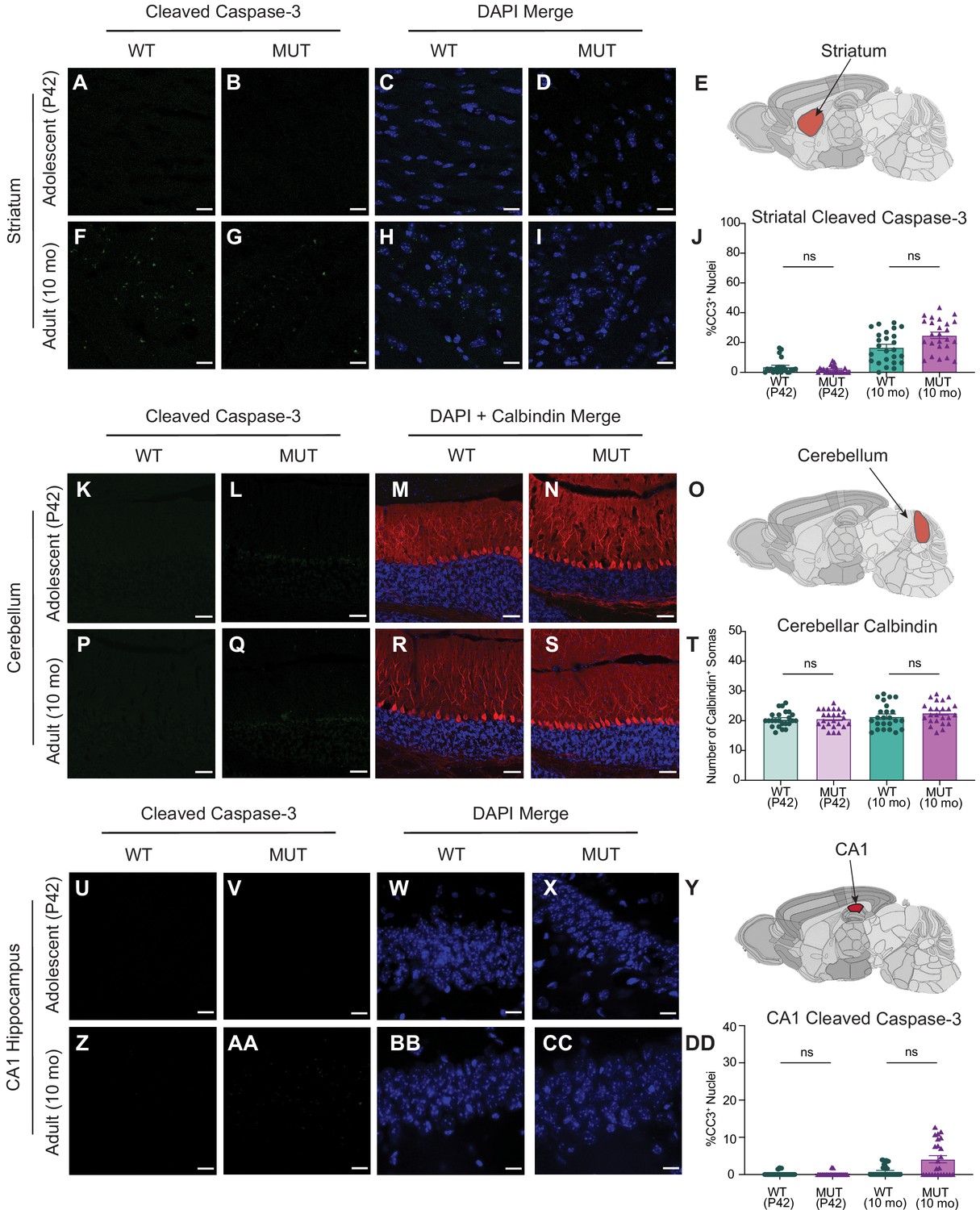
There is no significant difference in striatal, cerebellar, or hippocampal cell death between WT and MUT mice.
(A) Representative image of adolescent (P42) WT striatum stained with cleaved caspase-3 (CC3, green). (B) Representative image of adolescent (P42) MUT striatum stained with cleaved caspase-3 (CC3, green). (C,D) DAPI co-stained images of A and B, respectively. (E) Anatomical representation of mouse brain with striatum highlighted in red, adapted from the Allen Brain Atlas (Oh et al., 2014). (F) Representative image of adult (10 mo) WT striatum stained with CC3 (green). (G) Representative image of adult (10 mo) MUT striatum stained with CC3 (green). (H,I) DAPI co-stained images of F and G, respectively. Scale bars for A-I are 15 µm. (J) Graph depicting the normalized % of DAPI+ nuclei that are positive for CC3 per image. No difference is seen between genotypes at either age (P42 WT 3.70 ± 0.99%, P42 MUT 1.95 ± 0.49%, 10mo WT 16.77 ± 2.09%, 10mo MUT 24.86 ± 2.17%, H=61.87, p<0.0001). (K) Representative image of adolescent (P42) WT cerebellum stained with cleaved caspase-3 (CC3, green). (L) Representative image of adolescent (P42) MUT cerebellum stained with cleaved caspase-3 (CC3, green). (M,N) DAPI and Calbindin co-stained images of K and L, respectively. (O) Anatomical representation of mouse cerebellum, adapted from the Allen Brain Atlas (Oh et al., 2014). Red region highlights area used for imaging. (P) Representative image of adult (10 mo) WT cerebellum stained with CC3 (green). (Q) Representative image of adult (10 mo) MUT cerebellum stained with CC3 (green). No significant CC3 staining is observed at either age. (R,S) DAPI and Calbindin co-stained images of P and Q, respectively. Scale bars for K-S are 50 µm. (T) Graph depicting the number of Calbindin+ somas per image, a marker for Purkinje cells. No difference is seen between genotypes at either age (P42 WT 20.50 ± 0.53, P42 MUT 20.67 ± 0.59, 10mo WT 21.42 ± 0.85, 10mo MUT 22.63 ± 0.74, H=4.891, p=0.1799). (U) Representative image of adolescent (P42) WT hippocampus stained with cleaved caspase-3 (CC3, green). (V) Representative image of adolescent (P42) MUT hippocampus stained with cleaved caspase-3 (CC3, green). (W,X) DAPI co-stained images of U and V, respectively. (Y) Anatomical representation of mouse hippocampus CA1, adapted from the Allen Brain Atlas (Oh et al., 2014). Red region highlights area used for imaging. (Z) Representative image of adult (10 mo) WT hippocampus stained with cleaved caspase-3 (CC3, green). (AA) Representative image of adult (10 mo) MUT hippocampus stained with cleaved caspase-3 (CC3, green). (BB and CC) DAPI co-stained images of Z and AA, respectively. (DD) Graph of the normalized % of DAPI+ nuclei that are positive for CC3 per image. Very little CC3 staining is seen at either age, regardless of genotype (P42 WT 0.21±0.11%, P42 MUT 0.15±0.11%, 10mo WT 0.81±0.28%, 10mo MUT 4.13±0.96%, H=20.27, p=0.0001). Data obtained from four animals per condition and reported as mean ± standard error of the mean (SEM), with error bars as SEM. Kruskal–Wallis test (J, T, and DD).
Figure 6—figure supplement 2
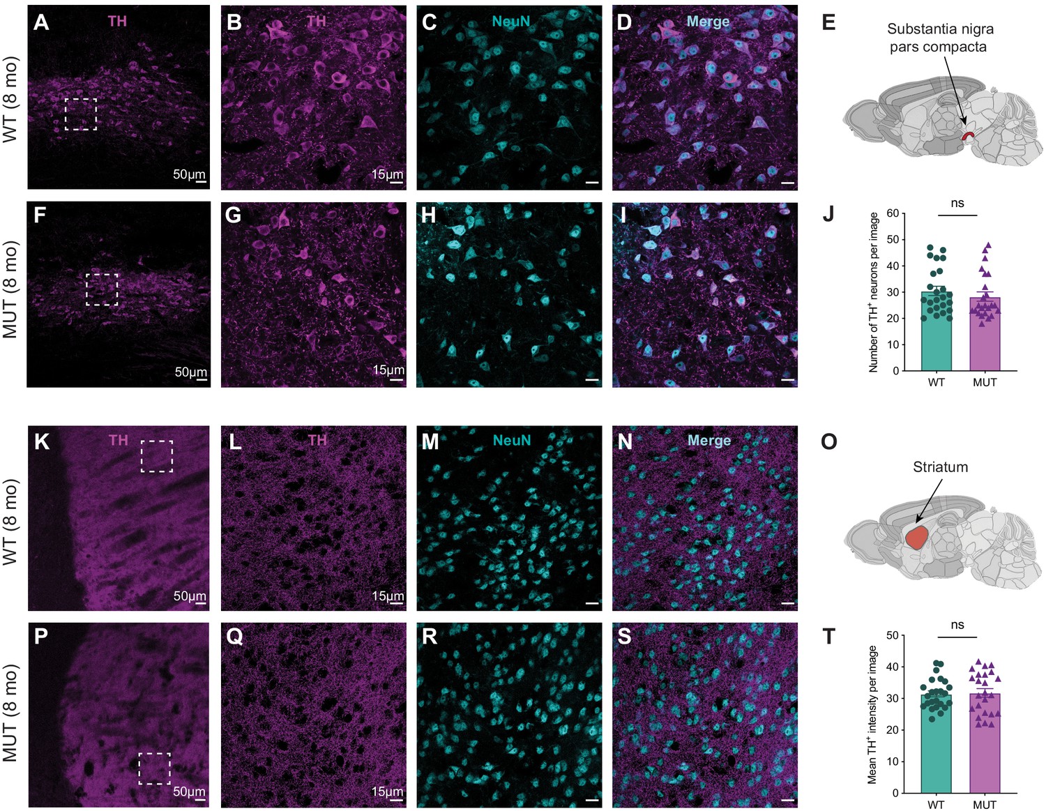
Dopaminergic innervation is not significantly different between aged WT and MUT mice.
(A) Representative 10x image of tyrosine hydroxylase (TH) staining in the substantia nigra pars compacta (SNpc) of an 8-month-old WT mouse. Scale bar is 50 µm. (B–D) Representative 40x image of WT SNpc, depicting tyrosine hydroxylase+ (TH+) dopaminergic cell bodies (B), NeuN+ neuronal marker (C), and their merged image (D). Scale bars are 15 µm. (E) Schematic representation of brain region analyzed, substantia nigra pars compacta, adapted from Allen Brain Atlas (Oh et al., 2014). (F) Representative 10x image of TH staining in the substantia nigra pars compacta (SNpc) of an 8-month-old MUT mouse. Scale bar is 50 µm. (G–I) Representative 40x image of MUT SNpc, depicting tyrosine hydroxylase+ (TH+) dopaminergic cell bodies (G), NeuN+ neuronal marker (H), and their merged image (I). Scale bars are 15 µm. (J) Graph depicting the mean number of TH+ neurons per 40x image reveals no difference between WT and MUT SNpc (8mo WT 30.5±1.78 cells, n=24 images, 8mo MUT 28.33 ± 1.77 cells, n=24 images; U=234, p=0.2695). (K) Representative 10x image of TH staining in the striatum of an 8-month-old WT mouse. Scale bar is 50 µm. (L–N) Representative 40x image of WT striatum depicting TH+ dopaminergic innervation (L), NeuN+ neuronal marker (M), and their merged image (N). Scale bars are 15 µm. (O) Schematic representation of brain region analyzed, striatum, adapted from Allen Brain Atlas (Oh et al., 2014). (P) Representative 10x image of TH staining in the striatum of an 8-month-old MUT mouse. Scale bar is 50 µm. (Q–S) Representative 40x image of MUT striatum depicting tyrosine hydroxylase+ (TH+) dopaminergic innervation (Q), NeuN+ neuronal marker (R), and their merged image (S). Scale bars are 15 µm. (T) Graph depicting the mean intensity of TH+ signal per 40x image reveals no significant difference between WT and MUT dopaminergic innervation (8mo WT 31.48 ± 0.97, n=24 images, 8mo MUT 31.80 ± 1.35, n=24 images; t41.82=0.1955, p=0.8459). Data obtained from three animals per condition and reported as mean ± standard error of the mean (SEM), with error bars as SEM. Mann–Whitney test (J) and two-tailed t-test (T).
Figure 7 with 2 supplements
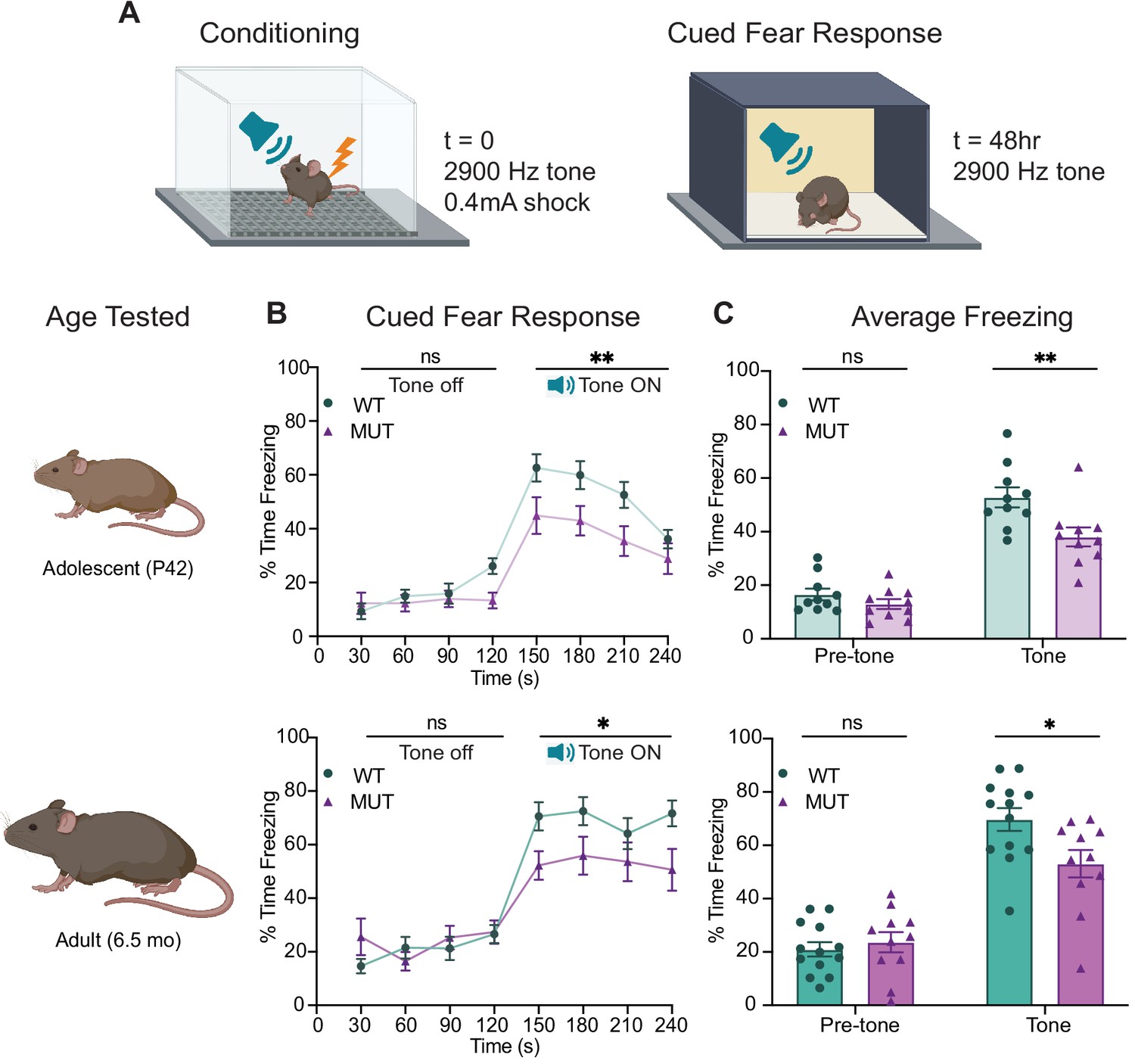
SWIPP1019R mutant mice display persistent deficits in cued fear memory recall.
(A) Experimental fear conditioning paradigm. After acclimation to a conditioning chamber, mice received a mild aversive 0.4mA footshock paired with a 2900 Hz tone. 48 hr later, the mice were placed in a chamber with different tactile and visual cues. The mice acclimated for two minutes and then the 2900 Hz tone was played (no footshock) and freezing behavior was assessed. (B) Line graphs of WT and MUT freezing response during cued tone memory recall. Data represented as average freezing per genotype in 30 s time bins. The tone is presented after t=120 s, and remains on for 120 s (Tone ON). Two different cohorts of mice were used for age groups P42 (top) and 6.5mo (bottom). Two-way ANOVA analysis of average freezing during Pre-Tone and Tone periods reveal a Genotype x Time effect at P42 (WT n=10, MUT n=10, F1,18=4.944, p=0.0392) and 6.5mo (WT n=13, MUT n=11, F1,22=13.61, p=0.0013). (C) Graphs showing the average %time freezing per animal before and during tone presentation. Top: freezing is reduced by 20% in MUT adolescent mice compared to WT littermates (Pre-tone WT 16.5 ± 2.2%, n=10; Pre-tone MUT 13.0 ± 1.8%, n=10; t36=0.8569, p=0.6366; Tone WT 52.8 ± 3.8%, n=10; Tone MUT 38.0 ± 3.6%, n=10; t36=3.539, p=0.0023), Bottom: freezing is reduced by over 30% in MUT adult mice compared to WT littermates (Pre-tone WT 21.1 ± 2.7%, n=13; Pre-tone MUT 23.7±3.8%, n=11; t44=0.4675, p=0.8721; Tone WT 69.7 ± 4.3%, n=13; Tone MUT 53.1 ± 5.2%, n=11; t44=2.921, p=0.0109). Data reported as mean ± SEM, error bars are SEM. *p<0.05, **p<0.01, two-way ANOVAs (B) and Sidak’s post hoc analyses (C).
Figure 7—figure supplement 1
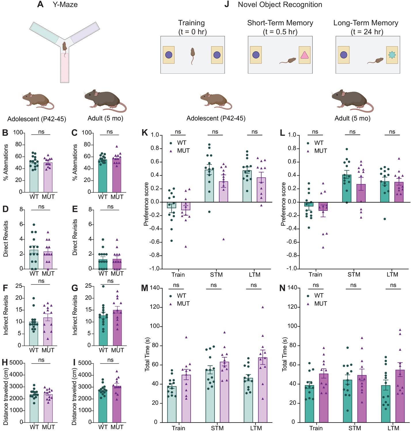
SWIPP1019R mutant mice do not display deficits in spatial working memory or novel object recognition.
(A) Y-maze paradigm. Mice were placed in the center of the maze and allowed to explore all three arms freely for five minutes. Each arm had distinct visual cues. (B) Graph depicting the percent alternations achieved for each mouse at adolescence (WT 51.48 ± 2.47%, MUT 50.81 ± 2.19%, t24=0.2036, p=0.8404). (C) Graph depicting the percent alternations achieved for each mouse at adulthood (WT 56.12 ± 1.53%, MUT 57.93 ± 2.56%, t18=0.6074, p=0.5511). (D) Graphs of the number of direct revisits mice made to the arm they just explored reveal no difference between genotypes at adolescence (WT 2.64 ± 0.50, MUT 2.42 ± 0.42, t24=0.3482, p=0.7308). (E) Graphs of the number of direct revisits mice made at adulthood (WT 1.36 ± 0.33, MUT 1.42 ± 0.36, t24=0.1231, p=0.9031). (F) Similar to D-E, there were no differences in the number of indirect revisits (ex: arm A→ arm B→arm A) between genotypes at adolescence (WT 10.21 ± 1.03, MUT 12.00 ± 1.48, U=69, p=0.4515). (G) Indirect revisits at adulthood (WT 12.86 ± 1.26, MUT 15.17 ± 1.43, t23=1.211, p=0.2380). (H) There were no significant differences in total distance traveled at adolescence, suggesting that motor function did not affect Y-maze performance (WT 2401 ± 98.9 cm, MUT 2406 ± 121.0 cm, t22=0.03281, p=0.9741). (I) No difference in distanced traveled at adulthood (WT 2761 ± 111.6 cm, MUT 3124 ± 191.1 cm, t18=1.638, p=0.1189). (J) Novel object task. Mice first performed a 5 min trial in which they were placed in an arena with two identical objects and allowed to explore freely, while their behavior was tracked with video software. Mice were returned to their home cage and then re-introduced to the arena a half an hour later, where one of the objects had been replaced with a novel object, and their behavior was again tracked. Twenty-four hours later the same test was performed, but the novel object was replaced with another new object. (K) Graph depicting adolescent animals’ preference for the novel object during the three phases of the task, training (Train), short-term memory (STM), and long-term memory (LTM). No significant difference in object preference is seen between genotypes for any phase (Train WT −0.092 ± 0.065, Train MUT −0.123 ± 0.072, STM WT 0.488 ± 0.076, STM MUT 0.315 ± 0.094, LTM WT 0.479 ± 0.046, LTM MUT 0.373 ± 0.076, F1,22=1.840, p=0.1887). (L) Graph depicting adult animals’ preference for the novel object. (Train WT −0.066 ± 0.053, Train MUT −0.130 ± 0.089, STM WT 0.416 ± 0.060, STM MUT 0.274 ± 0.096, LTM WT 0.316 ± 0.059, LTM MUT 0.306 ± 0.050, F1,22=0.9735, p=0.3345). (M) Graph depicting the total amount of time (in seconds) adolescent animals spent exploring both objects in each phase of the task. No significant difference in exploration time was observed across genotypes, suggesting that genotype does not hinder object exploration (Train P44 WT 38.10 ± 2.45 s, Train P44 MUT 50.04 ± 5.44 s, STM P44 WT 55.02 ± 4.31 s, STM P44 MUT 63.60 ± 4.50 s, LTM P45 WT 46.75 ± 3.34 s, LTM P45 MUT 68.08 ± 7.54 s, F1,22=7.373, p=0.0126). (N) Graph depicting the total time adult animals spent exploring both objects in each the task (Train WT 39.10 ± 3.62 s, Train MUT 51.15 ± 4.91 s, STM WT 44.75 ± 4.87 s, STM MUT 49.56 ± 6.16 s, LTM WT 39.02 ± 5.29 s, LTM MUT 55.15 ± 7.34 s, F1,22=2.936, p=0.1007). For all Y-maze measures, WT n=14, MUT n=12. For all novel object measures, WT n=13, MUT n=11. Data reported as mean ± SEM, error bars are SEM. Two-tailed t-tests or Mann–Whitney U tests (B–I), two-way ANOVAs (K–N).
Figure 7—figure supplement 2

SWIPP1019R mutant mice do not have significant deficits in contextual fear memory recall, auditory perception, or tactile sensation.
(A) Experimental fear conditioning scheme. After acclimation, mice received a mild aversive 0.4mA footshock paired with a 2900 Hz tone in a conditioning chamber. 24 hr later, the mice were placed back in the same chamber to assess freezing behavior (without footshock or tone). (B) Experimental startle response setup used to assess hearing and somatosensation. Mice were placed in a plexiglass tube atop a load cell that measured startle movements in response to stimuli. (C) Line graphs of WT and MUT freezing response during the contextual memory recall task. Data represented as average freezing per genotype in 30 s time bins. The task was performed with two different cohorts for the different ages, P42 (top) and 6.5mo (bottom). Top: no significant difference in freezing at P42 (Two-way repeated measure ANOVA, Genotype effect, F1,18=0.088, p=0.7698. Sidak’s post-hoc analysis, 30 s p=0.8388, 60 s p=0.9990, 90 s p=0.9964, 120 s p=0.3281), Bottom: no significant difference in freezing at 6.5mo (Two-way repeated measure ANOVA, Genotype effect, F1,22=3.723, p=0.0667. Sidak’s post-hoc analysis, 30 s p=0.8977, 60 s p=0.1636, 90 s p=0.9979, 120 s p=0.0037). (D) Graphs showing the average total freezing time per animal during context exposure. Top: no significant difference is seen between WT and MUT mice at P42 (WT 34.01 ± 6.32%, MUT 36.99 ± 7.81%, t17=2.985, p=0.7699). Bottom: no significant different is seen between genotypes at 6.5mo (WT 43.94 ± 6.00%, MUT 28.73 ± 4.80%, t21.6=1.980, p=0.0606). (E) Graphs of individual animals’ startle response to a 2900 Hz tone played at 80 dB. MUT mice were not significantly more reactive to the tone than WT at P50 (WT 25.96 ± 4.95, MUT 40.68 ± 5.05, U=35, p=0.2799), or at 6.5mo (WT 14.07 ± 3.27, MUT 14.85 ± 1.49, U=47, p=0.2768). (F) Graphs of individual animals’ startle response to a 0.4mA footshock. No significant difference observed between genotypes at either age (P55 WT 1527 ± 215.7, P55 MUT 1996 ± 51.0, U=28.50, p=0.0542; 6.5mo WT 1545 ± 179.5, 6.5mo MUT 1817 ± 119.1, U=47, p=0.2360). Startle response reported in arbitrary units (AU). For all adolescent measures: WT n=10, MUT n=10. For adult freezing measures: WT n=13, MUT n=11. For adult startle responses: WT n=13, MUT n=10. Data reported as mean ± SEM, error bars are SEM.*p<0.05, **p<0.01, two-way repeated measure ANOVAs (C), two-tailed t-tests (D), and Mann–Whitney U tests (E–F).
Figure 8 with 1 supplement
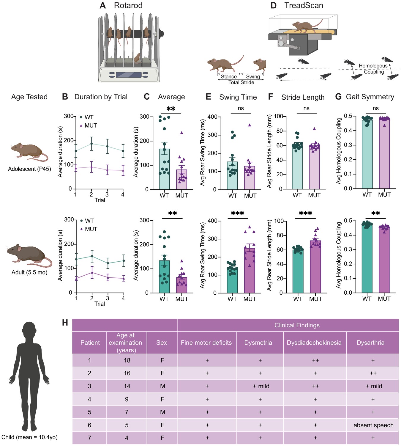
SWIPP1019R mutant mice exhibit surprising motor deficits that are confirmed in human patients.
(A) Rotarod experimental setup. Mice walked atop a rod rotating at 32 rpm for 5 min, and the duration of time they remained on the rod before falling was recorded. (B) Line graph of average duration animals remained on the rod per genotype across four trials, with an inter-trial interval of 40 min. The same cohort of animals was tested at two different ages, P45 (top) and 5.5 months (bottom). Genotype had a significant effect on task performance at both ages (top, P45: genotype effect, F1,25=7.821, p=0.0098. bottom, 5.5mo: genotype effect, F1,23=7.573, p=0.0114). (C) Graphs showing the average duration each animal remained on the rod across trials. At both ages, the MUT mice exhibited an almost 50% reduction in their ability to remain on the rod (top, P45: WT 169.9 ± 25.7 s, MUT 83.8 ± 15.9 s, U=35, p=0.0054; bottom, 5.5mo: WT 135.9 ± 20.9 s, MUT 66.7 ± 9.5 s, t18=3.011, p=0.0075). (D) TreadScan task. Mice walked on a treadmill for 20 s while their gate was captured with a high-speed camera. Diagrams of gait parameters measured in (E–G) are shown below the TreadScan apparatus. (E) Average swing time per stride for hindlimbs. At P45 (top), there is no significant difference in rear swing time (WT 156.2 ± 22.4 ms, MUT 132.3 ± 19.6 ms, U=83, p=0.7203). At 5.5mo (bottom), MUT mice display significantly longer rear swing time (WT 140 ± 6.2 ms, MUT 252.0 ± 21.6 ms, t12=4.988, p=0.0003). (F) Average stride length for hindlimbs. At P45 (top), there is no significant difference in stride length (WT 62.3 ± 2.0 mm, MUT 60.5 ± 2.1 mm, U=75, p=0.4583). At 5.5mo (bottom), MUT mice take significantly longer strides with their hindlimbs (WT 60.8 ± 0.8 mm, MUT 73.6 ± 2.7 mm, t11.7=4.547, p=0.0007). (G) Average homologous coupling for front and rear limbs. Homologous coupling is 0.5 when the left and right feet are completely out of phase. At P45 (top), WT and MUT mice exhibit normal homologous coupling (WT 0.48 ± 0.005, MUT 0.48 ± 0.004, U=76.5, p=0.4920). At 5.5 mo (bottom), MUT mice display decreased homologous coupling, suggestive of abnormal gait symmetry (WT 0.48 ± 0.003, MUT 0.46 ± 0.004, t18.8=3.715, p=0.0015). At P45: n=14 WT, n=13 MUT; At 5.5mo: n=14 WT, n=11 MUT. (H) Table of motor findings in clinical exam of human patients with the homozygous SWIPP1019R mutation. All patients exhibit motor dysfunction (+ = symptom present). Data reported as mean ± SEM, error bars are SEM. *p<0.05, **p<0.01, ***p<0.001, ****p<0.0001, two-way repeated measure ANOVAs (B), Mann–Whitney U tests and two-tailed t-tests (C–G).
Figure 8—figure supplement 1

Progressive gait changes in SWIPP1019R mutant mice are not restricted to rear limbs.
(A) Graph of average swing time per stride for front limbs. At P45 (top), there is no significant difference in front swing time (WT 177.5 ± 10.9 ms, MUT 175.3 ± 8.7 ms, t24=0.1569, p=0.8766). At 5.5 mo (bottom), MUT mice take significantly longer to swing their forelimbs (WT 178.6 ± 6.2 ms, MUT 206.3 ± 7.2 ms, t21.4=2.927, p=0.0079). (B) Graph of average stride length for front limbs. At P45 (top), there is no difference in WT and MUT stride length (WT 57.0 ± 0.9 mm, MUT 59.2 ± 1.4 mm, U=68, p=0.2800). At 5.5mo (bottom), MUT mice take significantly longer strides with their forelimbs (WT 60.0 ± 0.6 mm, MUT 63.7 ± 0.9 mm, t17=3.545, p=0.0024). (C) Graph of average homolateral coupling, the fraction of a reference foot’s stride when its ipsilateral foot starts its stride. At P45, there is no significant difference in homolateral coupling (WT 0.48 ± 0.005, MUT 0.48 ± 0.004, U=90, p=0.9713), but at 5.5mo, MUT mice display decreased homolateral coupling (WT 0.48 ± 0.002, MUT 0.45 ± 0.005, t13.5=3.469, p=0.0039). (D) Graph of average track width between front limbs. At P45 (top), there is a significantly narrower front track width in MUT compared to WT (WT 16.99 ± 0.15 mm, MUT 15.12 ± 0.33 mm, t17=5.192, p<0.0001). This difference persists into adulthood at 5.5mo (WT 19.36 ± 0.23 mm, MUT 16.74 ± 0.46 mm, t15=5.055, p=0.0001). (E) Graph of average track width between rear limbs. At P45 (top), there is no difference in WT and MUT rear track widths (WT 29.58 ± 0.51 mm, MUT 28.77 ± 0.36 mm, t23=1.292, p=0.2091). At 5.5mo (bottom), mutants display significantly narrower rear track widths (WT 32.59 ± 0.34 mm, MUT 30.01 ± 0.46 mm, t19.4=4.502, p=0.0002). For P45 measures: WT n=14, MUT n=13; for 5.5mo measures: WT n=14, MUT n=11. Data reported as mean ± SEM, error bars are SEM. **p<0.01, ***p<0.001, ****p<0.0001, two-tailed t-tests or Mann–Whitney U tests.
Figure 9
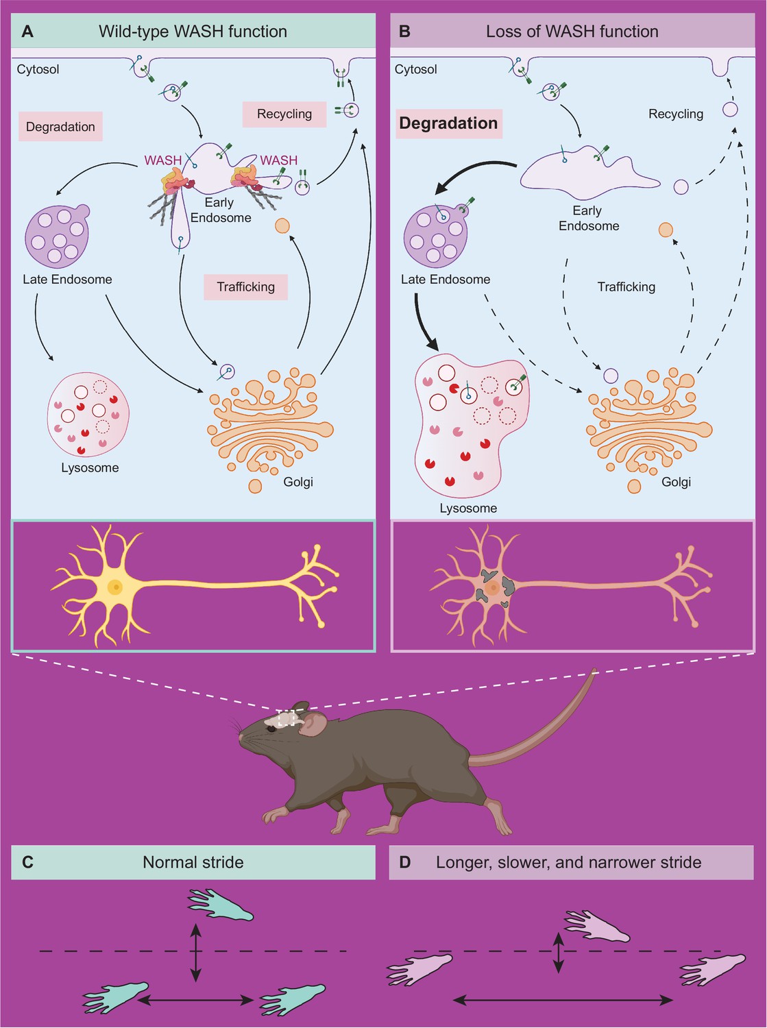
Model of neuronal endo-lysosomal pathology in SWIPP1019R mutant mice.
(A) Wild-type WASH function in mouse brain. Under normal conditions, the WASH complex interacts with many endosomal proteins and cytoskeletal regulators, such as the Arp2/3 complex. These interactions enable restructuring of the endosome surface (actin in gray) and allow for cargo segregation and scission of vesicles. Substrates are transported to the late endosome for lysosomal degradation, to the Golgi network for modification, or to the cell surface for recycling. (B) Loss of WASH function leads to increased lysosomal degradation in mouse brain. Destabilization of the WASH complex leads to enlarged endosomes and lysosomes, with increased substrate accumulation at the lysosome. This suggests an increase in flux through the endo-lysosomal pathway, possibly as a result of mis-localized endosomal substrates. (C) Wild-type mice exhibit normal motor function. (D) SWIPP1019R mutant mice display progressive motor dysfunction in association with these subcellular alterations.
Tables
Key resources table
| Reagent type (species) or resource | Designation | Source or reference | Identifiers | Additional information |
|---|---|---|---|---|
| Gene (Homo sapiens) | WASHC4 | GenBank | Gene ID: 23325 | Aka SWIP |
| Gene (Mus musculus) | Washc4 | Ensembl | ENSMUSG00000034560 | |
| Strain, strain background (Mus musculus) | SWIPP1019R | This paper, Duke Transgenic Mouse Facility | ENSMUSG00000034560 | Mouse line maintained by Soderling lab |
| Strain, strain background (Mus musculus) | B6SJLF1/J | Jackson Laboratories | Cat# 100012 RRID:IMSR_JAX:100012 | |
| Strain, strain background (Mus musculus) | C57BL/6J | Jackson Laboratories | Cat# 000664 RRID:IMSR_JAX:000664 | |
| Recombinant DNA reagent | pmCAG-SWIP-WT-HA (plasmid) | This paper | SWIP-WT | AAV construct to transfect and express the recombinant DNA Sequence |
| Recombinant DNA reagent | pmCAG-SWIP-MUT-HA (plasmid) | This paper | SWIP-MUT | AAV construct to transfect and express the recombinant DNA Sequence |
| Recombinant DNA reagent | phSyn1-WASH1-BioID2-HA (plasmid) | This paper | WASH1-BioID2 | Transduced AAV construct Sequence |
| Recombinant DNA reagent | phSyn1- solubleBioID2-HA (plasmid) | This paper | SolubleBioID2 control | Transduced AAV construct Sequence |
| Recombinant DNA reagent | pAd-DeltaF6 | Addgene | pAd-DeltaF6 | Helper plasmid for AAV2/9 viral preparation Sequence |
| Recombinant DNA reagent | pAAV2/9 | Addgene | pAAV2/9 | Viral capsid Sequence |
| Cell line (Mus musculus) | Primary mouse cortical cultures | This paper | SWIP WT, SWIPP1019RMUT neurons | Freshly isolated from wild-type or SWIPP1019R P0 mouse brains |
| Cell line (Homo sapiens) | Human Embryonic Kidney 293 T cells | Duke Cell Culture Facility | ATTC Cat# CRL-11268 RRID:CVCL_1926 | |
| Sequence-based reagent | Washc4 CRISPR sgRNA | This paper | Oligonucleotide sequence | N20+ PAM sequence targeting mouse Washc4 gene for introducing C/G mutation 5′ttgagaatactcacaagagg agg3′ |
| Sequence-based reagent | Washc4_F repair | This paper | Forward repair oligonucleotide | Forward strand of the repair oligo used to introduce C/G mutation into mouse Washc4 gene 5′atttcgaaggccaaagaatatacatctccgaaatttctatatcattgttcgtcctcttgtgagtattctcaaaactagaagtgagttattgatgggtgttaatacagattcagtttccataaagca3′ |
| Sequence-based reagent | Washc4_R repair | This paper | Reverse repair oligonucleotide | Reverse strand of the repair oligo used to introduce C/G mutation into mouse Washc4 gene 5′tgctttatggaaactgaatctgtattaacacccatcaataactcacttctagttttgagaatactcacaagaggacgaacaatgatatagaaatttcggagatgtatattctttggccttcgaaat3′ |
| Sequence-based reagent | Washc4_F mutagenesis | This paper | Forward primer | Washc4 C/G mutagenesis forward primer 5′ctacaaagttgagggtcagacggggaacaattatatagaaa3′ |
| Sequence-based reagent | Washc4_R mutagenesis | This paper | Reverse primer | Washc4 C/G mutagenesis reverse primer 5′tttctatataattgttccccgtctgaccctcaactttgtag3′ |
| Sequence-based reagent | Washc4_F genotyping | This paper | Forward primer | Washc4 forward primer for genotyping SWIPP1019R mice 5′tgcttgtagatgtttttcct3′ |
| Sequence-based reagent | Washc4_R genotyping | This paper | Reverse primer | Washc4 reverse primer for genotyping SWIPP1019R mice 5′gttaacatgatcctatggcg3′ |
| Antibody | Anti-human WASH1 (C-terminal, rabbit monoclonal) | Sigma Aldrich | Cat# SAB42200373 | WB (1:500) |
| Antibody | Anti-human Strumpellin (rabbit polyclonal) | Santa Cruz | Cat# sc-87442 RRID:AB_2234159 | WB (1:500) |
| Antibody | Anti-human EEA1 (rabbit monoclonal) | Cell Signaling Technology | Clone# C45B10 Cat# 3288 RRID:AB_2096811 | WB (1:1500) ICC (1:500) |
| Antibody | Anti-human LAMP1 (rabbit monoclonal) | Cell Signaling Technology | Clone# C54H11 Cat# 3243 RRID:AB_2134478 | WB (1:2000) |
| Antibody | Anti-human Beta Tubulin III (mouse monoclonal) | Sigma Aldrich | Clone# SDL.3D10 Cat# T8660 RRID:AB_477590 | WB (1:10,000) |
| Antibody | Anti-human HA (mouse monoclonal) | BioLegend | Clone# 16B12 Cat# MMS-101P RRID:AB_10064068 | WB (1:5000) |
| Antibody | Anti-mouse Cathepsin D (rat monoclonal) | Novus Biologicals | Clone# 204712 Cat# MAB1029 RRID:AB_2292411 | ICC (1:250) |
| Antibody | Anti-human MAP2 (guinea pig polyclonal) | Synaptic Systems | Cat# 188004 RRID:AB_2138181 | ICC (1:500) |
| Antibody | Anti-human Cleaved Caspase-3 (rabbit polyclonal) | Cell Signaling Technology | Specificity Asp175 Cat#9661 RRID:AB_2341188 | IHC (1:2000) |
| Antibody | Anti-human Calbindin (mouse monoclonal) | Sigma Aldrich | Clone# CB-955 Cat# C9848 RRID:AB_476894 | IHC (1:2000) |
| Antibody | Anti-human HA (rat monoclonal) | Sigma Aldrich | Clone# 3F10 Cat# 11867423001 RRID:AB_390918 | IHC (1:500) |
| Antibody | Anti-human Bassoon (mouse monoclonal) | Abcam | Clone# SAP7F407 Cat# ab82958 RRID:AB_1860018 | IHC (1:500) |
| Antibody | Anti-human Homer1 (rabbit polyclonal) | Synaptic Systems | Cat# 160002 RRID:AB_2120990 | IHC (1:500) |
| Antibody | Anti-human Tyrosine Hydroxylase (chicken polyclonal) | Abcam | Cat# ab76442 RRID:AB_1524535 | IHC (1:1000) |
| Antibody | Anti-human NeuN (mouse monoclonal) | Abcam | Clone# 1B7 Cat# ab104224 RRID:AB_10711040 | IHC (1:1000) |
| Commercial assay or kit | TMTpro 16plex Label Reagent | Thermo Fisher | Cat# A44520 | |
| Commercial assay or kit | NeutrAvidin Agarose Resins | Thermo Fisher | Cat# 29201 | |
| Commercial assay or kit | S-Trap Binding Buffer | Profiti | Cat# K02-micro-10 | |
| Commercial assay or kit | QuikChange XL Site-Directed Mutagenesis Kit | Agilent | Cat# 200517 | |
| Software, algorithm | Courtland et al., source code | GitHub | ||
| Software, algorithm | MSstatsTMT | GitHub | PubMed | |
| Software, algorithm | leidenalg Python Library | conda | Version 0.8.1 | |
| Software, algorithm | Cytoscape | https://cytoscape.org/ | RRID:SCR_003032 | Version 3.7.2 |
| Software, algorithm | Imaris | Oxford Instruments | RRID:SCR_007370 | Version 9.2.0 |
| Software, algorithm | Zen | Zeiss | RRID:SCR_018163 | Version 2.3 |
| Software, algorithm | Fiji | https://fiji.sc/ | RRID:SCR_002285 | Version 2.0.0-rc-69/1.52 p |
| Software, algorithm | GraphPad Prism | GraphPad Software | RRID:SCR_002798 | Version 8.0 |
| Software, algorithm | Proteome Discoverer | Thermo Fisher | RRID:SCR_014477 | Versions 2.2 and 2.4 |
| Software, algorithm | TreadScan NeurodegenScanSuite | CleverSysInc | ||
| Software, algorithm | EthoVision XT | Noldus Information Technology | RRID:SCR_000441 | Version 11.0 |
| Software, algorithm | Rotarod apparatus for mouse | Med Associates | Cat# ENV-575M | |
| Software, algorithm | Fear conditioning chamber | Med Associates | Cat# VFC-008-LP | |
| Software, algorithm | FreezeScan software | CleverSysInc | RRID:SCR_014495 | |
| Software, algorithm | Startle reflex chamber and software | Med Associates | Cat# MED-ASR-PRO1 | |
| Other | Geladaki et al.’s, LOPIT-DC protocol | PubMed | PMCID:PMC6338729 | Subcellular fractionation protocol |
| Other | Orbitrap Fusion Lumos Tribrid Mass Spectrometer | Duke Proteomics and Metabolomics Shared Resource | Mass spectrometer used for spatial proteomics | |
| Other | Thermo QExactive HF-X Mass Spectrometer | Duke Proteomics and Metabolomics Shared Resource | Mass spectrometer used for iBioID | |
| Other | Zeiss 710 LSM confocal microscope | Duke Light Microscopy Core Facility (LCMF) | RRID:SCR_018063 | Confocal microscope used for image acquisition of ICC and IHC samples |
| Other | Reichert Ultracut E Microtome | Duke Department of Pathology | Microtome used to prepare TEM samples | |
| Other | Phillips CM12 Electron Microscope | Duke Department of Pathology | Transmission electron microscope used for TEM image acquisition | |
| Other | Beckman XL-90 Centrifuge and Ti-70 rotor | Duke Department of Cell Biology | Ultracentrifuge used for AAV virus preparation | |
| Other | Beckman TLA-100 Ultracentrifuge and TLA-55 rotor | Duke Department of Cell Biology | Ultracentrifuge used for spatial proteomics sample preparation | |
| Other | DAPI stain | Thermo Fisher | Cat# D1306 RRID:AB_2629482 | (1 µg/mL) |
Additional files
-
Supplementary file 1
WASH iBioID statistical results.
Raw data and statistical analyses for the in vivo BioID (iBioID) experiment (Figure 1). Normalized protein data were fit with a linear model to derive a model-based statistical comparison of WASH1-iBioID and solubleBioID2 control groups (Huang et al., 2020). 175 proteins were considered enriched in the WASH interactome by exhibiting a fold-change greater than four over the negative control with a Benjamini–Hochberg false discovery rate (FDR) less than 0.05 (Benjamini and Hochberg, 1995).
- https://cdn.elifesciences.org/articles/61590/elife-61590-supp1-v1.xlsx
-
Supplementary file 2
SWIPP1019R TMT protein-level statistical results.
Raw data and protein-level statistical analyses for the spatial proteomics TMT experiment (Figure 3). MSstatsTMT was used to assess two types of contrasts: intra-BioFraction comparisons between Mutant and Control conditions, and overall ‘Mutant-Control’ comparisons.
- https://cdn.elifesciences.org/articles/61590/elife-61590-supp2-v1.xlsx
-
Supplementary file 3
Module-level results from network analysis of SWIPP1019R proteomics.
Module membership and module-level statistical analyses for the spatial proteomics TMT experiment (Figure 3). Each module was fit with a linear mixed model. Contrasts between Mutant and Control groups were assessed to determine which modules had significantly altered levels between genotypes.
- https://cdn.elifesciences.org/articles/61590/elife-61590-supp3-v1.xlsx
-
Supplementary file 4
Module-level gene set enrichments of SWIPP1019R proteomics.
Gene set enrichment statistics for the identified modules (Figure 3, Supplementary file 3). Biological pathway information, including source pathway membership, is provided.
- https://cdn.elifesciences.org/articles/61590/elife-61590-supp4-v1.xlsx
-
Supplementary file 5
Plasmid constructs.
Description of plasmids used with corresponding DNA sequence files.
- https://cdn.elifesciences.org/articles/61590/elife-61590-supp5-v1.xlsx
-
Transparent reporting form
- https://cdn.elifesciences.org/articles/61590/elife-61590-transrepform-v1.pdf
Download links
A two-part list of links to download the article, or parts of the article, in various formats.
Downloads (link to download the article as PDF)
Open citations (links to open the citations from this article in various online reference manager services)
Cite this article (links to download the citations from this article in formats compatible with various reference manager tools)
Genetic disruption of WASHC4 drives endo-lysosomal dysfunction and cognitive-movement impairments in mice and humans
eLife 10:e61590.
https://doi.org/10.7554/eLife.61590


