A computational account of why more valuable goals seem to require more effortful actions
- Motivation, Brain and Behavior lab, Paris Brain Institute (ICM); Sorbonne Université; Inserm U1127; CNRS U7225, France
Figures
Figure 1

Experiment 1 design.
Top row: example trial. Each trial includes three phases: (1) display of the running route animation and the associated incentive, (2) choice between this high-effort high-gain (HEHG) option or an implicit (not displayed) low-effort 0-gain (LE0G) option, and (3) rating of anticipated energetic cost (AEC). Middle row: structure of a session. Each session includes a training phase, three blocks of 18 trials, a recalibration of AEC rating, and three additional blocks. The training phase comprised a practice session (running various routes on the treadmill) and a calibration session (learning to provide accurate energetic cost rating based on objective feedback). The recalibration session only included a series of ratings with objective feedback about the real energetic cost. Bottom row: Random draw performed at the end of each block among its 18 just-completed trials. Choice made by the participant during the randomly selected trial is reminded and then executed: if the participant accepted the high-effort offer, she must get onto the treadmill and complete the effortful running route, after which the associated reward is added to her total earnings. If she declined the high-effort offer, she must complete a default low-effort running route, and her total earnings remain unchanged.
Figure 2
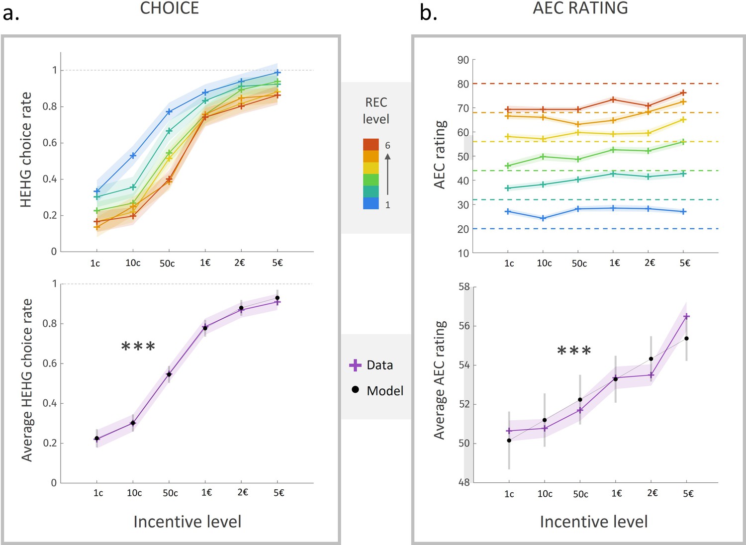
Choice rate and energetic cost rating in experiment 1.
(a) Rate of acceptance of the high-effort high-gain (HEHG) offer, plotted against incentive level. Top: cross markers indicate acceptance rate averaged across all participants for a given incentive level (x-axis) and a given real energetic cost (REC) level (marker colour). Bottom: purple cross markers indicate acceptance rate, averaged across all REC levels and across all participants for a given incentive level. Black dots indicate averaged predictions of a logistic regression model (see main text). *** Positive effect of incentive level on acceptance rate, p<0.001. (b) Anticipated energetic cost (AEC) rating, plotted against incentive level. Top: cross markers indicate AEC ratings averaged across all participants for a given incentive level (x-axis) and a given REC level (marker colour). Dotted lines indicate the target rating for each REC level. Bottom: purple cross markers indicate AEC rating, averaged across all REC levels and across all participants for a given incentive level. Black dots indicate averaged predictions of a generalized linear model (GLM, see main text). ***Positive effect of incentive level on AEC rating, p<0.001. Solid lines represent a linear interpolation between averaged data points (or model predictions) for illustrative purposes only. Shaded area around curves or error bars across dots represent the standard error to the mean (s.e.m), computed across participants.
Figure 3
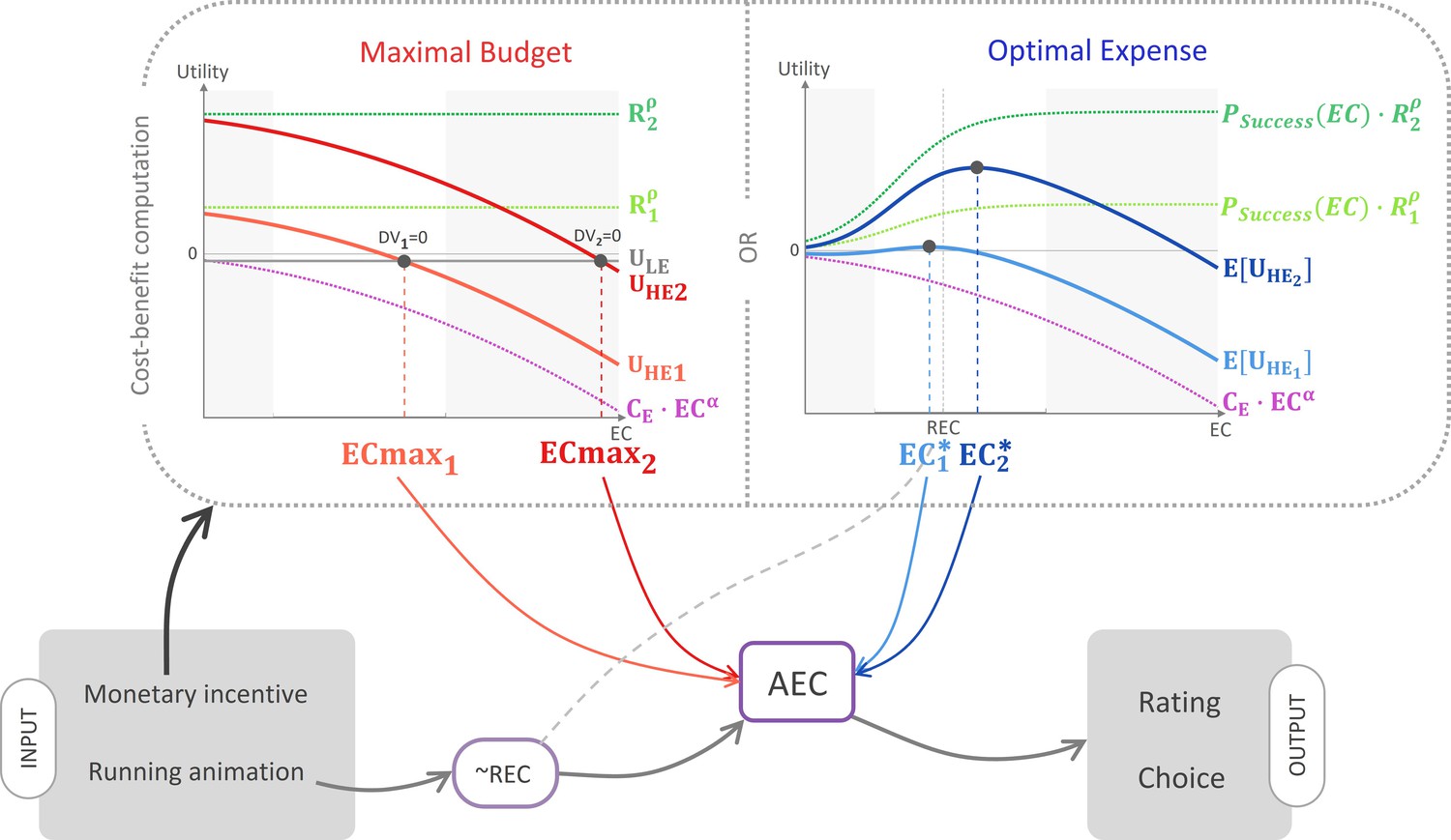
Schematic illustration of the ‘cost–benefit’ scenarios.
According to this hypothetical mechanism, information about the monetary incentive attached to the high-effort (HE) option enters a cost–benefit computation. According to the maximal budget variant (left panel), participants compute the maximal energetic cost above which the low-effort (LE) option would bear a higher utility (see Equations 1–3 in main text). According to the optimal expense variant, they compute the energetic cost optimizing the expected utility attached to the HE option (see Equations 7–9 in main text). In both panels, the computation is illustrated for two different reward magnitudes, R1 (small, light colour) and R2 (large, dark colour). Light grey areas correspond to domains outside the energetic cost rating scale. Both variants predict that larger incentives would result in a higher anticipated energetic cost (AEC) computation (see Equations 4 and 10), which also integrates a pre-estimate that is exclusively based on the running animation depicting the multi-segment route, and is thus a noisy reflection of the real energetic cost (REC). Finally, the resulting AEC estimate affects both energetic cost rating and choice between the HE offer and the LE reference option (see Equations 5 and 6 and Equations 11 and 12).
Figure 4
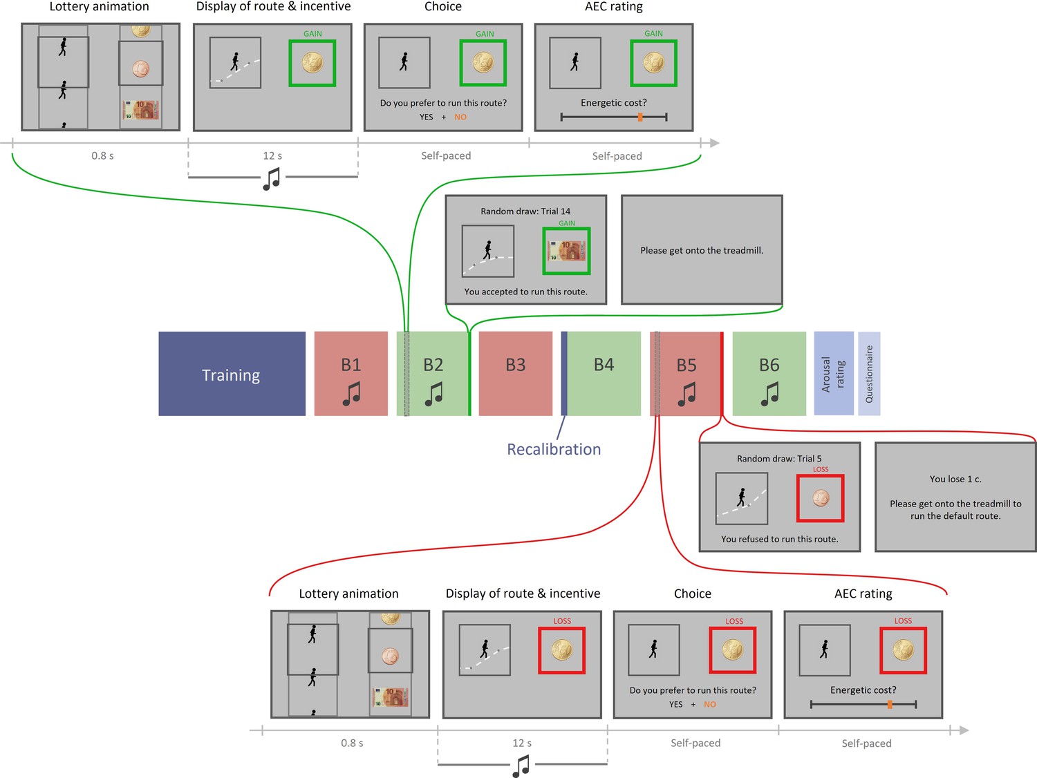
Experiment 2 design.
Top part, top row: example trial in the gain condition with music. Each trial includes four phases: (1) lottery animation, during which a running route and an incentive level are independently and (seemingly) randomly selected; (2) display of the running route animation and the associated incentive (potential gain here) while a musical extract plays in participant’s headset; (3) choice between this high-effort high-gain (HEHG) offer and an implicit low-effort 0-gain (LE0G) option; and (4) rating of anticipated energetic cost (AEC). Top part, bottom row: random draw performed at the end of a gain block among its 18 just-completed trials. Choice made by the participant is reminded then executed: in the gain condition, if the participant accepted the HEHG offer, she must get onto the treadmill and complete the effortful running route, after which the associated gain is added to her total earnings. If she declined the high-effort offer, she must complete a default low-effort running route, and her total earnings remain unchanged. Middle part: structure of a session. Each session includes a training phase (with practice on the treadmill and calibration of energetic cost rating with objective feedback), three blocks of 18 task trials, a recalibration (AEC ratings followed by objective feedbacks), three additional task trial blocks, a rating of arousal induced by all 72 musical extracts, and eventually a question about their belief in a general effort–reward correlation. Here, gain and loss conditions are alternated across blocks (green and red, respectively), and all blocks except B3 and B4 include musical extracts during display of route and incentive. Bottom part, bottom row: example trial in the loss condition with music. It is equivalent to the gain condition shown in top part, except that participants choose between a high-effort 0-loss (HE0L) and a low-effort high-loss condition (LEHL). Bottom part, top row: random draw performed at the end of a loss block among its 18 just-completed trials. Choice made by the participant is reminded then executed: in the loss condition, if the participant accepted the HE0L offer, she must get onto the treadmill and complete the effortful running route, and her total earnings remain unchanged. If she declined the high-effort offer, she must complete a default low-effort running route, after which the associated loss is subtracted from her total earnings.
Figure 5
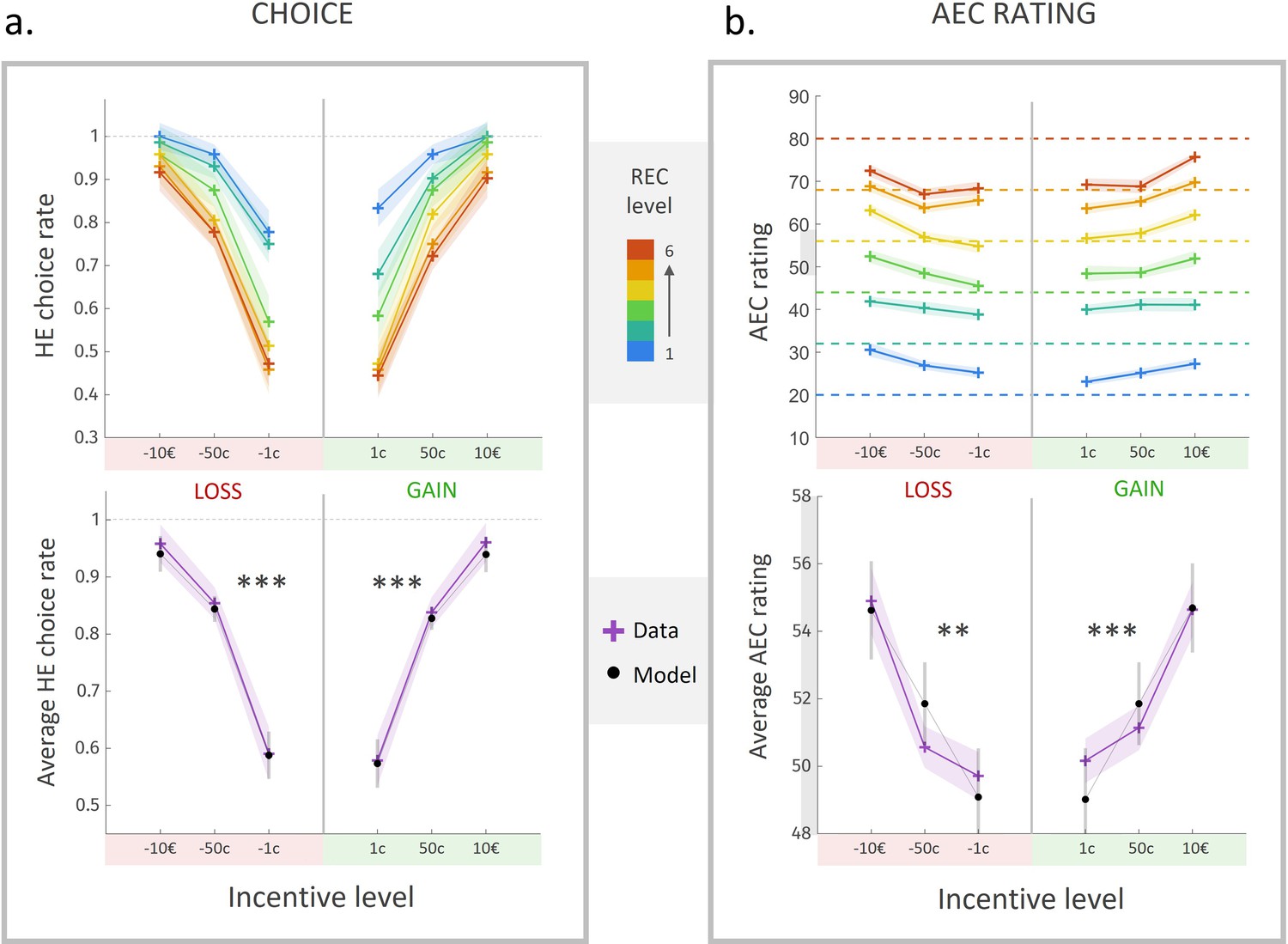
Choice rate and effort cost rating in experiment 2.
(a) Rate of acceptance of the high-effort offer, plotted against incentive level. Top: cross markers indicate acceptance rates averaged across all participants for a given incentive level (x-axis) and a given real energetic cost (REC) level (marker colour). Bottom: cross markers indicate acceptance rate, averaged across all REC levels and across all participants for a given incentive level. Black dots indicate averaged predictions of a logistic regression model (see main text). ***Positive effect of loss and gain level on acceptance rate, both p<0.001. (b) Anticipated energetic cost (AEC) rating, plotted against incentive level. Top: cross markers indicate AEC ratings averaged across all participants for a given incentive level (x-axis) and a given REC level (marker colour). Dotted lines indicate the target rating for each REC level. Bottom: cross markers indicate AEC ratings, averaged across all REC levels and across all participants for a given incentive level. Black dots indicate averaged predictions of a generalized linear model (GLM, see main text). **Positive effect of loss level on AEC rating, p<0.005. ***Positive effect of gain level on AEC rating, p<0.001. Solid lines represent a linear interpolation between averaged data points for illustrative purposes only. Shaded area around each curve represents the standard error to the mean (s.e.m), computed across participants.
Figure 6
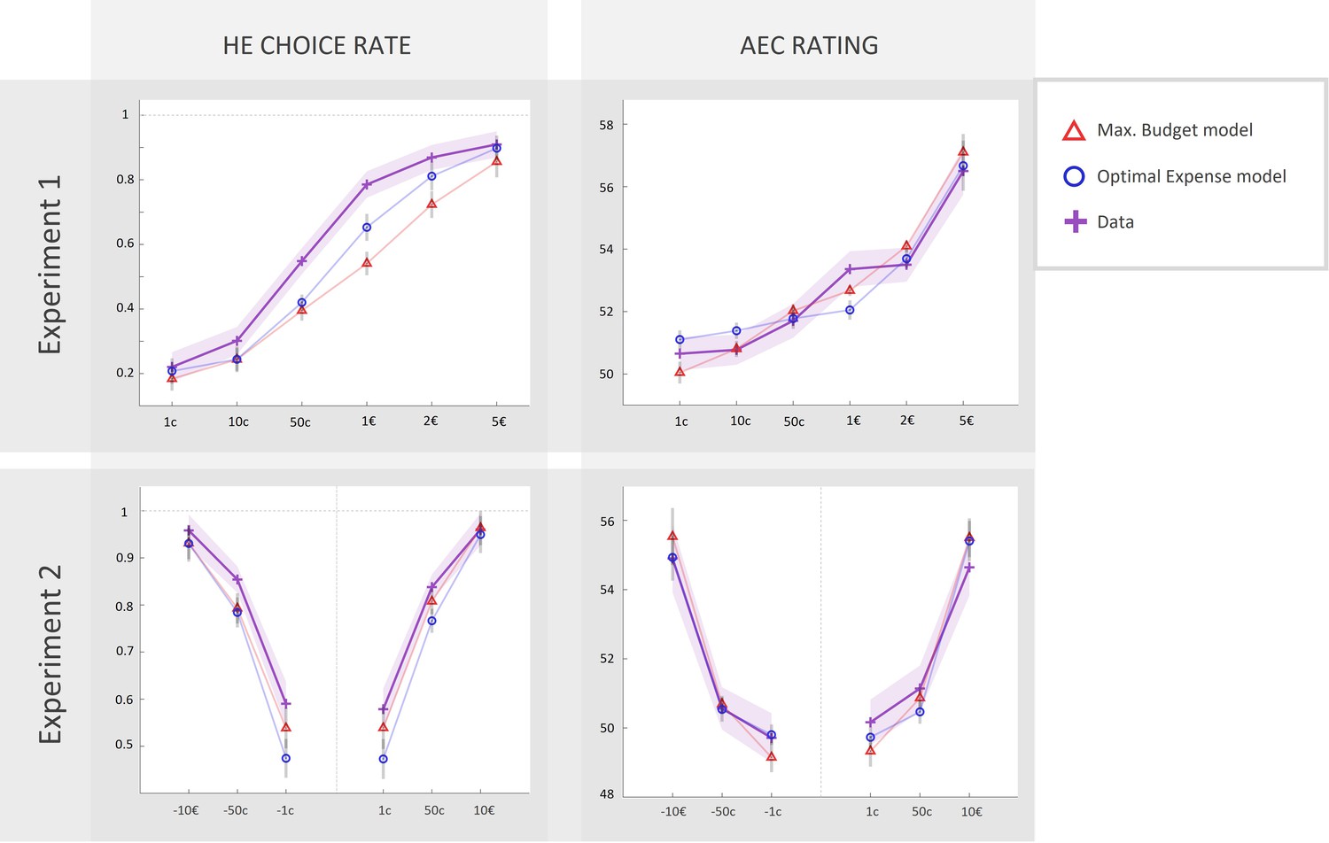
Fits of computational models to observed data in experiments 1 and 2 (N = 46).
Left column: rate of acceptance of the high-effort offer, plotted against incentive levels. Right column: anticipated effort cost (AEC) rating, plotted against incentive level. Cross markers indicate observed responses averaged across all real energetic cost (REC) levels and across all participants in experiment 1 or 2 (top or bottom line, respectively) for a given incentive level. Triangles and circles indicate averaged responses generated by the ‘maximal budget’ and ‘optimal expense’ models, respectively, with parameters fitted to individual data (both ratings and choices in both experiments). Solid lines represent a linear interpolation between averaged observed or modelled responses for illustrative purposes only. Shaded area around each line represents the standard error to the mean (s.e.m), computed across participants.
Figure 7
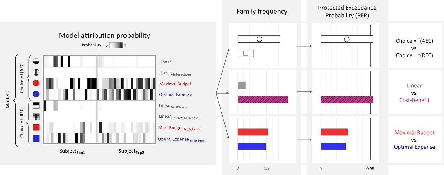
Bayesian model comparison across experiments 1 and 2 (N = 46).
Left: model attribution probability for each participant in experiments 1 and 2 (x-axis) and each model variant (y-axis). First four models from top correspond to the ‘standard’ variant, wherein the probability of choosing the high-effort option depends on the anticipated effort cost (AEC), while last four models correspond to the ‘null choice’ variant, wherein this probability depends on the real energetic cost (REC). Right: estimated frequency and protected exceedance probability (PEP) of each model family. PEP is the probability that a given model family is more frequent than any other one in the population, corrected for chance fluctuations of observed individual model evidences. Here, , and .
Appendix 1—figure 1
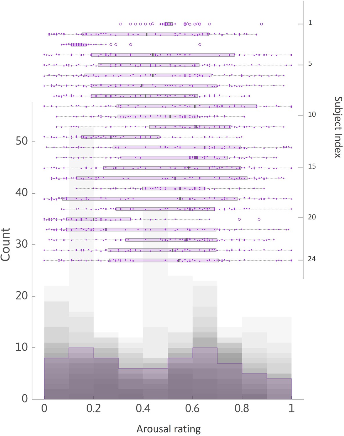
Distribution of arousal ratings in experiment 2.
Histogram plot, left y-axis: distributions of arousal ratings made about 72 musical extracts (ratings normalized to [0; 1]) overlaid across all subjects. Grey shade indicates the number of subjects who reached a given count (or above) for each given rating bin. Purple area delineates the group-averaged distribution. Whisker plots, right y-axis: all ratings and summary statistics of each subject. Each dot represents a rating, main vertical grey bar is the median, left and right ends of boxplot are first and third quartile of the distribution, respectively.
Appendix 1—figure 2

Pupil diameter during arousal rating task in experiment 2.
Pupil diameter as a function of elapsed time since the onset of each musical extract. Time courses were median-split between trials in which a high versus low arousal rating was given. Solid lines represent time courses averaged across corresponding trials and all experiment 2 subjects. Shaded area around each curve represents the standard error to the mean (s.e.m), computed across subjects. Vertical grey area highlights the time window during which pupil diameter was larger for high-arousal extracts (time window: [1.67–2.55] s post music onset, corrected for multiple comparisons). Left and right vertical dotted lines indicate music onset and rating onset, respectively.
Author response image 1
Author response image 2

Additional files
Download links
A two-part list of links to download the article, or parts of the article, in various formats.
Downloads (link to download the article as PDF)
Open citations (links to open the citations from this article in various online reference manager services)
Cite this article (links to download the citations from this article in formats compatible with various reference manager tools)
A computational account of why more valuable goals seem to require more effortful actions
eLife 11:e61712.
https://doi.org/10.7554/eLife.61712


